Using Principal Component Analysis and Least Squares Support Vector Machine to Predict the Silicon Content in Blast Furnace System

Using Principal Component Analysis and

Least Squares Support Vector Machine to Predict the

Silicon Content in Blast Furnace System

https://doi.org/10.3991/ijoe.v14i04.8397

Shihua Luo, Tianxin Chen!!_"

Jiangxi University of Finance & Economics, Nanchang, China [email protected]

Ling Jian

China University of Petroleum, Qingdao, China

Abstract—Blast furnace system is a typical example of complex industrial system. The silicon ([Si]) content in blast furnace system is an important index to reflect the temperature of furnace. Therefore, it is significant to carry out an accurate predictive control of furnace temperature. In this paper a composite model combining Principal Component Analysis (PCA) and Least Squares Support Vector Machine (LSSVM) is established to predict the furnace temper-ature. At the very beginning, in order to avoid redundancy and excessive noise pollution, PCA method is applied to reduce the dimensionality of original input variables. Secondly, the dimension-reduced variables are introduced to predict the silicon content by applying the LSSVM model. Finally, the result is com-pared with direct multivariable LSSVM prediction. The simulation results show that the new algorithm has positive significance as it achieves more obvious prediction hit rate (more than 80%) than direct multivariable LSSVM (with rate lower than 75%)..

Keywords—blast furnace system; principal component analysis; least squares support vector machine; silicon content prediction

1

Introduction

hearth, so it is usually used as the main index of smelting process control. The predic-tion and control of blast furnace temperature ([Si]) has always been a hot and difficult problem in this field[1-2].

The accurate prediction of furnace temperature and the linkage relationship be-tween furnace temperature, coal injection, air volume, air temperature and coke load are the key and difficult points in the modeling of blast furnace smelting process. Since entering the new century, due to truly understand the internal dynamics of phys-ical and chemphys-ical reactions in blast furnace is very difficult. The model research based on the mechanism of temperature prediction has gradually stagnated. What’s more,, the research on Intelligent Furnace Temperature Prediction Control based on intelligent algorithm is developing rapidly. Many domestic and foreign research teams have established many models such as Bayesian network model[3], chaotic prediction model[4], neural network model based on genetic algorithm[5], fuzzy data generation rule control model[6-7], partial least squares model[8], mathematical model of mul-tifluid theory[9], support vector machine and intelligent algorithm cross model[10], wavelet analysis model etc. These models obtain satisfactory results in different as-pects; however, due to the complexity of the blast furnace system, it is difficult to achieve closed-loop predictive control in this field.

Analyzing the existing prediction model, we found that some models only used single silicon content of ([Si]) sequences without many key state and control varia-bles, this is not reality. Some multivariable models have too many variavaria-bles, which lead to the shortage such as: modeling variables, information redundancy, noise pollu-tion and computapollu-tional complexity. It also restricts the practical applicapollu-tion of the model. Based on this, this paper concludes the advantages and disadvantages of prin-cipal component analysis (PCA) [11-15] and least squares support vector machine (LSSVM) [15-25] model, and constructs a new multivariable combination forecasting model for furnace temperature prediction.

In order to rationalize the multivariate information modeling, we use PCA method to take a plurality of variables influencing the silicon content integration become the main variable which is a linear combination of the initial variables. On the one hand, the number of input variables can be reduced and the model dimension reduction can be realized. Using this model, the number of input variables can be reduced and the model dimension reduction can be realized, on the other hand, information redundan-cy and noise pollution can be avoided, and the computational complexity can be sig-nificantly reduced. Then the LSSVM algorithm is used to predict the silicon content by introducing these composite variables. The simulation results show that the predic-tion algorithm based on PCA and LSSVM is better than LSSVM's direct multivariate modeling prediction.

2

Basic methods

2.1 Principal component analysis (PCA)

PCA is a commonly used dimension reduction method. Consider T

p

x

x

x

X

=

(

1

,

2

,

!

)

, X stands for a random vector of p dimensions, the covariance matrix can be written as:

p p pp p p p p X ! " " " " " # $ % % % % % & ' =

(

) ) ) ) ) ) ) ) ) … ! " ! ! # # 2 1 2 22 21 1 12 11 (1) p

!

!

!

1, 2,! are the p nonzero eigenvalues of the covariance matrices. Generally speaking,

!

1>

!

2 >…>

!

_p, according to the knowledge of linear algebra, there must be an orthogonal matrix

U

_,

U

satisfies the following equations:

p p p X T _U U ! " " " " " # $ % % % % % & ' =

(

) ) ) ! 2 1 (2) Among them, U is exactly the orthogonal matrix of the p eigenvectors correspond-ing to the p characteristic roots of the covariance matrix, U can be rewritten as:

11 12 1

21 22 2

1 2

p

p

p p _{pp p p}

U U U

U U U

U

U U U _!

" # $ % $ % = $ % $ % $ % & ' ! ! " " # "

$ ₍₃₎

1 2

( , , )T

i i i pi

U = U U ! U , T

m

Y Y Y

Y=( 1, 2,! ) as a principal component vector,

m

Y

Y

Y

1

,

2

,

!

can be regarded as the m principal component(m<p).Then

Y

can be expressed asY ₌UTX_{.Furthermore, the new principal component variables can be}

illustrated linearly by the original variables, which can be described as:

1 11 1 21 2 1

2 12 1 22 2 2

1 1 2 2

; ;

p p

p p

m m m pm p

Y U X U X U X

Y U X U X U X

Y U X U X U X

= + +

!

" _{= + +} "

# "

" _{= + +} $

! ! "

! ₍₄₎

(1)

Y

i

,

Y

j

i

!

j

;

i

,

j

=

,1

2

,

!

m

)

should be mutual independence, which means that

)

(,

0

)

,

cov(

Y

i

Y

j

=

i

!

j

;

(2)

Y

1

,

Y

2

,

!

Y

_{m should satisfy the diminishing of variance, which meant to be}

) ( )

( )

(Y₁ VarY₂ VarYm

Var > >! . It reflects the amount of information contained in the principal component variable is gradually reduced.

As demonstrated above, the variance of principal components are equal to their re-spective eigenvalues. It is obvious that

Var

(

Y

_k

)

=

!

_{k (}k =_1,2,!m₎. In addition, the

variance contribution rate of the principal component can be depicted as:

)

,

2

,

1

(

1

m

k

m

k k

k

k

=

=

!

!

=

"

"

#

(5)

If

!

_kis increasing, the variance contribution rate of the principal component

Y

_kis greater than the other principal components therefore

Y

_kintegratesX information better. Otherwise,

Y

₁

,

Y

₂

,

!

Y

_m, their ability to integrateXinformation is progressive-ly decreasing. In order to choose component m(m<p)!the cumulative contribution rate can be applied. Consider

1

1

m i i

p i i !

!

=

=

"

"

as the cumulative contribution rate of m

prin-cipal components!popularly, we assume that the value of m makes the cumulative contribution rate greater than 85%, and the effect is better. The m principal compo-nent can contain the information of most of the p variablesX . Thus, we use PCA to eliminate the noise of original variable dimension most of which not only can keep the original variable information, but also can reduce the number of variables, the sample properties and the amount of computation.

2.2 Least squares support vector machine (LSSVM)

The LSSVM uses kernel function to map the low dimensional linear non-separable samples into the high-dimensional space, so that the samples are linearly separable and can be predicted more accurately. Assume the training data set is

{

(

x

,

y

i

,1

2

,

n

)

}

T

=

i i

=

!

, where n is the number of training concentrated samples. n

i

R

x

!

is the input variables while

y

_i

!

R

nis the output variables. Under linear con-ditions, we construct the optimal decision function:

b

x

y

=

!

T

+

)

,

,

(

!

1

!

2

!

n

!

=

!

is an unknown parameter vector which can be considered as

the weight of all samples, b!R is the critical value. When input variables are nonlin-ear, we need to build a map

!

,

!

:

R

n

"

R

n! _{expressed by kernel function which is} able to linearization X by lifting the its dimension. In high-dimensional space, the optimal decision function can be expressed as:

b

x

y

=

#

!

"

(

)

+

(7)

which means

"

(

!

)

can use kernel function to calculate, such that

k

(

x

,

z

)

=

!

(

x

)

"

!

(

z

)

, as the kernel functions of variablesX andZ_{in high dimensional spaces, where}

n

R z

x, ! , a commonly used kernel function is the Radial Basis Function (RBF) kernel given by

!" ! # $

!% ! & ' (

=exp ,₂

) , (

) j i j

i

x x x

x k

(8)

!

is the usual Euclid norm and

!

is hyper parameter which can respond to the non-linear mapping

"

(!). In fact, the optimal decision function problem can be transformed

into a dual form. In order to solve

!

and b in the equation, the following two con-straints can be used to optimize the problem, which can be depicted as:

!

=

+

= N

i i T

b J ₁

2 ,

, 2 2

1 ) , (

min $ " $ $ # "

" $

(9)

The constraint condition is

y

_i

=

! "

$

( )

x

_i

+ +

b

#

_i,

!

is the penalty factor which represents the degree of penalty beyond the error sample and belongs to the adjustable parameter. In fact,

!

>

₀

, the smaller the

!

, the better sample that indicates the wrong fit;

!

_iis the loss function. For the sake of transform the constrained optimization prob-lem into an unconstrained probprob-lem, we can solve it by Lagrange multipliers, as fol-lows this equation:

] )

( [ 2

2 1 ) , , , (

1 1

2

i i i N

i i N

i i

T _{x b y}

b

L = +

#

!

#

" + + !

= =

$ %

& ' $ ( & & ' $ &

(10)

N

i

R

i

!

,

=

,1

2

,

!

"

is the Lagrange multipliers. According to the Karush-Kuhn-Tucker conditions [26]_{, the unknown parameters}

#

,

b

,

"

,

!

_{can be estimated. We can}

! ! ! ! ! " !! ! ! ! # $ = + + % = & = ' ' = = & = ' ' = & = ' ' = & = ' '

(

(

= = N j b x y L N i L b L x L j j j i i N i i i N i i ! ! , 2 ,1 , ) ( 0 , 2 , 1 , 0 0 0 ) ( 0 1 1 ) * + , ) , ) , * , + + (11)

Elimination

!

_and

!

_{will acquire:}

1

1 0

( , ) , 1,2,

N i i

N

j

i i i j

i

y k x x b j N

! ! ! " = = # ₌ $ $ %

$ _{= & + + =}

$'

(

(

!

(12)

Transformation into matrix form!the former equation can be rewritten as

! " # $ % & ! ! ! " # $ $ $ % & + ' = ! " # $ % &

(

)

b I y N T N 1 1 1 0 0 ₍₁₃₎ Denote T N

y

y

y

y

=

(

1

,

2

,

!

)

;1N=1,1!!1T;

!

=

(

!

1

,

!

2

,

!

!

N

)

T;

!

ij

=

k

(

x

i

,

x

j

)

;

N N I ! " " " " # $ % % % % & ' = 1 0 0 0 0 0 0 0 0 1 0 0 0 0 1 ! Therefore ! " # $ % & ! ! ! " # $ $ $ % & + ' = ! " # $ % & ( y I b N T N 0 1 1 1 0 1 ) * (14)

Finally, the decision function can be shown as:

b

x

x

k

y

N

i i i

+

=

!

=1

"

(

,

)

(15)

can show good performance only when the parameter is appropriately selected. The choice of the two parameters can be achieved by k cross validation. The concrete steps are as follows:

1.Assume the initial value of the parameter

!

and the

!

2_.

2.Divide the training set into k classes, selects part of them as the test set, and the rest as the training set.

3.Set the model and the square error then calculate the parameters

!

and

!

2_.

4.Apply the test set into the model and repeats k times. (Note: at least one test set for each collection);

5.Calculate the k mean square error by adding up the sum.

6.Upload the value of the super parameter and repeats steps 2through 5 until the mean square error is acceptable.

3

Empirical analysis

3.1 Analysis idea

PCA is used to reduce the dimension of the input variables of X , which can re-duce the number of inputs for LSSVM. In this paper, firstly 1108 blast furnace data were selected as sample space, 8 variables were selected as input variables, which the current ([Si]) as output variables. The empirical analysis is as follows:

1.Use PCA to process the input variables and determine the number of principal components and the number of input variables of LSSVM.

2.Set the training set and test set, then normalize the data and find the best parame-ters according to the cross validation. So, we can get the LSSVM model.

3.The sample data of the test set are brought into the training model to predict ([Si]). You may mention here granted financial support or acknowledge the help you got from others during your research work.

3.2 PCA’s analysis

In this paper, 8 variables which represent the primary nature of the blast furnace system are selected from 1108 blast furnace data sample space as the research objects respectively, these variables are air volume

(

x

₁

)

, wind temperature

(

x

₂

)

, wind pres-sure_(x3), top pressure

(

x

₄

)

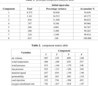
, material speed_(x5), permeability_(x6), coal injection_(x7) and oxygen enrichment rate_(x8),. The PCA was carried out by using SPSS 22, and the results were shown in table 1.

training speed of the LSSVM. Extracting those 4 principal components, the resulting component matrix is shown in table 2.

Table 1. principal component analysis table

Component

Initial eigenvalue

Total Percentage variance Accumulate %

1 4.373 54.658 54.658

2 1.161 14.515 69.173

3 .916 11.450 80.623

4 .747 9.344 89.966

5 .384 4.801 94.767

6 .280 3.498 98.265

7 .124 1.549 99.814

8 .015 .186 100.000

Table 2. component matrix table

Variables Component

1 2 3 4

air volume .907 .159 .009 -.248

wind temperature .486 -.248 .629 .537

wind pressure .913 -.144 -.179 .148

top pressure .933 -.131 -.184 .104

material speed .857 .039 -.159 -.190

permeability .462 .565 .580 -.318

coal injection .332 .736 -.304 .453

oxygen enrichment rate .742 -.417 -.014 -.147

From the component matrix of Table 2, we can derive 4 principal component equa-tions:

1 1 2 3 7 8

2 1 2 3 7 8

3 1 2 3 7 8

4 1 2 3 7 8 0.907 0.486 0.913 0.332 0.742

0.159 0.248 0.144 + 0.736 0.417 0.009 0.629 0.179 + 0.304 0.014 0.248 0.537 0.148 0.453 0.147

F x x x x x

F x x x x x

F x x x x x

F x x x x x

= + + + + +

!

" _{= # # + #} "

$ _{= + # # #} "

" =# + + + + # %

! ! ! !

(16)

From the component matrix, the PCA method has a good effect on reducing di-mension. Among them, the first principal component is a linear combination of five variables, which is highly related to air volume, air pressure, top pressure, material speed and oxygen enrichment rate. Besides, the other three principal components are highly correlated with two variables. The second principal component is highly relat-ed to coal injection and permeability. The third principal component and the fourth principal components explained mainly two variables, air temperature and permeabil-ity. In summarywe can understand that the first principal component is a

pressure, feed rate and oxygen enrichment rate linear representation. The second prin-cipal component is a mixing factor relating to coal injection and permeability. The third and fourth principal components are the mixing factors of wind temperature and coal injection. To sum up, we can redefine the new four variables: Z1=F1; Z2=F2;

Z3=F3; Z4=F4, we set the new four variables as input variables of LSSVM algorithm.

3.3 LSSVM’s analysis

In this paper, two sets of training sets are selected from 1108 blast furnace samples. The first training set is blast furnace numbered from 1 to 450, and the second one is 631 to 980. The corresponding test set is from 461 to 500 and from 981 to 1020, re-spectively. At the same time, we set 12 times cross validation to confirm the parame-ters

!

and

!

2_{. It can ensure each subset has enough space to illustrate its effectiveness}

in cross validation and the reliability of the study. Figure 1 shows the observation of ([Si]) in 1108 original blast furnace in the blast furnace system number value.

Fig. 1. Observation of ([Si]) in blast furnace

In the previous PCA, we use four principal components instead of the original eight variables as input variables. These four input variables can be defined as

) ~ , ~ , ~ , ~ ( ) , , ,

( 1 2 3 4

4 3 2

1 Z Z Z z z z z z

Z = = ₍₁₇₎

The PCA shows that the principal components are independent of each other, so the correlation coefficient between the four principal components is 0 and linearly independent. Therefore the relationship between variables can be eliminated.

With different dimension, these data need to be manipulated before being ana-lyzed. In general, we use the normalization method to fix all variables between 0 and 1, and the formula of normalization is as follows:

0 200 400 600 800 1000 0.4

0.6 0.8

Heat No.

[S

i] M

as

s F

rac

tion

( )

( )

( )

{

}

{

}

! ! ! " ! ! ! # $ = = = = = = % % = 1108 , 2 ,1 ~ min ) ~ min( 1108 , 2 ,1 ~ max ) ~ max( 4 , 2 ,1 ; 1108 , 2 ,1 , ~ min ~ max ~ min ~ ! ! ! ! i z z i z z j i z z z z z j i j j i j j j j j i j i (18) j i

z

~

_{can be performed as observations.}

Thus, all the data can be normalized and the dimensional influence eliminated by the above formula.

After we processed treatment

(

1

,

2

,

3

,

4

)

i i i i

i

z

z

z

z

z

=

, which used as input variables

of LSSVM, then the ([Si]) content can be seen as the output variable. We Select the RBF kernel as the kernel function

k

(

x

_i

,

x

_j

)

and use 12-fold cross validation for choosing the hyper parameters according to the former procedure. This is done through the LSSVM-lab 1.8 package Toolkit. After this, we estimated two groups of parameters for training set: (

"

1,

!

1)=(10.35,0.58)and(

"

2,

!

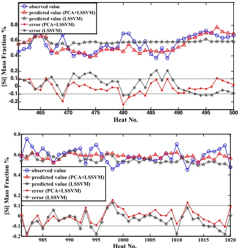
2)=(8.38,0.35).Finally, we

predict the ([Si]) of the two sets of tests, which is shown in Figure 2. Figure 2 shows the comparison between the observed and predicted values of ([Si]) in the two sets of tests. It illustrates that the prediction of LSSVM algorithm based on PCA is better than using LSSVM algorithm.

Fig. 2. Comparison of predicted and observed values of two sets of test sets

465 470 475 480 485 490 495 500 -0.2 -0.1 0 0.1 0.2 0.4 0.6 0.8 Heat No. [S i] M as s F rac tion % observed value

predicted value (PCA+LSSVM) predicted value (LSSVM) error (PCA+LSSVM) error (LSSVM)

985 990 995 1000 1005 1010 1015 1020 -0.2 -0.1 0 0.1 0.2 0.4 0.6 0.8 Heat No. [S i] M as s F rac tion % observed value

In addition, the standard of evaluation model can be reflected by the following two indicators:

(1) RMSE-Root mean square error Define the root mean square error

2 / 1 2

1

] ) ˆ ( 1 1

[ i

n

i yi y n

RMSE ! !

=

"

= (19)

Where

y

ˆ

_iis the predicted value,

y

_iis the observed value,

n

is the length of the pre-dicted data set. The range of RMSE is between 0 and 1. If RMSE is closer to 0, this model provide a better prediction result.

(2) PHT-Percentage of hitting target Define the percentage of hitting target

%

100

1

1

!

=

"

= n

i i

H

n

PHT

#

(20)

i

H

means hit count, it can be written as:

! "

# % $

=

otherwise y y H i i

i

! !

! !

0 ˆ

1

&

(21) Where

y

ˆ

_{i is the predicted value,}

y

_iis the observed value,

n

is the length of the pre-dicted data set.

H

_itakes only two values:0 or 1,If _{Hi =1},it conveys that the observed and predicted values of this sample are within the range of error. On the contrary,

0

= i

H , beyond the range of error.

!

reflects the difference between observed and predicted values. It is a small positive number, Normally,

!

takes 0.1.The PHT value is between 0 and 1. Generally speaking, when PHT value is greater than 0.8, the mod-el prediction simulation provides a positive result..

Table 3 reflects. It is can be found that the composite model provides more accura-cy than single model which applied LSSVM only.

Table 3. prediction results of ([Si])

Test set Basic methods RMSE Hits PHT

461-500 LSSVM 0.103 25 0.625

PCA+LSSVM 0.082 32 0.8

981-1020 LSSVM 0.084 29 0.725

4

Conclusions

In this paper, a new algorithm formed up by combining PCA and LSSVM is used to predict [Si] in Blast Furnace System. The simulation shows that the new method achieves more obvious prediction hit rate than the direct multivariable LSSVM, which indicates that 80% vs 62.5% and 87.5% vs 72.5% respectively. The new algo-rithm has positive significance. Furthermore, when the continuous sampling is insuf-ficient (learning data segments), the new algorithm has better stability than the direct algorithm.

5

Acknowledgements

This research is partially supported by the NSFC (61563018), the NSF of Jiangxi Province 20161ACB20009, 20133BCB23014) and the Foundation of the Office of Education, Jiangxi Province (KJLD13033).

6

References

[1]Ueda, S, Natsui S, Nogami H, Yagi J.I!and A. Tatsuro: Recent progress and future per-spective on mathematical modeling of blast furnace [J]. ISIJ Int., 2010, 50(7), pp. 914-923. https://doi.org/10.2355/isijinternational.50.914

[2]X. G. Liu and F. Liu: Optimization and Intelligent Control System of Blast Furnace Iron-making Process, Metallurgical Industry Press, Beijing, (2003).

[3]X.Y. Liu: Research on [Si] predictive control model of blast furnace temperature based on Bayesian network [D]. Master's degree thesis of Zhejiang University, 2004.

[4]C.H. Gao, Z.M. Zhou, Z.J. Shao: Chaotic Local-region Linear Prediction of Silicon Con-tent in Hot Metal of Blast Furnace [J]. Acta Metall. Sin., 2005, 41: 433-436.

[5]M. Zhao, X.G. Liu, S.H. Luo: An Evolutionary Artificial Neural Networks Approach for BF Hot Metal Silicon Content Prediction Based on Chaotic Analysis [J]. LNCS (Lecture Notes in Computer Science), 2005, (3610): 572-575.

[6]H.W. Guo, L.K. Chen, H.B. Zuo, T.J. Yang: Prediction model of blast furnace temperature based on fuzzy reasoning [J]. Iron and steel research, 2007, 35 (2): 22.

[7]H.W. Guo, L.K. Chen, H.B. Zuo, T.J. Yang: Application of multidimensional time series fuzzy association rules to prediction of blast furnace temperature [J]. Journal of University of Science and Technology Beijing, 2008, 30 (5): 553.

[8]Bhattacharya. T, Prediction of silicon content in blast furnace hot metal using partial least squares (PLS). ISIJ International, 2005, 45(12): 1943-1945. https://doi.org/10.2355/isijin ternational.45.1943

[9]M.S. Chu, X.Z. Guo, F.M. Shen: Blast furnace mathematical model and solution based on Multi fluid theory [J]. Northeastern University (NATURAL SCIENCE EDITION), 2007, 28 (3): 361.

[10]L. Jian, C.H. Gao, and Z.Q. Xia, “A sliding-window smooth support vector regression model for nonlinear blast furnace system,” Steel. Res. Int., 2011, 82(3), pp. 169-179. https://doi.org/10.1002/srin.201000082

[12]S.W. Xie: Principal component analysis and factor analysis of mathematical model based on the application of [D]. Shandong University of Technology, 2016.

[13]P. Wang, Y.W. Deng, Y.P. Tian, F.M. Kuang, F. Yi: Hengyang City, the land ecological security evaluation based on principal component analysis [J]. Economic geography, 2015 (01): 168-172.

[14]W. Lei: Support vector machine regression prediction model based on principal compo-nent analysis [J]. Information technology, 2008, (12): 58-60.

[15]R.N. Shen, C. Cao, C.J. Fan: Practice and understanding principal component analysis and support vector machine model of Shanghai price prediction research [J]. mathematics, 2013, (23): 11-16.

[16]V. N. Vapnik, The Nature of Statistical Learning Theory, Springer-Verlag, New York, NY, USA, 2nd edition, 2000. https://doi.org/10.1007/978-1-4757-3264-1

[17]J.H. Zheng: Research on prediction of blast furnace temperature based on support vector machines [D]. Zhejiang University, 2007.

[18]J. Liu, J. Chen, S. Jiang, and J. Cheng : Online LS-SVM for function estimation and classi-fication [J]. Univ. Sci. Technol. B., vol. 10, no. 5, 2003.

[19]C. Gao, L. Jian, and S.H. Luo, “Modeling of the thermal state change of blast furnace hearth with support vector machines,” IEEE Transactions on Industrial Electronics, vol. 59, no. 2, pp. 1134–1145, 2012. https://doi.org/10.1109/TIE.2011.2159693

[20]L.H. Wang, S. Gao, X. Qu: Prediction of silicon content in molten iron in LSSVM blast furnace based on GA optimization [J]. Journal of Terahertz Science and electronic infor-mation, 2013, (04): 641-645.

[21]Y. Tao: Application and improvement of blast furnace temperature prediction using LSSVM [D]. Shenyang University of Aeronautics and Astronautics, 2014.

[22]Y.J. Yue, Y.F. Lu, Hui. Z, H.J. Wang: Prediction of blast furnace gas using wavelet analy-sis ARIMA and LSSVM [J]. Computer measurement and control, 2015, (06): 2128-2131. [23]Y.T. Xiong, Z.P. Li, J.Wang, S.W. Feng, Z.W. Li, J.J. Yin, Q.H. Song: Analysis of liquor

grains quantitative composition based on least squares support vector machine. Food sci-ence, 2016,37 (12): 163-168.

[24]Y.J. Yue, Y.F. Cheng , H. Zhao, H.J. Wang: Prediction of blast furnace gas based on wavelet analysis ARIMA and LSSVM computer measurement and control [J]. 2015,23 (06): 2128-2131.

[25]C. Zhao, K.C. Dai: Short term power load forecasting based on adaptive weighted least squares support vector machines [J]. information and control, 2015,44 (05): 634-640. [26]R.X. Li: Approximate Lagrange multipliers and KKT conditions for constrained vector

op-timization [D]. Yunnan University, 2013.

7

Authors

Tianxin Chen is currently an Postgraduate of School of Statistics, Center of Ap-plied Statistics, Jiangxi University of Finance and Economics, Nanchang, 330013, China. He received the B.S. degree in Statistics from Lanzhou University of Finance and Economics, China, in 2012 and 2016. His research interests are multivariate sta-tistical analysis, data mining and machine learning algorithms.

Ling Jian is currently an Associate Professor, where he has been with the School of Science, China University of Petroleum, Qingdao, 266555, China since March 2006. He received the B.S. degree in applied mathematics from Qufu Normal Univer-sity, Qufu, China, in 2003, the M.Sc. degree in operational research and cybernetics from Zhejiang University, Hangzhou, China, in 2006 and the Ph.D. degree in opera-tional research and cybernetics from the Dalian University of Technology, Dalian, China, in 2012. His scientific interests include machine learning, data mining, kernel methods and optimization.