Modelling soil water dynamics and root water uptake for apple trees
under water storage pit irrigation
Xianghong Guo
,
Tao Lei
*,
Xihuan Sun
,
Juanjuan Ma
,
Lijian Zheng
,
Shaowen Zhang
,
Qiqi He
(College of Water Resource Science and Engineering, Taiyuan University of Technology, Taiyuan 030024, China)
Abstract: Water storage pit irrigation is a new method suitable for apple trees. It comes with advantages such as water saving, water retention and drought resistance. A precise study of soil water movement and root water uptake is essential to analyse and show the advantages of the method. In this study, a mathematical model (WSPI-WR model) for 3D soil water movement and root water uptake under water storage pit irrigation was established based on soil water dynamics and soil moisture and root distributions. Moreover, this model also considers the soil evaporation, pit wall evaporation and water level variation in the pit. The finite element method was used to solve the model, and the law of mass conservation was used to analyse the water level variation. The model was validated by experimental data of the sap flow of apple trees and soil moisture in the orchard. Results showed that the WSPI-WR model is highly accurate in simulating the root water uptake and soil water distributions. The WSPI-WR model can be used to simulate root water uptake and soil water movement under water storage pit irrigation. The simulation showed that orchard soil water content and root water uptake rate centers on the storage pit with an ellipsoid distribution. The maximum distribution region of soil water and root water uptake rate was near the bottom of the pit. Distribution can reduce soil evaporation in the orchard and improve the soil water use efficiency in the middle-deep soil.
Keywords: root water uptake, soil water dynamics, numerical simulation, water storage pit irrigation, apple tree DOI: 10.25165/j.ijabe.20191205.4005
Citation: Guo X H, Lei T, Sun X H, Ma J J, Zheng L J, Zhang S W, et al. Modelling soil water dynamics and root water uptake for apple trees under water storage pit irrigation. Int J Agric & Biol Eng, 2019; 12(5): 126–134.
1 Introduction
Soil water movement and root water uptake are the key processes of the substance transport and energy transfer in farmland[1–3]. A quantitative study of soil water and root is the
basis of formulating irrigation system and improving water use efficiency. Soil moisture and root interact restrict each other, root water uptake is the main method for soil moisture consumption in the root zone. On the other hand, soil moisture is the main factor that restricts root water uptake[4-6]. A reasonable distribution of
soil moisture in the root zone can promote root water uptake and improve water use efficiency.
Water storage pit irrigation is a new method for simultaneously solving the problems of drought and soil erosion. Water storage pit irrigation with the advantages of water saving, water retention, drought resistance and soil and water conservation is suitable for apple trees[7-10]. In the field, several small cylindrical storage pits
(pit diameter 25-30 cm and pit depth 40-60 cm) are dug along half of the radius of the apple tree canopy. During irrigation, water flows into the annular groove through the pipeline or field channel,
Received date: 2017-11-27 Accepted date: 2019-07-17
Biographies: Xianghong Guo,PhD, Professor, research interest: water saving irrigation, Email: xianghong7920@126.com; Xihuan Sun, PhD, Professor, research interest: water saving irrigation, Email: sunxihuan@tyut.edu.cn;
Juanjuan Ma,PhD, Professor, research interest: water saving irrigation, Email: majuanjuan@tyut.edu.cn; Lijian Zheng, PhD, research interest: water saving irrigation, Email: 984106887@qq.com; Shaowen Zhang, MS, research interest: water saving irrigation, Email: 1332163437@qq.com; and Qiqi He, MS, research interest: water saving irrigation, Email: 552925194@qq.com.
* Corresponding author: Tao Lei, PhD, research interest: water saving irrigation. College of Water Resource Science and Engineering, Taiyuan University of Technology, Taiyuan 030024, China. Tel.: +86-18334703862, Email: 1046677432@qq.com.
then enters the pits and infiltrates into the rhizosphere soil along the pit wall. During water storage pit irrigation, the soil infiltration interface changes. The water content in middle-deep soil is high, whereas that in topsoil is low. Water content is different in surface, sprinkler and micro irrigations. The distribution of soil moisture under water storage pit irrigation can reduce ground evaporation between plants, boost the growth of roots in middle-deep soil, change the distribution of root system and promote the root water uptake[11-14].
The mathematical model of soil water movement under root water uptake can be built by adding the root water uptake item to the right end of the basic equation of soil water movement, while considering boundary conditions such as irrigation, evaporation and rainfall. In general, the root water uptake model has two types, namely, micro and macro models[15]. The macro model is more
common than the micro model, and the macro model can be subdivided into two categories[16]: the first category is built by
distributing plant transpiration to different soil depths according to root density, and the second category is built on the basis of the spatial distribution of root water uptake intensity, which is obtained by the soil water dynamics. By contrast, the first category is easier and more popular than the second category. In recent years, many mathematical models for orchard soil water movement and root water uptake have been developed. Most of the models are 1D[17-19] or 2D[20-22], only a few are 3D[23]. Numerical solutions,
such as finite difference, finite element and finite volume methods, were adopted to solve the models[24-28]. Finite element method is
widely used because of its favourable adaptability to irregular boundary conditions. Hydrus 2D/3D is developed based on the finite element method[29]. This software performs well in
simulating water-heat-solute transport in farmland[30,31]. However,
infiltration head and infiltration area that act on the pit wall infiltration interface during water storage pit irrigation declines with infiltration time. Moreover, the infiltration head has a wide range of variation. The soil water movement under water storage pit irrigation is 3D. Thus, factors such as root water uptake and complex boundary conditions must be considered in the simulation.
This study aims to establish the soil water movement and root water uptake model (WSPI-WR model) for apple trees under water storage pit irrigation, calibrate and validate the model by using the measured data in the orchard and show the spatial distribution characteristics of soil moisture and root water uptake through water storage pit irrigation method.
2 Materials and methods
2.1 Study area
The field study was conducted at the Fruit Research Institute of Shanxi Academy of Agricultural Sciences (latitude 37°23′N, longitude 112°32′E) from May 23rd to October 10th, 2013. The
region is located in the southwest of Taigu County, Shanxi Province. The region has a typical temperate continental climate with a long-term annual mean air temperature and precipitation of 9.8 °C and 462.9 mm, respectively. The frost period is from early October to mid-April of the following year, and the frost-free period spans 175 d. The area of the region is 450 ha, and the soil type is mainly loam. The apple trees (Malus pumila Mill) discussed in this study were planted with a row and plant spacing of 4 and 2 m, respectively.
2.2 Experimental design and test items 2.2.1 Experimental design
The field engineering of water storage pit irrigation included storage pits, annular groove, conveyance ditch (or a delivery pipe) and facilities to firm the pit wall (Figure 1). The storage pit (diameter 30 cm and pit depth 60 cm) was arranged under the crown and 60 cm away from the trunk. Four storage pits are under each apple tree. The bottom of the pit was waterproofed to reduce deep percolation, and metal mesh was used to firm the pit wall. The annular groove (depth 20 cm and width 30 cm) was used to connect all the storage pits around the tree. The delivery pipe is a fixed field pipe that connects the irrigation backbone system with the annular groove. Water flowed into the annular groove through the delivery pipe during irrigation and then entered the pits and infiltrated into the soil through the pit wall. The irrigation events were conducted on May 23rd and September 11st,
2013. The irrigation quota per tree was 300 L.
Figure 1 Field engineering diagram of water storage pit irrigation 2.2.2 Measurement of soil moisture content
Soil moisture content was measured using the TRIME-PICO IPH measuring system every 5-10 d. An additional measurement should be performed after rain or irrigation. Figure 2 illustrated
the layout of the measuring points. The measuring depth was 200 cm, and the vertical measurement spacing was 20 cm.
Figure 2 Layout of the measuring points of the soil moisture and root
2.2.3 Measurement of soil evaporation
The orchard soil evaporation under water storage pit irrigation, included the pit wall and surface evaporations, was measured using micro-lysimeters[32]. Micro-lysimeters were arranged along the
pit wall. Figure 3 depicts that each storage pit requires three micro-lysimeters with depths of 10, 30 and 50 cm. Figure 4 displays that micro-lysimeters for surface evaporation were arranged under the crown 50, 100 and 150 cm away from the trunk.
Figure 3 Diagram of the pit wall evaporation test
Figure 4 Diagram of the surface evaporation test 2.2.4 Measurement of sap flow rate of the apple tree
The sap flow rate of the apple tree was measured by using a thermal diffusion probe sap flow meter (TDP, Dynamax Company, USA). Waterproof daub was applied at the junction of the probe and bark, and aluminium film and silver paper were wrapped around the trunk to eliminate the influence of the sun on the thermal probe. The end of the probe was connected to a data collector, and data were collected and recorded every 15 s and 30 min, respectively.
2.2.5 Measurement of root length density
considered as the centre, and the measuring points were placed 30, 60, 90 and 120 cm away from the trunk (Figure 2). The soil samples were collected at a depth interval of 20 cm. The total sampling depth was 200 cm. Soil samples with roots were removed, immediately placed in sealed plastic bags and then transported back to the laboratory. The roots were tiled in organic glass dishes (20 cm × 25 cm) after washing and separation using clean water and tweezers, and no overlap existed among the roots. Subsequently, the roots were scanned using an Epson Perfection 4870 scanner. Finally, software WinRHIZO (Regent Instruments, Canada) was used to analyse the scanned results and obtain the root length density.
2.2.6 Measurement of leaf area index (LAI)
Leaf area index (LAI) was measured monthly from May 2013 to September 2013 using a LAI-2200 vegetation canopy analyser (LI-COR, USA).
2.2.7 Collection of meteorological data
Meteorological data, including precipitation, atmospheric temperature, soil temperature, wind speed, wind direction, pressure atmosphere, relative humidity and solar radiation, were collected from the Adcon_Ws weather station every 15 min. Figure 5 presents the variation of precipitation and reference crop evapotranspiration (ET0) during the experiment.
Figure 5 Variation of precipitation and ET0 during the experiment
2.3 Soil water movement and root water uptake model under water storage pit irrigation
2.3.1 Governing equation
Three-dimensional features are obvious in soil water movement under water storage pit irrigation. The computational region was determined according to the symmetrical placement of storage pits (Figure 6). The 3D equation of water movement that considers root water uptake was expressed as Equation (1).
( )
[ ( ) ] [ ( ) ] [ ( ) ]
θ h h h K h
K h K h K h S
t x x y y z z z
∂ ∂ ∂ ∂ ∂ ∂ ∂ ∂
= + + + −
∂ ∂ ∂ ∂ ∂ ∂ ∂ ∂
(1) where, h is the soil water pressure, cm; K(h) is the unsaturated hydraulic conductivity, cm/h; x, y and z are the space coordinates, cm; t is time, h; and S is the root water uptake rate, L/h.
The soil hydraulic properties were modelled using van Genuchten-Mualem constitutive relationships (van Genuchten, 1980), as defined in Equations (2) and (3).
0
( ) [1 ]
0
s r h
r n m
h h
h s
θ θ θ
θ α
θ
−
⎧ + <
⎪
=⎨ +
⎪ ≥
⎩
(2)
and
1/2[1 1/ ]2 0
( )
0 m
K Ss e Se h
K h
Ks h
⎧⎪ − <
=⎨
≥
⎪⎩ (3)
where, Se=(θ–θr)/(θs–θr); m=1–1/n; θs is the saturated water content, cm3/cm3; θr is the residual water content, cm3/cm3; and Ks
is the saturated hydraulic conductivity, cm/h.
Figure 6 Computational region of water storage pit irrigation In order to run model, the hydraulic parameters θs, θr, Ks, α and n were measured by specific experimental methods. First, a soil profile with length 2.0 m, width 1.0 m and depth 2.0 m was excavated at the experimental site. Then, according to the soil texture, color, tightness, etc., the soil profile was divided into 5 layers 0-40 cm, 40-70 cm, 70-120 cm 120-170 cm and 170-200 cm, and six soil samples were collected in each layer of soil using soil cutting ring. Then the soil samples were brought back to the laboratory and the soil water content corresponding to different pressures was measured using a 1500F1 pressure plate extractor (Soilmoisture Equipment Corp., Goleta, CA, US). According to the measured soil water content and pressure data, the equation (2) was fitted with MALAB2016 and the values of parameters θs, θr, α and n were obtained. The saturated hydraulic conductivity Kswas measured by a TST-55 permeameter (Nanjing Soil Instrument Co., Ltd., China). Table 1 lists the soil hydraulic parameters.
Table 1 Soil hydraulic parameters of experimental plot soil
Depth/cm Ks/cm·h-1 θr/cm3·cm-3 θs/cm3·cm-3 α n
0-40 0.522 0.0545 0.51 0.0071 1.5801 40-70 0.768 0.0536 0.52 0.0008 1.5552 70-120 0.684 0.0496 0.49 0.0085 1.5296 120-170 0.606 0.0465 0.50 0.0094 1.5243 170-200 0.888 0.0443 0.52 0.0091 1.5419
The root water uptake term in Equation (1) is presented in Equation (4)[23].
max
( , , , ) ( ) ( , , , )
S x y z t =γ h S x y z t (4) where, γ(h) is the coefficient of water stress (Equation (5)), and Smax is the maximum root water uptake rate (L/h) (Equation (6))[23].
0
1 0
0 1
2 1
3
3 2
2 3
3
1 ( )
0
h h
h h h
h h
h h h
γh
h h h h h
h h
h h
−
⎧ ≤ ≤
⎪ − ⎪
≤ ≤ ⎪
= ⎨ −
⎪ ≤ ≤
⎪ −
⎪ ≤
⎩
where, h0, h1, h2, h3 are thresholds of soil water potential that
affects root water uptake. For the apple tree, h0, h1, h2, h3 are 0,
−0.1, −10 and −150 m, respectively[18].
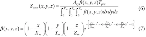
max
0 0 0
( , , ) ( , , )
( , , )
m m m
xy pot
X Y Z
A β x y z T
S x y z
β x y z dxdydz
=
∫ ∫ ∫
(6)* * *
| | | | | |
( , , ) 1 1 1
y
x z
m m m
p
p x x y y p z z
X Y Z
m m m
x y z
β x y z e
X Y Z
⎡ ⎤
−⎢ − + − + − ⎥
⎣ ⎦
⎛ ⎞⎛ ⎞⎛ ⎞
=⎜ − ⎟⎜ − ⎟⎜ − ⎟
⎝ ⎠⎝ ⎠⎝ ⎠ (7)
where, Tpot is the potential transpiration intensity (cm/d) (Equation (8))[15]; β(x, y, z) is the function of root distribution shape; X
m, Ym,
Zm are the maximum extension depths (cm) of root in x, y and z
directions, respectively; Axy is the area of computational region on the surface, cm2; and px, py, pz, x*, y*, z* are the fitting parameters of
Equation (7) using the measured root length density (Table 2). Table 2 Parameters of the root water uptake model
px py pz x*/cm y*/cm z*/cm
1.81 1.02 1.82 103.48 52.38 82.23
{1 |sin[( 13) /12]|} 0
( ) ( )(1 kLAI A t π ) ( )
pot
T t = a bLAI+ −e− + − ET t
(8) where, LAI is the leaf area index; a, b, k and A are constants with values of 0.2432, 0.448, 0.402 and 0.976, correspondingly[20]; and
ET0 is the reference crop evapotranspiration calculated using the
Penman-Monteith formula[33].
2.3.2 Initial condition
h(x,y,z,t)=h0(x,y,z) t=0 (9)
where, h0(x,y,z) is the suction head that corresponds to the initial
water content, cm.
2.3.3 Boundary conditions
1) Surface boundary (AQJ, MEDL and PIRFN)
For surface boundary, the upper boundary is considered the second boundary when precipitation intensity is less than infiltration intensity; the upper boundary is transformed from the second boundary into the first boundary when precipitation intensity is higher than infiltration intensity, and excess rainfall becomes surface runoff and flows into the water storage pit (Equations (10) and (11)).
( ( )K h h K h( )) P P i z
∂
− + = <
∂ (10) ( , , ) s
h x y z =h P i> (11) where, P is the net precipitation intensity, cm/h; i is the infiltration intensity, cm/h; zu is the z coordinate value of the surface boundary
and hs is the surface ponding depth, cm.
The upper boundary is the second boundary during evaporation; the upper boundary is transformed into the first boundary when the ground becomes dry.
( ( ) ( )) s ( , , )u d
h
K h K h e h x y z h
z
∂
− + = >
∂ (12)
( , , ) d ( , , )u d
h x y z =h h x y z ≤h (13) where, es is the surface evaporation intensity, cm/h; and hd is the suction head when the ground is dry, cm.
2) Lateral wall boundary of the annular groove (EFNM and
QJIP)
The lateral wall boundary of the annular groove is the second boundary during evaporation; the boundary is transformed into the first boundary when the ground becomes dry.
( )( x y) s ( , , ) d
h h
K h n n e h x y z h
x y
∂ ∂
− + = >
∂ (14)
( , , ) d ( , , ) d
h x y z =h h x y z ≤h (15) where, nx, ny are the components of the normal vector.
3) Pit wall boundary (IRFGOH)
The pit wall boundary is the first boundary during irrigation. h(x, y, z)=hi (16) where, hi is the pressure head of each point on the pit wall, which has the value of the distance from the point to the water level in the pit.
The pit wall boundary is considered the second boundary when the infiltration in the pit is completed.
( )( x y) s
h h
K h n n e
x y
∂ ∂
− + =
∂ (17) 4) Pit bottom boundary (HOG)
The pit bottom boundary is impermeable.
( ( )K h h K h( )) 0 z
∂
− + =
∂ (18) 5) Lower boundary (BCK)
The lower boundary is considered a free drainage boundary given the deep calculation depth and bury of groundwater.
h(x, y, z)=h0 (19)
6) Boundary ABCD
Boundary ABCD is considered a zero flux plane because of its symmetry.
( ) h 0
K h x
∂
− =
∂ (20) 7) Boundary ABKL
Boundary ABKL is also considered a zero flux plane because of its symmetry.
( )( x y) 0
h h
K h n n
x y
∂ ∂
− + =
∂ (21) 8) Boundary CDLK
No horizontal water exchange is assumed for boundary CDLK because of the large calculation area.
( ) h 0
K h x
∂
− =
∂ (22) 2.3.4 Model solving
This study uses the Galerkin finite element method to solve the 3D Richards equation because the finite element method is easy to use under complex boundary conditions. The flow region was divided into a network of tetrahedral elements (Figure 7). Equation (1) is solved by using the finite element method with the Galerkin weighted residual method.
{ }
[ ]{ } [ ]A h G θ { } { } { }Q B D t
∂
+ = − −
∂ (23)
where, {h}=[h1, h2, …, hn]T.
2 2 2
2 2 2
2 2 2
[ ] 36
i i i i j i j i j i k i k i k i m i m i m
j i j i j i j j j j k j k j k j m j m j m
e
e k i k i k i k j k j k j k k k k m k m k m
m i m i m i m j m j m j m
b c d b b c c d d b b c c d d b b c c d d
b b c c d d b c d b b c c d d b b c c d d
K A
V b b c c d d b b c c d d b c d b b c c d d
b b c c d d b b c c d d b
+ + + + + + + + + + + + + + + + = + + + + + + + + + + + +
∑
2 2 2
k m k m k m m m
b c c d d b c d
where, 1[ ]
4 i j k m
K= K +K +K +K .
1 1 1
1 1 1
1 1 1
1 1 1
1 1 1
1 1 1
1 1 1
1 1 1
1 1 1
1 1
1 1
j j j j j j
i k k i k k i k k
m m m m m m
i i i i i i
j k k j k k j k k
m m m m m m
i i i i i i
k j j j k k j k k
m m m m m m
i i i
m j j m
k k
y z x z x y
b y z c x z d x y
y z x z x y
y z x z x y
b y z c x z d x y
y z x z x y
y z x z x y
b y z c x z d x y
y z x z x y
y z x
b y z c
y z = = = = = = = = = = = 1 1 1 1 1
i i i
j j m j j
k k k k
z x y
x z d x y
x z x y
= (25) 1 1 [ ] 1 4 1 e e V G ⎡ ⎤ ⎢ ⎥ ⎢ ⎥ = ⎢ ⎥ ⎢ ⎥ ⎣ ⎦
∑
(26){ } 6 i j k e m d d K B d d ⎛ ⎞ ⎜ ⎟ ⎜ ⎟ = ⎜ ⎟ ⎜ ⎟ ⎝ ⎠
∑
(27)0 1 { } 1 3 1 e e L Q q ⎛ ⎞ ⎜ ⎟ ⎜ ⎟ = − ⎜ ⎟ ⎜ ⎟ ⎝ ⎠
∑
(28)2 2 { } 2 20 2
i j k m
e
i j k m
i j k m
e
i j k m
S S S S
S S S S
V D
S S S S
S S S S
+ + + ⎡ ⎤ ⎢ + + + ⎥ ⎢ ⎥ = − ⎢ ⎥ + + + ⎢ ⎥ + + + ⎢ ⎥ ⎣ ⎦
∑
(29)where, i, j, k and m are the node numbers of the tetrahedral element e, Ve is the volume of element e, and K is the average hydraulic conductivity over element e. Le is the area of flux boundaries in tetrahedral elements (cm2), and q is the flux on the flux boundary
of the tetrahedral element (cm3/min). Equation (28) is only
significant to the flux boundary. The internal and Dirichlet boundary nodes are 0, and the boundary of the tetrahedron element is jkm, which is the area of the interface jkm.
Figure 7 Mesh generation results
An implicit backward difference scheme is used for the time term in Equation (23).
0 0
0 0 0 0 0
0
1
1 1 1
{ } { }
[ ] [ ] { } { } { } { }
Δ
j j
j j j j j
j
θ θ
G A h Q B D
t
+
+ + +
− + = − −
(30)
where, j0+1 denotes the current time level at which the solution is
considered, j0 refers to the previous time level and Δtj0=tj0+1–tj0. The ‘mass conservation’ method[34] was adopted to handle the
water content term ( t
θ Δ
Δ ); the first item in Equation (30) was divided into the following parts in the iterative process:
0 0 0
0
0 0 0 0 0
0 0 0
1
1 { } 1 { } 1 { } 1 { }
{ } { }
[ ] [ ] [ ]
Δ Δ Δ
k k k
j
j j j j j
j j j
θ θ θ θ
θ θ
G G G
t t t
+
+ − = + − + + + − (31)
The first term on the right-hand side can be expressed in terms of pressure head; thus, Equation (31) becomes the following one:
0 0 0
0
0 0 0 0 0 0
0
0 0 0
1
1 1 1 1
1
{ } { } { } { }
{ } { }
[ ] [ ][ ] [ ]
Δ Δ Δ
k k k
j
j j k j j j
j
j j j
h h θ θ
θ θ
G G C G
t t t
+ + + + + + − − − = + (32) Equation (33) will be obtained by substituting Equation (32) into Equation (30), as follows:
0 0
0 0 0 0 0
0 0 0
0 0
0 0
0 0
0 0 0
0
1 1 1
1 1 1
1 1 [ ][ ] [ ][ ] [ ] { } { } Δ Δ { } { } [ ] { } { } { } Δ k k
j k k j k
j j j
j j
k j
j k
j j j
j
G C G C
A h h
t t
θ θ
G Q B D
t + + + + + + + + ⎛ ⎞ + = − ⎜ ⎟ ⎜ ⎟ ⎝ ⎠ − + − − (33)
2.3.5 Solution of water depth changing process in the water storage pit
The water level in the pit continuously declines during water storage pit irrigation, and the boundary conditions of the pit wall continuously change with time. Therefore, an accurate calculation of water level-changing process in the pit is the key step in the numerical simulation of soil water movement. According to the principle of mass conservation, the amount of water that reduces in the pit is equal to the amount of water that infiltrates into the soil by the pit wall during irrigation (Equation (34)).
0 | |
t
t n
n
Vol Vol− =
∫
∑
Q dt′ (34)where, Vol is the amount of irrigation water in a single pit, cm3;
Voltis the amount of water in a single pit at time t (cm3) (Equation (36)); and Q′n is the boundary section flow controlled by the node n on the pit wall boundary, which is the product of the flow of the boundary node and the area of the control boundary section.
N equations will be obtained by substituting the head value into Equation (33) when the real-time head value {h} of each node t is calculated. The node n on the boundary of the pit wall corresponds to the nth equation of N equations, in which Qn (the nth of {Q}) is unknown, and the remaining nodes are known. Q′n can be calculated using Equation (35) as follows:
0 0
0 0 0 0
1
1 1 1
1 1
( )
Δ
j j
N N
m m j j j j
n nm m n n
m m
θ θ
Q Gnm A h B D
t
+
+ + +
= =
−
′ = −
∑
+∑
+ + (35)where, N is the total number of nodes in the calculation region. Volt=πr0Ht (36)
where, Ht is the water depth in the pit at moment t, cm.
Equation (37) will be obtained by substituting Equations (35) and (36) into Equation (34), as follows:
0 0
0 0 0 0
1
1 1 1
0 1 1
0
Δ
j j
N N
t m m j j j j
nm m n n
n m m
t
θ θ
Vol Gnm A h B D dt
belongs to the first boundary when this point is below the water level; the boundary point belongs to the second boundary when this point is above the water level.
2.3.6 Model evaluation
The root-mean-square error (RMSE), maximum relative error (MRE), average relative error (ARE) and mean absolute error (MAE) were used to evaluate the model (Equations (38)-(41)).
2
1
( s R)
l
i i
i
V V
RMSE
l
=
−
=
∑
(38)1
max l is iR 100%
R
i i
V V
MRE
V
=
⎛ − ⎞
= ⎜⎜ × ⎟⎟
⎝
∑
⎠ (39)1
1
100%
s R
l
i i
R
i i
V V
ARE
l = V
−
=
∑
× (40)1
1 l | |
s R
i i
i
MAE V V
l =
=
∑
− (41)where, VS is the simulated value, VR is the measured value, and l is the number of measuring points.
3 Results and discussions
3.1 Comparison of measured and simulated root water uptake by the single apple tree
Figure 8 illustrates the comparison of measured and simulated root water uptake. The measured root water uptake was expressed by the stem sap flow of a single apple tree obtained by a stem flow meter (TDP). The simulated root water uptake was obtained using the WSPI-WR model. The measured and simulated root water uptake demonstrated the same variation trend, and the simulated root water uptake agreed well with the measured water uptake. Figure 9 depicts the correlation analysis of measured and simulated root water uptake. A significant correlation was found between the measured and simulated root water uptake obtained using the WSPI-WR model. The determination coefficient was 0.93. The WSPI-WR model has RMSE, MRE, ARE and MAE values of 237 cm3/d, 9.88%, 5.42% and 205 cm3/d, respectively,
thereby indicating the high accuracy in simulating root water uptake.
3.2 Comparisons of measured and simulated soil water content dynamics
Figure 10 presents the comparisons between measured and simulated soil water content. The measured and simulated soil water content had the same variation trend. Figure 11 demonstrates the correlation analysis of measured and simulated soil water content. A significant correlation was found between the measured and simulated soil water content obtained by using the WSPI-WR model. The determination coefficient was 0.85. The RMSE, MRE, ARE and MAE values were 0.014 cm3/cm3,
14.26%, 3.85% and 0.014 cm3/cm3, correspondingly. The
WSPI-WR model performed well in simulating soil water content under the condition of root water uptake.
3.3 3D Distribution of Soil Moisture Content Simulated by the WSPI-WR Model
Figure 12 illustrates the 3D distribution of soil moisture content in 1 d, 3 d and 5 d after irrigation that simulated by the WSPI-WR model. The soil moisture contents in the topsoil (0- 20 cm) were low, and soil moisture contents in the middle-deep soil (20-140 cm) were relatively high. The soil water centred ellipsoidal on the water storage pit, and the soil moisture content was getting lower when further distant from the pit. This
condition is due to the irrigation water infiltrated into the soil through the pit wall and then moved around the pit wall under the influence of soil matrix and gravitational potentials. This kind of soil moisture distribution can effectively reduce soil evaporation and increase soil water use efficiency. Furthermore, the soil water in 1 day after irrigation was mainly distributed in the depth of 20-130 cm and then distributed in the range of 20-140 cm in 3 d after irrigation. The soil water distribution in 5 d after irrigation became uniform due to redistribution, root water uptake and evaporation. Moreover, no obvious wetting range was observed in the distribution. The results showed that the water movement model built in this study performed well in simulating the soil water dynamics under water storage pit irrigation.
3.4 Root water uptake distribution simulated by the WSPI-WR model under different pit depths
Figure 13 depicts the root water uptake distribution simulated by the WSPI-WR model 1 d, 3 d and 5 d after irrigation. The root water uptake under water storage pit irrigation mainly distributed in the range of 0-130 cm. This distribution centred on the storage pit and decreased along the pit wall, which was consistent with the distribution of soil moisture under water storage pit irrigation. The maximum region of root water uptake rate was near the bottom of the pit. The distribution of root water uptake rate 1 d, 3 d and 5 d after irrigation became increasingly uniform with time, and the root water uptake rate gradually decreased because the soil moisture becomes uniform and reduces with time under the influence of root water uptake and soil water redistribution.
Figure 8 Comparison of measured and simulated root water uptake
Figure 10 Comparisons between measured (right column) and simulated (left column) soil water content at various measuring points with a pit depth of 60 cm
a. 1 d after irrigation pit depth 60 cm b. 3 d after irrigation pit depth 60 cm c. 5 d after irrigation pit depth 60 cm Figure 12 3D distribution of soil moisture content under water storage pit irrigation
a. One day after irrigation pit depth 60 cm
b. Three days after irrigation pit depth 60 cm c. Five days after irrigation pit depth 60 cm
Figure 13 Root water uptake distribution of the apple tree under water storage pit irrigation
4 Conclusions
A mathematical model (WSPI-WR model) for a 3D soil water movement and root water uptake under water storage pit irrigation was established based on soil water dynamics, and soil evaporation, pit wall evaporation and water level variation in the pit had been considered. The model was solved through the finite element method. The experimental data of the sap flow of apple trees and soil moisture in the orchard were used for validating the model. The results showed that the WSPI-WR model performed well in simulating root water uptake and soil water movement. This model can be used to simulate the characteristics of root water uptake and soil water movement under water storage pit irrigation.
The simulation results of the WSPI-WR model showed that the orchard soil water content and root water uptake rate under water storage pit irrigation centred on the storage pit with an ellipsoid distribution. The water content of the surface soil was low, and the moisture content of the middle-deep soil was high. The root water uptake of apple trees was mainly distributed in the range of 0--130 cm, centred in the water storage pit and decreased around the pit wall. The spatial distribution of root water uptake rate was consistent with that of soil moisture, thereby reducing soil evaporation and improving the soil water use efficiency in the middle-deep soil.
Acknowledgements
This work was supported by the Chinese National Natural
Science Foundation (grant numbers 51109154, 51579168, U1803112), and the Shanxi Province National Natural Science Foundation (grant number 201601D011053).
[References]
[1] Wu J, Zhang R, Gui S. Modeling soil water movement with water uptake by roots. Plant & Soil, 1999; 215(1): 7–17.
[2] Ojha C S, Prasad K S, Shankar V, Madramootoo C A. Evaluation of a nonlinear root-water uptake model. Journal of Irrigation & Drainage Engineering, 2009; 135(3):303–312.
[3] Kumar R, Shankar V, Jat M K. Evaluation of root water uptake models–a review. ISH Journal of Hydraulic Engineering, 2015; 21(2): 115–124. [4] Zhang X, Yuan X. A field study on the relationship of soil water content
and water uptake by winter wheat root system. Acta Agriculturae Boreali-Sinica, 1995; 10(4): 99–104.
[5] Li C X, Zhou X G, Sun J S, Wang H Z. Root water uptake of maize with controlled root-divided alternative irrigation. Acta Ecologica Sinica 2015; 35(7): 2170–2176.
[6] Yu G R, Zhuang J, Nakayama K, Jin Y. Root water uptake and profile soil water as affected by vertical root distribution. Plant Ecology, 2007; 189(1): 15–30.
[7] Sun X H. Water storage pit irrigation and its effect on water and soil conservation. Journal of Soil and Water Conservation, 2002; 16(1): 130–131. [8] Guo X, Sun X, Ma J, Lei T, Zheng L. Effects of water storage pit irrigation on root distribution and root distribution function of apple trees. Fresenius Environmental Bulletin, 2019; 28(1): 326–338.
[9] Fan X B, Sun X H, Guo X H, Ma J J. An analysis of the characteristics of soil moisture distribution under water storage pit irrigations. China Rural Water and Hydropower, 2013; 3:69–72.
(3):427–434.
[11] Zhao Y, Ma J, Sun X, Guo X. Spatial distribution of soil moisture and fine roots of apple trees under water storage pit irrigation. Journal of Irrigation and Drainage Engineering, 2013; 140(1): 06013001.
[12] Meng W, Sun X, Ma J, Guo X, Zheng L. Evaporation and Soil Surface Resistance of the Water Storage Pit Irrigation Trees in the Loess Plateau. Water, 2019; 11(4): 648.
[13] Lei T, Guo X H, Sun X H, Ma J J, Gu Q Q. Soil evaporation characteristics of orchard trees under different irrigation modes. Journal of Irrigation and Drainage, 2014; 33(z1): 179–184.
[14] Li B, Guo X H, Sun X H, Ma J J. Study on water consumption characteristics and crop coefficients of young apple trees at different lower limit of irrigation under water storage pit irrigation conditions. Water Saving Irrigation, 2016; 6:10–14.
[15] Guo X H, Sun X H, M J J. Inverse Method Estimating Root Water Uptake Model Parameters Using Hybrid Genetic Algorithms. Transactions of the CSAM, 2009; 40(8):80–85.
[16] Yao L M, Kang S Z, Gong D J, Jia H W, Pang X M. The apple tree root water uptake models established through two kinds of methods and the comparison of these models. Journal of Irrigation and Drainage, 2004; 23(6):67–70.
[17] Green S, Clothier B. The root zone dynamics of water uptake by a mature apple tree. Plant & Soil, 1999; 206(1): 61–77.
[18] Green S R, Vogeler I, Clothier B E, Mills T M, Van Den Dijssel C. Modelling water uptake by a mature apple tree. Soil Research, 2003; 41(3): 365–380.
[19] Feng Q, Si J, Li J, Xi H. Feature of root distribution of populus euphratica and its water uptake model in extreme arid region. Advances in Earth Science, 2008; 23(7): 765–772
[20] Gong D, Kang S, Zhang L, Du T, Yao L. A two-dimensional model of root water uptake for single apple trees and its verification with sap flow and soil water content measurements. Agricultural Water Management, 2006; 83(1-2): 119–129.
[21] Zhou Q, Kang S, Zhang L, Li F. Comparison of apri and hydrus-2d models to simulate soil water dynamics in a vineyard under alternate partial root zone drip irrigation. Plant & Soil, 2007; 291(1-2): 211–223. [22] Zhou Q, Kang S, Li F, Zhang L. Comparison of dynamic and static
apri-models to simulate soil water dynamics in a vineyard over the growing season under alternate partial root-zone drip irrigation. Agricultural Water
Management, 2008; 95(7): 767–775.
[23] Vrugt J A, Van Wijk M T, Hopmans J W, Šimunek J. One‐, two‐, and three-dimensional root water uptake functions for transient modeling. Water Resources Research, 2001; 37(10): 2457–2470.
[24] Brandt A, Bresler E, Diner N, Ben-Asher I, Heller J, Godelberg D. Infiltration from a trickle source: Mathematical models. Soil Science Society of America Proceedings, 1971; 35(5): 675–682.
[25] Guo X H, Sun X H, Ma J J. Numerical simulation for root zone soil moisture movement of apple orchard under rainfall-irrigation-evaporation. Transactions of the CSAM, 2009; 40(11): 68–73.
[26] Elmaloglou S, Malamos N. A method to estimate soil-water movement under a trickle surface line source, with water extraction by roots. Irrigation and Drainage, 2003; 52(3): 273–284.
[27] Kang G H, Ma X Y, Li J, Wang B L. Soil water movement model and subarea irrigation parameter for gravity subsurface drip irrigation in loess plateau. Transactions of the CSAM, 2008; 39(3): 90–95.
[28] Lu C Y, Pei Y S. Simulation of 1-D vertical movement of soil adapting complicated upper surface boundary conditions. Journal of Hydraulic Engineering, 2007; 38(2): 136–142.
[29] Šimůnek J, Van Genuchten M T, Šejna M. The HYDRUS software package for simulating the two-and three-dimensional movement of water, heat, and multiple solutes in variably-saturated porous media. Technical Manual, 2012.
[30] Honari M, Ashrafzadeh A, Khaledian M, Vazifedoust M, Mailhol J C. Comparison of hydrus-3d soil moisture simulations of subsurface drip irrigation with experimental observations in the south of France. Journal of Irrigation & Drainage Engineering, 2017; 143(7): 04017014.
[31] He K, Yang Y, Yang Y, Chen S, Hu Q, Liu X, et al. Hydrus simulation of sustainable brackish water irrigation in a winter wheat-summer maize rotation system in the north china plain. Water, 2017; 9(7): 536. [32] Boast C W, Robertson T M. A “micro-lysimeter” method for determining
evaporation from bare soil: description and laboratory evaluation. Soil Science Society of America Journal, 1982; 46(4): 689–696.
[33] Allen R. G, Pereira L. S, Raes D, Smith, M. Crop evapotranspiration: Guidelines for computing crop water requirements. FAO Irrigation and Drainage Paper 56. FAO, Rome, 1998.