Intelligent computer vision system for vegetables and fruits
quality inspection using soft computing techniques
Narendra Veeranagouda Ganganagowdar
*, Amithkumar Vinayak Gundad
(Computer science and Engineering department, Manipal Institute of Technology, Manipal Academy of Higher Education, Manipal)
Abstract: The quality of food products is essential for human health. The large population and the increased requirements of
food products make it challenging to arrive at the desired class. The quality inspection and sorting tons of fruits and vegetables manually are slow, costly, and an inaccurate process. In this research, vision-based quality inspection and sorting system are developed, to increase the quality of food products. The quality inspection and sorting process depends on capturing the image of the fruits/vegetables, analyzing the captured image to discard defected products to identify the good or bad. Four different systems for different food products have been developed namely, Orange, Lemon, Sweet Lime, and Tomato. A dataset of 1200 images is used to train and test the vision systems (300 images for each). The obtained accuracy ranges from 85.00% to 95.00% for Orange, Lemon, Sweet Lime and Tomato used soft-computing techniques such as Backpropagation neural network and Probabilistic neural network.
Keywords: quality inspection of fruits and vegetables, backpropagation neural network and probabilistic neural network
Citation: Ganganagowdar, N. V., and A. V. Gundad. 2019. Intelligent computer vision system for vegetables and fruits quality
inspection using soft computing techniques. Agricultural Engineering International: CIGR Journal, 21(3): 171–178.
1 Introduction
The quality of food products is essential for human health. The large population and the increased requirements of food products make it challenging to arrive at the desired quality. For example, quality inspection and sorting tons of fruits/vegetables manually are a slow, costly, and an inaccurate process. Hence food quality inspection plays a vital role in providing defect-free food products to the consumers. The quality which defines the internal and external characteristics of the materials. In food quality, the external features depend on Color and Texture. In food processing industries the food products are continuously over the sieves such that hundreds of food products scanned in a fraction of second. CCD cameras used to monitor the movement of food products. Finally, the defected
Received date: 2018-05-28 Accepted date: 2018-09-11
*Corresponding author: Narendra V G, Associate Professor-
Senior Scale, Computer Science and Engineering Department, Manipal Institute of Technology, Manipal Academy of Higher Education, Manipal, INDIA-576104. Tel: +919448422841, Email: [email protected].
materials were thrown away from the sieves.
Narendra and Hareesh, 2010; Brosa and Sun, 2004). Velappan et al. (2012) developed an apple grading system using vision box hardware with the advantages of high precision and high automatization (White et al., 2006). Yeh et al. (1995) used Kohonen’s self-organizing map for identifying baking curves of baked goods. Morphological, color and texture features are the primary information sources for foods and agricultural commodity (i.e., object) inspection, classification, and sorting or grading (Du and Sun, 2004). Computer vision systems have been successfully used to recognize or to classify quality parameters like color and size in several agricultural and food commodities including dry beans (Kumar et al., 2013), pistachios (Hanbury A., 2002), coffee (Soedibyo et al., 2010), soya beans seeds (Namias et al., 2012), peanuts (Chen et al., 2011) and brazil-nuts (Quispe et al., 2013; Sun, 2008).
In this research, the intelligent system to inspect the quality of the food products based on Color and Texture characteristics using soft computing techniques developed. The proposed system applied for four different food products, namely Orange, Lemon, Sweet Lime, and Tomato although there are many similarities between systems for all products, particular design, and training required for each product.
This paper is organized as follows: Section 2 introduces the quality inspection and sorting system and the different components to sort food products using computer vision. Section 3 explains the data set required to classify the food products. Section 4 gives the feature extraction, and classification process needed to determine which type of the food products, and provide the final decision if this product is acceptable or not. Section 5 reports the experiments and results. Finally, Section 6 gives the conclusion.
2 Quality inspection and sorting system
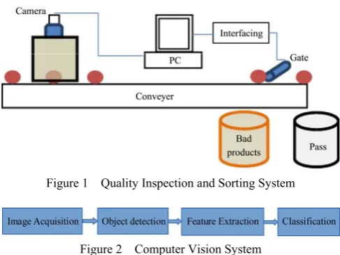
The vision-based quality inspection system consists of different sub-systems. Figure 1 shows the various components of the system. Fast single camera or multiple cameras are used to capture the image of the products. Single-camera with mirrors can be used to check the different sides of the product, while various cameras fixed in different directions get more precise images.
Usually, an isolated box with lighting is used to overcome lighting variation problems and get better pictures. The captured images are sent to the computer to be processed and analyzed in real-time. The decision, “pass” or “fail” is sent as an electronic signal to interfacing circuits. These circuits drive an automatic valve to open or close the path of the products. By closing the way, the product pushed to “bad product” store. Finally, high-quality products only will continue to the “pass” store. Sometimes, products classified into more than two classes. The different classes represent different degrees of quality.
Figure 1 Quality Inspection and Sorting System
Figure 2 Computer Vision System
The vision system consists of many modules, and it is required to finish all processing in real-time. Figure 2 shows the different modules of computer vision for food products sorting. The image acquisition module captures an image and stores the image in computer memory. The size and format of the image affect the speed and accuracy of the sorting system. High-resolution images contain many details of the product but require extended time for processing and classification. A low-resolution image is processed very fast, but the accuracy of the system can reduce. The suitable resolution should be chosen, give acceptable speed with the best efficiency.
classification. Another image segmentation is required to extract these regions (cracks- holes – different colors) from the product area. Features are extracted from product regions. The final step is a trained classifier, which gives the decision. The next sections present the data set, feature extraction, and classification.
3 Data set
The Food Cast Research Image Database (FRID) is an attempt at standardizing food-related objects (bakery products such as biscuits, fruits, edible nuts, vegetables, leafy vegetables, and food grains) dataset. In the dataset, all images size (530 ×530 pixels) are standardized and
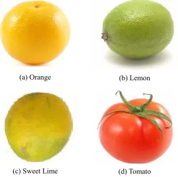
stored as .jpg file format. In this study, we have considered 1200 food-related images and categorized into a lemon (300 images), Orange (300 images), Sweet Lime (300 images), and Tomato (300 images). The sample dataset is shown in Figure 3.
(a) Orange (b) Lemon
(c) Sweet Lime (d) Tomato
Figure 3 Sample dataset
4 Feature extraction
The feature extraction is a significant phase in this research. We have used the segmented images of a different category from the FRID dataset. Then we have developed a feature extraction method to extract the features as Morphological, Color, and Texture. The HLS color space is used to remove the color characteristics of a categorized food product to measure luminance and chrominance. The measured color features are as follows (Sun, 2008):
i. Luminance (L): It describes the “achromatic” component, but generally represents the brightness of an image.
ii. Chrominance (C): The color information of an image and it is usually expressed as two color-difference components.
iii. Hue (H): It represents the dominant color.
iv. Color Distance Metric (ΔE): It is a metric of difference between colors.
The brightness and contrast of each color component are determined statistically as follows.
v. Mean (μ): The overall average intensity of each color component of an image.
vi. Standard Deviation (σ): The average distance from the mean of the total perceived brightness and contrast of each color component in an image.
vii. Range (r): The range of maximum and minimum perceived brightness of each color component in an image.
4.1 HSL Color space
There are two main aspects to rely on the importance of HSL color space: firstly, the chrominance components are hue and saturation, which separated from luminosity, and secondly, how much color spectrum human perceived given by these chrominance components (Plantations et al., 2000; Weijer and Schmid, 2006). The high color values for colors assigned in this space, which are approaching the white color with a bounded saturation. In this color space, color purity measured by hue (H), the degree of white color embedded in particular intensity measured by saturation (S) and the brightness of color measured by lightness (L).
The following steps are illustrating the conversion of RGB to HSL color space
Chroma calculation:
The R, G, and B values are divided by 255 to change the range from 0… 255 to 0,…., 1:
1 1 ( , ) / 255
r c
k l
R′ =
∑ ∑
= = R k l (1)1 1 ( , ) / 255
r c
k l
G′ =
∑ ∑
= =G k l(2)
1 1 ( , ) / 255
r c
k l
B′ =
∑ ∑
= = B k l (3)The Sun (2008) is given chroma definition as “colorfulness relative to the brightness of a similarly illuminated white.”
CHSL=Cmax–Cmin (4)
Hue calculation:
Sun (2008) is given hue definition as “attribute of a visual sensation according to which an area appears to be similar to one of the perceived colors: red, yellow, green, and blue, or to a combination of two of them.”
max
max
max
60 mod 6 ,
60 2 ,
60 4 ,
HSL HSL HSL HSL G B C R C B R
H C G
C R G C B C ′ ′ ⎧ ° ∗⎛ − ⎞ = ′ ⎪ ⎜⎝ ⎟⎠ ⎪ ⎪ ⎛ ′− ′ ⎞ ⎪ ′ =⎨ ° ∗⎜ + ⎟ = ⎝ ⎠ ⎪ ⎪ ⎛ ′− ′ ⎞ ′ ⎪ °∗⎜ + ⎟ = ⎪ ⎝ ⎠ ⎩
o (5)
Lightness or Luminosity calculation:
LHSL=(Cmax+Cmin)/2 (6)
Saturation calculation:
The ratio of colorfulness to brightness or of chroma to lightness is saturation.
0, 0
, 0
1 | 2 1|
HSL HSL HSL HSL HSL C S C C L = ⎧ ⎪ = ⎨ ≠ ⎪ − − ⎩ (7)
The mean, standard deviation, and range of each color components of Hue, Luminosity, and Saturation are determined.
(i) The mean, standard deviation, and range of hue component are determined using the following Equations (8), (9) and (10).
1 1
1
( , )
H
r c
HSL k l HSL
μ H k l
r c = =
=
∗
∑ ∑
o (8)
2 1 1 1 ( ( , ) ) H H r c
HSL k l HSL HSL
σ H k l μ
r c = =
= −
∗
∑ ∑
o (9)
1 1
1 1
max( ( , ))
min( ( , ))
H
r c
HSL k l HSL
r c
HSL
k l
r H k l
H k l
= =
= =
=
∑ ∑
−∑ ∑
o
o (10)
(ii) The mean, standard deviation, and range of Luminosity component are determined using the following Equations (11), (12) and (13).
1 1
1
( , )
L
r c
HSL k l
μ L k l
r c = =
=
∗
∑ ∑
(11)2 1 1 1 ( ( , ) ) L L r c
HSL k l HSL
σ L k l μ
r c = =
= −
∗
∑ ∑
(12)1 1 1 1
max( ( , )) min( ( , ))
L
r c r c
HSL k l k l
r =
∑ ∑
= = L k l −∑ ∑
= = L k l(13) (iii) The mean, standard deviation, and range of saturation component are determined using the following Equations (14), (15) and (16).
1 1
1
( , )
S
r c
HSL k l HSL
μ S k l
r c = =
=
∗
∑ ∑
(14)2 1 1 1 ( ( , ) ) S S r c
HSL k l HSL HSL
σ S k l μ
r c = =
= −
∗
∑ ∑
(15)1 1 1 1
max( ( , )) min( ( , ))
S
r c r c
HSL k l HSL k l HSL
r =
∑ ∑
= =S k l −∑ ∑
= =S k l(16) The color distance metric is calculated separately of Hue, Saturation, and Luminosity by using Equations (17), (18), and (19). And all three combined color distance metric is computed using Equation (20).
2
1 1
Δ H ( H ( , ))
r c
HSL k l HSL HSL
E =
∑ ∑
= = μ −Ho k l (17)2
1 1
Δ S ( S ( , ))
r c
HSL k l HSL HSL
E =
∑ ∑
= = μ −S k l (18)2
1 1
Δ L ( L ( , ))
r c
HSL k l HSL
E =
∑ ∑
= = μ −L k l (19)2 2 1 1 2 Δ ((( ( , )) (( ( , )) (( ( , )) ) H L S HSL r c
HSL HSL HSL
k l
HSL HSL
E
μ H k l μ L k l
μ S k l
= =
=
− + −
+ −
∑ ∑
o(20) We have the extracted 14 features from each sample, which listed in Table 1.
Table 1 The total extracted color measurement of HSL color space from each sample
Number Measurement Code
1 Mean of hue component μHSLH
2 Mean of saturation component μHSLS
3 Mean of the luminance component μHSLL
4 The standard deviation of the hue component σHSLH
5 The standard deviation of the saturation component σHSLS
6 Standard deviation of luminance component σHSLL
7 Range of hue component rHSLH
8 Range of saturation component rHSLS
9 Range of luminance component rHSLL
10 Chroma of HSL CHSL
11 Color distance metric of hue component ΔEHSLH
12 Color distance metric of saturation component ΔEHSLS
13 Color distance metric of luminance component ΔEHSLL
14 Color distance metric of HSL ΔEHSL
4.2 Gray level co-occurrence matrix method
a frequency matrix between sequential pixels in the image. The co-occurrence probabilities used for generating texture features. The co-occurrence probabilities used for making texture features. The co-occurrence probability is calculated by;
Pr(x)={P(i, j)|(d,Ɵ)} (21)
, 1
( , ) ij
G ij i j
P P i j
P
=
=
∑
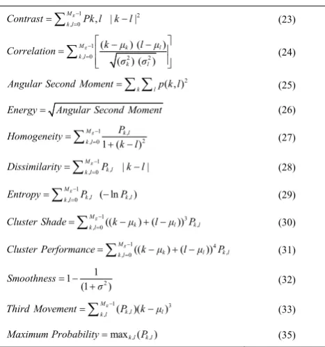
(22) Where, Pr(x) is the measure of the probability; P(i, j) is the co-occurrence probability between grey levels of i andj, and Pij is a number of the occurrence of the grey levels (Clausi, 2002). After calculating GLCM, texture features are obtained based on this co-occurrence matrix. There are 12 texture features (Haralick R. M., 1979) are calculated. Table 2 shows the GLCM features computed in this study.
Table 2 GLCM texture features (Haralick, 1979)
1 2
, 0 , | |
g
M k l
Contrast=∑ =−Pk l k l− (23)
1
, 0 2 2
( ) ( ) ( ) ( )
g
M k l
k l
k l
k μ l μ
Correlation σ σ − = ⎡ − − ⎤ ⎢ ⎥ = ⎢ ⎥ ⎣ ⎦ ∑ (24) 2
k l ( , )
Angular Second Moment=∑ ∑ p k l (25)
Energy= Angular Second Moment (26)
1 ,
2
, 01 ( )
g
M k l
k l P Homogeneity k l − = = + − ∑ (27) 1 ,
, 0 | |
g
M k l k l
Dissimilarity=∑ =−P k l− (28)
1
, ,
, 0 ( ln )
g
M
k l k l
k l
Entropy=∑ =−P − P (29)
1 3
, , 0
((Mg ) ( ))
k l k l
k l
Cluster Shade=∑ =− k−μ + −l μ P (30)
1 4
, , 0
((Mg ) ( ))
k l k l
k l
Cluster Performance=∑ =− k−μ + −l μ P (31)
2 1 1 (1 ) Smoothness σ = − + (32) 1 3 , , ( )( ) g M
k l l
k l
Third Movement=∑ − P k−μ (33)
, ,
max (k l k l)
Maximum Probability= P (35)
In this study, the GLCM-based texture features calculated for each sample. Extraction of color texture features conducted by computing the textural features for HSL color components. To represent a given image sample with a feature vector, 12 GLCM features are calculated for each color component. In this way, each image is represented with 14+(12 × 3)=50 features. Before applying any machine learning process, each feature is normalized to eliminate the drawback of significant differences between feature magnitudes. The normalization is performed between 0 and 1.
4.3 Feature selection and feature model
An optimum feature model defined as a subset of relevant features which best represents the data. In this study, the optimized set of a feature model is composed using principal component analysis (PCA). Which is a statistical procedure implementing orthogonal transformation to convert a set of samples of possibly correlated features into a set of values of linearly uncorrelated features called principal components (PCs) or eigenvectors? This method also determines a new feature space in which the data efficiently represented. The common way of obtaining relevant features is using only the first three principal components which represent most of the variability in the data (Kurtulmus and Ünal, 2015). Therefore, the first three PCs used as the second feature set for classifying category as Lemon, Orange, Sweet Lime, and Tomato.
4.4 Soft Computing Techniques
In pattern classification tasks, an optimum classifier depends on the nature of the data, and its ability to interpret interactions between the features. As a general approach, performances of the different classifiers can be tested by turning their specific parameters. In this study, different Soft computing techniques (Backpropagation neural network and Probabilistic Neural Network) and are also performed to find an optimal classification model.
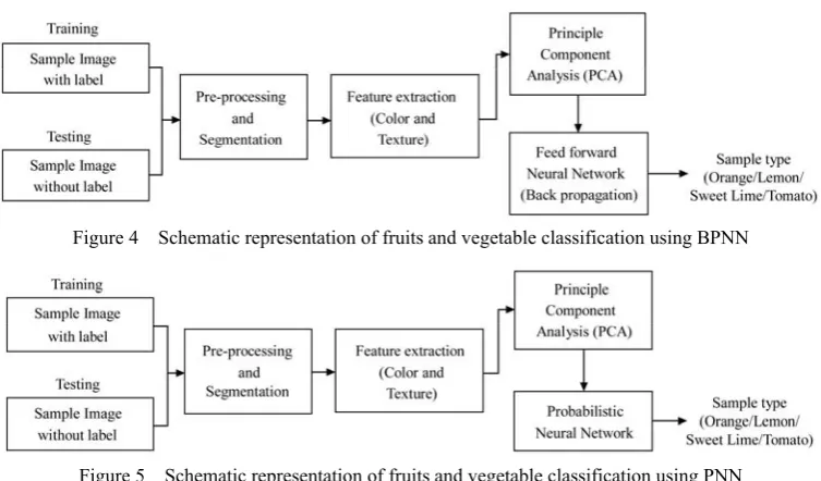
Multilayer feed-forward neural networks using backpropagation learning (Figure 4) and Probabilistic Neural Network (Figure 5) implemented for classification of four varieties; Lemon, Orange, Sweet Lime, and Tomato. For training, testing, and tuning the specific parameters of the classifiers, an approach based on the combination of 10-fold cross-validation method followed.
Learning rate is 0.9 throughout the momentum teaching rule. As an additional guard against over-fitting, the data sets divided into two randomly selected data sets; 50% of
data used for training, and 50% used for testing. The neural network toolbox of MATLAB 2016a software used for designing and testing of the BPNN model.
Figure 4 Schematic representation of fruits and vegetable classification using BPNN
Figure 5 Schematic representation of fruits and vegetable classification using PNN The Probabilistic Neural Network (PNN) based on
Bayes decision rule, and it uses Gaussian Parzen windows for estimating the probability density functions (pdf) required in Bayes rule. Next, needs a single spread value for pdf estimation which is proportional to Gaussian window width. Spread parameter or smoothing factor is comparable to the standard deviation of the Gaussian Parzen window. The excellent performance of PNN depends on the proper selection of the spread parameter. In this study, to develop PNN, we have considered the full features set to classify the four varieties such as Orange, Lemon, Sweet Lime, and Tomato. We have used the empirical spread parameter as a constant value (0.89) for training as well as test the features of the sample, which belongs to any one of the types, for classification. As an additional guard against over-fitting, the data sets are divided into two randomly selected data sets; 50% of data used for training, and 50% is used for testing. The neural network toolbox of MATLAB 2016a software used for designing and testing of the PNN model.
5 Results and discussion
The classification experiments are conducted on the color and texture features set. The 1200 total samples of which 300 images of Lemon, 300 images of Orange, 300 images of Sweet Lime, and 300 images of Tomato (from
each category: 150 samples as training and 150 samples as a test set), are chosen randomly. The 10-fold cross-validation is used for training and testing. For each fold, the proportion between the data used for training and data used for testing are 90%-10%. The investigation is to the identification of food products into a category namely Lemon, Orange, Sweet Lime, and Tomato. The obtained results of samples category are presented in Table 3.
Table 3 Classification results for sample category
BPNN PNN
Training Test Training Test Category
Accuracy in % Accuracy in % Accuracy in % Accuracy in %
Lemon 93.89 91.58 89.07 90.58 Orange 92.09 90.90 90.90 92.90 Sweet Lime 92.57 92.00 88.27 89.23
Tomato 94.03 90.00 92.43 93.80
For the training set, the obtained prediction accuracy using BPNN is for Lemon (93.89%), Orange (92.09%), Sweet Lime (92.57%) and Tomato (94.03%). For the test set, the obtained prediction accuracy is for Lemon (91.58%), Orange (90.90%), Sweet Lime (92.00%) and Tomato (90.00%).
(92.90%), Sweet Lime (89.23%) and Tomato (93.80%). The comparative analysis is made with earlier research work (Du and Sun, 2004), tabulated in Table 4. The test set accuracies are considered for comparative analysis.
Table 4 Comparative analysis with earlier research work
BPNN PNN
Category Feature Set Reported accuracy
%
Proposed accuracy
%
Reported accuracy
%
Proposed accuracy %
Lemon Color, Texture 90.45 91.58 --- 90.58 Orange Color 88.89 90.90 90.00 93.90 Sweet Lime Color, Texture 89.30 92.00 --- 89.00 Tomato Color, Texture 86.76 90.00 --- 93.80
It has observed the proposed methods outperformed compared to be reported in the literature.
6 Conclusion
Overall color and texture features were extracted from each sample image proved to be the precise method in recognizing categorized one. The study was limited to Lemon, Orange, Sweet Lime and Tomato; therefore further studies on more individual food products like fruits and vegetables are needed. The very high accuracy and prediction performance of the results helped us to develop food product quality evaluation and classification systems.
Acknowledgment
The authors are greatly indebted to the Department of Computer Science and Engineering. Manipal Institute of Technology-Manipal University, Manipal-India, for providing excellent lab facilities that make this work possible.
References
Brosa, T., and D. Sun. 2004. Improving quality inspection of food products by computer vision – a review. Journal of Food Engineering, 61(1): 3–16.
Burks, T. F., S. A. Shearer, and F. A. Payne. 2000. Classification of weed species using color texture features and discriminant analysis. Transactions of the American Society of Agricultural Engineers, 43(2): 441–448.
Chen, H., J. Wang, Q. Yuan, P. Wan. 2011. Quality classification of peanuts based on image processing. Journal of Food, Agriculture and Environment, 9(3-4): 205–209.
Chetima, M. M., and P. Payeur. 2012. Automated tuning of a vision-based inspection system for industrial food manufacturing. Instrumentation and Measurement Technology Conference (I2MTC), IEEE International.
Clausi, D. A. 2002. An analysis of co-occurrence texture statistics as a function of grey level quantization. Canadian Journal of Remote Sensing, 28(1): 45–62.
Du, C. J., and D. Sun. 2004. Recent developments in the applications of image processing techniques for food quality evaluation. Transaction of Food Science & Technology, 15(5): 230–249.
Kurtulmuş, F., and H. Ünal. 2015. Discriminating rapeseed varieties using computer vision and machine learning. Expert Systems with Applications: 1880–1891.
Hanbury A. 2002. The taming of the hue, saturation, and brightness color space. In CVWW’02-Computer Vision Winter Workshop,
234–243.
Haralick, R. M. 1979. Statistical and structural approaches to texture. Proceedings of the IEEE, 67(5): 786–804.
Jin, J., J. Li, G. Liao, X. Yu, and L. C. C. Viray. 2009. Methodology for potatoes defects detection with computer vision. In Proceedings of the International Symposium on Information Processing, 346–351. Huangshan, P.R. China, 21-23 August.
Plantaniotis, K. N., and A. N. Venetsanopoulas. 2000. Color Image Processing and Applications. Spinger-Verlag: 237–277. Kumar, M., and G. Bora, D. Lin. 2013. Image processing technique
to estimate geometric parameters and volume of selected dry beans. Journal of Food Measurement and Characterization,
7(2): 81–89.
Namias, R., C. Gallo, R. M. Craviotto, M. R. Arango, and P. M. Granitto. 2012. Automatic grading of green intensity in soybean seeds. In 13th Argentine Symposium on Artificial Intelligence, 96–104.
Narendra, V. G., and K. S. Hareesh. 2010. Quality inspection and grading of agricultural and food products by computer vision-a review. International Journal of Computer Applications, 2(1): 43–65.
Pydipati, R., T. F. Burks, and W. S. Lee. 2006. Identification of citrus disease using color texture features and discriminant analysis. Computers and Electronics in Agriculture, 52(1-2): 49–59.
Quispe, S. C., J. D. B. Tapia, M. N. L. Paredes, D. B. Aranibar, and P. Escarcina. 2013. Optimization of Brazil-nuts classification process through automation using colour spaces in computer vision. Journal of Computer Information Systems and Industrial Management Applications, 5: 623–630.
Soedibyo, D. W., U. Ahmad, K. B. Seminar, and D. M. Subrata. 2010. The development of automatic coffee sorting system based on image processing and artificial neural network. In
The International Conference on the quality information for competitive agricultural based production system and commerce, 272–275.
Sun, D. 2008. Computer vision technology for food quality evaluation. Food Science and Technology, International series: 57–80.
Velappan, C., G. Arivu, G. Prakash, A. Sada. S. Sarma, P. G. Student, and A. Grading. 2012. Online image capturing and processing using vision box hardware: Apple Grading.
International Journal of Modern Engineering Research, 2(3): 639–643.
Weijer, J. V. D., and C. Schmid. 2006. Coloring Local Feature Extraction. In 9th European Conference on Computer Vision:
334–348.
White, D. J., C. Svellingen, and N. J. C. Strachan. 2006. Automated measurement of species and length of fish by computer vision. Fisheries Research, 80(2-3): 203–210. Yeh, J. C. H., L. G. C. Hamey, T. Westcott, and S. K. Y. Sung.