The Canadian Earth System Model version 5 (CanESM5.0.3)

(1)

Geosci. Model Dev., 12, 4823–4873, 2019 https://doi.org/10.5194/gmd-12-4823-2019 © Author(s) 2019. This work is distributed under the Creative Commons Attribution 4.0 License.

The Canadian Earth System Model version 5 (CanESM5.0.3)

Neil C. Swart1,3, Jason N. S. Cole1, Viatcheslav V. Kharin1, Mike Lazare1, John F. Scinocca1, Nathan P. Gillett1, James Anstey1, Vivek Arora1, James R. Christian1,2, Sarah Hanna1, Yanjun Jiao1, Warren G. Lee1, Fouad Majaess1, Oleg A. Saenko1, Christian Seiler4, Clint Seinen1, Andrew Shao3, Michael Sigmond1, Larry Solheim1, Knut von Salzen1,3, Duo Yang1, and Barbara Winter1

1_{Canadian Centre for Climate Modelling and Analysis, Environment and Climate Change Canada, Victoria,} BC, V8W 2P2, Canada

2_{Fisheries and Oceans Canada, Institute of Ocean Sciences, Sidney, BC, Canada} 3_{University of Victoria, 3800 Finnerty Rd, Victoria, BC, V8P 5C2, Canada}

4_{Climate Processes Section, Environment and Climate Change Canada, Victoria, BC, V8P 5C2, Canada} Correspondence:Neil C. Swart (neil.swart@canada.ca)

Received: 22 June 2019 – Discussion started: 23 July 2019

Revised: 21 September 2019 – Accepted: 25 September 2019 – Published: 25 November 2019

Abstract. The Canadian Earth System Model version 5 (CanESM5) is a global model developed to simulate his-torical climate change and variability, to make centennial-scale projections of future climate, and to produce initialized seasonal and decadal predictions. This paper describes the model components and their coupling, as well as various as-pects of model development, including tuning, optimization, and a reproducibility strategy. We also document the stabil-ity of the model using a long control simulation, quantify the model’s ability to reproduce large-scale features of the his-torical climate, and evaluate the response of the model to ex-ternal forcing. CanESM5 is comprised of three-dimensional atmosphere (T63 spectral resolution equivalent roughly to 2.8◦) and ocean (nominally 1◦) general circulation models, a sea-ice model, a land surface scheme, and explicit land and ocean carbon cycle models. The model features relatively coarse resolution and high throughput, which facilitates the production of large ensembles. CanESM5 has a notably higher equilibrium climate sensitivity (5.6 K) than its prede-cessor, CanESM2 (3.7 K), which we briefly discuss, along with simulated changes over the historical period. CanESM5 simulations contribute to the Coupled Model Intercompari-son Project phase 6 (CMIP6) and will be employed for cli-mate science and service applications in Canada.

1 Introduction

A multitude of evidence shows that human influence is driv-ing acceleratdriv-ing changes in the climate system, which are un-precedented in millennia (IPCC, 2013). As the impacts of climate change are increasingly being felt, so is the urgency to take action based on reliable scientific information (UN-FCCC, 2015). To this end, the Canadian Centre for Climate Modelling and Analysis (CCCma) is engaged in an ongo-ing effort to improve modellongo-ing of the global Earth system, with the aim of enhancing our understanding of climate sys-tem function, variability, and historical changes, and making improved quantitative predictions and projections of future climate. The global coupled model, the Canadian Earth Sys-tem Model (CanESM), forms the basis of the CCCma mod-elling system and shares components with the Canadian Re-gional Climate Model (CanRCM) for finer-scale modelling of the atmosphere (Scinocca et al., 2016), the Canadian Mid-dle Atmosphere Model (CMAM) with atmospheric chem-istry (Scinocca et al., 2008), and the Canadian Seasonal to Interseasonal Prediction System which is used for seasonal prediction and decadal forecasts (CanSIPS, Merryfield et al., 2013).

(2)

4824 N. C. Swart et al.: CanESM5.0.3

1984; McFarlane et al., 1992). Successive versions of the model introduced a dynamic three-dimensional ocean in CGCM1 (Flato et al., 2000; Boer et al., 2000a, b), and later an interactive carbon cycle was included to form CanESM1 (Arora et al., 2009; Christian et al., 2010). The last major iteration of the model, CanESM2 (Arora et al., 2011), was used in the Coupled Model Intercomparison Project phase 5 (CMIP5) and continues to be employed for novel science applications such as generating large initial condition ensem-bles for detection and attribution (e.g. Kirchmeier-Young et al., 2017; Swart et al., 2018).

As detailed below, CanESM5 represents a major update to CanESM2. The leap from version 2 to version 5 was a one-off correction made to reconcile our internal model ver-sion labelling with the verver-sion label released to the public. The update includes incremental improvements to the atmo-sphere, land surface, and terrestrial ecosystem models. The major changes relative to CanESM2 are the implementa-tion of completely new models for the ocean, sea ice, and marine ecosystems, and a new coupler. Model developers have a choice in distributing increasing, but finite, computa-tional resources between improvements in model resolution, model complexity, and model throughput (i.e. number of years simulated). The resolution of CanESM5 (T63 or∼2.8◦ in the atmosphere and∼1◦in the ocean) remains similar to CanESM2 and is at the lower end of the spectrum of CMIP6 models. The advantage of this coarse resolution is a relatively high model throughput given the complexity of the model, which enables many years of simulation to be achieved with available computational resources. The first major applica-tion of CanESM5 is CMIP6 (Eyring et al., 2016), and over 50 000 years of simulation are being conducted for the 20 CMIP6-endorsed model intercomparison projects (MIPs) in which CCCma is participating.

The aim of this paper is to provide a comprehensive refer-ence that documents CanESM5. In the sections below, each of the model components is briefly described, and we also explain the approach used to develop, tune, and numerically optimize the model. Following that, we document the stabil-ity of the model in a long pre-industrial control simulation, and the model’s ability to reproduce large-scale features of the climate system. Finally, we investigate the sensitivity of the model to external forcings.

2 Component models

In CanESM5, the atmosphere is represented by the Cana-dian Atmosphere Model (CanAM5), which incorporates the Canadian Land Surface Scheme (CLASS) and the Canadian Terrestrial Ecosystem Model (CTEM). The ocean is rep-resented by a CCCma-customized version of the Nucleus for European Modelling of the Ocean model (NEMO), with ocean biogeochemistry represented by either the Canadian Model of Ocean Carbon (CMOC) in the standard model

ver-sion labelled as CanESM5, or the Canadian Ocean Ecosys-tem model (CanOE) in versions labelled CanESM5-CanOE. The atmosphere and ocean components are coupled by means of the Canadian Coupler (CanCPL). Each of these components of CanESM5 are described further below. 2.1 The Canadian Atmospheric Model version 5

(CanAM5)

Version 5 of the Canadian Atmospheric Model (CanAM5) employs a spectral dynamical core with a hybrid sigma-pressure coordinate in the vertical. The package of physi-cal parameterizations used by CanAM5 is based on an up-dated version of its predecessor, CanAM4 (von Salzen et al., 2013). The physics package includes a prognostic cloud microphysics scheme governing water vapour, cloud liquid water, and cloud ice; a statistical layer-cloud scheme; and independent cloud-base mass-flux schemes for both deep and shallow convection. Aerosols are parameterized using a prognostic scheme for bulk concentrations of natural and anthropogenic aerosols, including sulfate, black and organic carbon, sea salt, and mineral dust; parameterizations for emissions, transport, gas-phase and aqueous-phase chem-istry; and dry and wet deposition account for interactions with simulated meteorology. CanAM5 employs a triangular truncation at total wavenumber 63 (T63) corresponding to an approximate isotropic resolution of 2.8◦in both latitude and longitude. In the vertical, 49 levels are employed with layer thicknesses that increase monotonically from approximately 100 m at the surface to 2 km at∼1 hPa – the domain lid.

Updates to the package of physical parameterizations in CanAM5 over those in CanAM4 are as follows. While the radiative transfer solution in CanAM5 is similar to that in CanAM4, the representation of optical properties was im-proved through changes to the parameterization of albedos for bare soil, snow, and ocean whitecaps; cloud optics for ice clouds and polluted liquid clouds; improved aerosol op-tical properties and absorption by the water vapour contin-uum at solar wavelengths. For aerosols, the parameterization for emissions of mineral dust and dimethyl sulfide (DMS) was improved, while the bulk stratiform cloud microphysical scheme was modified to include a parameterization of the second indirect effect.

(3)

N. C. Swart et al.: CanESM5.0.3 4825

component. A full description CanAM5 and its relation to CanAM4 will be provided in a companion paper in this spe-cial issue (Cole et al., 2019).

2.2 CLASS-CTEM

The CLASS-CTEM modelling framework consists of the Canadian Land Surface Scheme (CLASS) and the Canadian Terrestrial Ecosystem Model (CTEM) which together form the land component of CanESM5. CLASS and CTEM simu-late the physical and biogeochemical land surface processes, respectively, and together they calculate fluxes of energy, wa-ter, CO2, and wetland CH4emissions at the land–atmosphere boundary. The introduction of dynamic wetlands and their methane emissions is a new biogeochemical process added since the CanESM2 (but note that these methane emissions are strictly diagnostic, since atmospheric methane concentra-tions are specified).

CLASS is described in detail in Verseghy (1991, 2000) and Verseghy et al. (1993) and version 3.6.2 is used in CanESM5. It prognostically calculates the temperature for its soil layers, their liquid and frozen moisture contents, temperature of a single vegetation canopy layer if it is present as dictated by the specified land cover, and the snow water equivalent and temperature of a single snow layer if it is present. Three per-meable soil layers are used with default thicknesses of 0.1, 0.25, and 3.75 m. The depth to bedrock is specified on the basis of the global dataset of Zobler (1986), which reduces the thicknesses of the permeable soil layers. CLASS per-forms energy and water balance calculations and all physical land surface processes for four plant functional types (PFTs) (needleleaf trees, broadleaf trees, crops, and grasses) and op-erates at the same subdaily time step as the rest of the atmo-spheric component.

CTEM models photosynthesis, autotrophic respiration from its three living vegetation components (leaves, stem, and roots), and heterotrophic respiration fluxes from its two dead carbon components (litter and soil carbon) and is described in detail in Arora (2003) and Arora and Boer (2003, 2005). CTEM’s photosynthesis module operates within CLASS, at the same time step as rest of the atmo-spheric component. CTEM provides CLASS with dynami-cally simulated structural attributes of vegetation including leaf area index (LAI), vegetation height, rooting depth and distribution, and aboveground canopy mass, which change in response to changes in climate and atmospheric CO2 concen-tration. All terrestrial ecosystem processes other than photo-synthesis are modelled in CTEM at a daily time step. Ter-restrial ecosystem processes in CTEM are modelled for nine PFTs that map directly to the PFTs used by CLASS. Needle-leaf trees are divided into their deciduous and evergreen types, broadleaf trees are divided into cold and drought de-ciduous and evergreen types, and crops and grasses are di-vided into C3and C4versions based on their photosynthetic pathways. The reason for separation of PFTs for CTEM is the

additional distinction that biogeochemical processes require. For example, the distinction between deciduous and ever-green versions of needleleaf trees is needed to simulate leaf phenology prognostically. Once leaf area index has been dy-namically determined by CTEM, all CLASS needs to know is that this PFT is a needleleaf tree since the physics calcula-tions do not require information about underlying deciduous or evergreen nature of leaves. Similarly, the C3and C4 photo-synthetic pathways of crops and grasses determine how they photosynthesize, thus affecting the calculated canopy resis-tance. However, once canopy resistance is known, CLASS does not need to know the underlying distinction between C3 and C4crops and grasses to use this canopy resistance in its energy and water balance calculations.

While the modelled structural vegetation attributes re-spond to changes in climate and atmospheric CO2 concentra-tion, the fractional coverage of CTEM’s nine PFTs is spec-ified. A land cover dataset is generated based on a potential vegetation cover for 1850 upon which the 1850 crop cover is superimposed. From 1850 onwards, as the fractional area of C3and C4crops changes, the fractional coverage of the other non-crop PFTs is adjusted linearly in proportion to their ex-isting coverage, as described in Arora and Boer (2010). The increase in crop area over the historical period is based on LUH2 v2h product (http://luh.umd.edu/data.shtml, last ac-cess: 1 October 2017) of the land use harmonization (LUH) effort produced for CMIP6 (Hurtt et al., 2011).

Both CanESM5 and its predecessor CanESM2 do not in-clude nutrient limitation of photosynthesis on land since the terrestrial nitrogen cycle is not represented. However, both models include a representation of terrestrial photosynthe-sis downregulation based on Arora et al. (2009), who used results from plants grown in ambient and elevated CO2 envi-ronments to emulate the effect of nutrient constraints. The tunable parameter determining the strength of this down-regulation, and therefore the strength of the CO2 fertiliza-tion effect, is higher in CanESM5 than in CanESM2, result-ing in higher land carbon uptake in CanESM5. The tunresult-ing of this downregulation parameter value, used in CanESM5, is explained in Arora and Scinocca (2016) who evaluate several aspects of modelled historical carbon cycle against observation-based estimates. A land nitrogen cycle model for CTEM is currently being developed, which will make the photosynthesis downregulation parameterization obsolete in future versions of the model.

(4)

wetland-to-4826 N. C. Swart et al.: CanESM5.0.3

upland heterotrophic respiratory flux and the fact that some of the CH4flux is oxidized in the soil column before reaching the atmosphere.

Surface runoff and baseflow simulated by CLASS are routed through river networks. Major river basins are dis-cretized at the resolution of the model and river routing is performed at the model resolution using the variable veloc-ity river-routing scheme presented in Arora and Boer (1999). The delay in routing is caused by the time taken by runoff to travel over land in an assumed rectangular river channel and a groundwater component to which baseflow contributes. Streamflow (i.e. the routed runoff) contributes freshwater to the ocean grid cell where the land fraction of a CanAM grid cell first drops below 0.5 along the river network as the river approaches the ocean.

In CanESM5, glacier coverage is specified and static. Grid cells are specified as glaciers if the fraction of the grid cell covered by ice exceeds 40 %, based on the GLC2000 dataset (Bartholomé and Belward, 2005). The combination of this threshold and the model resolution results in glacier-covered cells predominantly representing the Antarctic and Greenland ice sheets, with a few glacier cells in the Hi-malayas, northern Canada, and Alaska. Snow can accumu-late on glaciers, and any additional snow above the thresh-old of 100 kg m−2of snow water equivalent is converted into ice, and an equivalent mass of freshwater is immediately in-serted into runoff – implicitly representing mass balance be-tween accumulation and calving. Snow and ice on glaciers can be melted, with the water exceeding a ponding limit in-serted into runoff. There is no explicit accounting for glacier mass balance or adjustment of glacier coverage. This repre-sents a potentially infinite global source or sink of freshwater in the coupled system, particularly in climates which are far from the state represented by GLC2000. However, in prac-tice, the timescales of our centennial-scale simulations are much shorter than the response times of ice sheet coverage, and any imbalances are small (Sect. 4).

2.3 NEMO modified for CanESM (CanNEMO) The ocean component is based on NEMO version 3.4.1 (Madec and the NEMO team, 2012). It is configured on the tripolar ORCA1 C grid with 45z-coordinate vertical levels, varying in thickness from∼6 m near the surface to∼250 m in the abyssal ocean. Bathymetry is represented with partial cells. The horizontal resolution is based on a 1◦ Mercator grid, varying with the cosine of latitude, with a refinement of the meridional grid spacing to 1/3◦_{near the Equator. The} adopted model settings include the linear free surface for-mulation (see Madec and the NEMO team, 2012, and refer-ences therein). Momentum and tracers are mixed vertically using a turbulent kinetic energy scheme based on the model of Gaspar et al. (1990), implemented into NEMO physics by Blanke and Delecluse (1993). The tidally driven mixing in the abyssal ocean is accounted for following Simmons et

al. (2004). Base values of vertical diffusivity and viscosity are 0.5×10−5 and 1.5×10−4m2s−1_{, respectively. A} pa-rameterization of double diffusive mixing (Merryfield et al., 1999) is also included. Lateral viscosity is parameterized by a horizontal Laplacian operator with an eddy viscosity co-efficient of 1.0×104m2s−1 in the tropics, decreasing with latitude as the grid spacing decreases. Tracers are advected using the total variance dissipation scheme (Zalesak, 1979). Lateral mixing of tracers (Redi, 1982) is parameterized by an isoneutral Laplacian operator with an eddy diffusivity co-efficient of 1.0×103m2s−1at the Equator, which decreases poleward with the cosine of latitude. The process of poten-tial energy extraction by baroclinic instability is represented with the Gent and McWilliams (1990) scheme using a spa-tially variable formulation for the mesoscale eddy transfer coefficient, as briefly described below.

Two modifications have been introduced to NEMO’s mesoscale and small-scale mixing physics. The first modi-fication is motivated by the observational evidence suggest-ing that away from the tropics the eddy scale decreases less rapidly than does the Rossby radius (e.g. Chelton et al., 2011). This is taken into consideration in the formulation for the eddy mixing length scale, which is used to com-pute the mesoscale eddy transfer coefficient for the Gent and McWilliams (1990) scheme (for details, see Saenko et al., 2018). The second modification is motivated by the ob-servationally based estimates suggesting that a fraction of the mesoscale eddy energy could get scattered into high-wavenumber internal waves, the breaking of which results in enhanced diapycnal mixing (e.g. Marshall and Naveira Garabato, 2008; Sheen et al., 2014). A simple way to rep-resent this process in an ocean general circulation model was proposed in Saenko et al. (2012). Here, we employ an up-dated version of their scheme which accounts better for the eddy-induced diapycnal mixing observed in the deep South-ern Ocean (e.g. Sheen et al., 2014).

CanESM5 uses the LIM2 sea-ice model (Fichefet and Morales Maqueda, 1997; Bouillon et al., 2009), which is run within the NEMO framework. Some details regarding the calculation of surface temperature over sea ice are described in the coupling section below.

2.4 Ocean biogeochemistry

(5)

biogeo-N. C. Swart et al.: CanESM5.0.3 4827

chemical models simulate ocean carbon chemistry and abi-otic chemical processes such as oxygen solubility identically, in accordance with the Ocean Model Intercomparison Project Biogeochemistry (OMIP-BGC) protocol (Orr et al., 2017). 2.4.1 Canadian Model of Ocean Carbon (CMOC) The Canadian Model of Ocean Carbon was developed for earlier versions of CanESM (Zahariev et al., 2008; Christian et al., 2010; Arora et al., 2011) and includes carbon chemistry and biology. The biological component is a simple nutrient– phytoplankton–zooplankton–detritus (NPZD) model, with fixed Redfield stoichiometry, and simple parameterizations of iron limitation, nitrogen fixation, and export flux of cal-cium carbonate. CMOC was migrated into the NEMO mod-elling system, and the following important modifications were made: (i) oxygen was added as a passive tracer with no feedback on biology; (ii) carbon chemistry routines were updated to conform to the OMIP-BGC protocol (Orr et al., 2017); (iii) additional passive tracers requested by OMIP were added, including natural and abiotic dissolved inorganic carbon (DIC) as well as the inert tracers (CFC11, CFC12, and SF6).

2.4.2 Canadian Ocean Ecosystem Model (CanOE) The Canadian Ocean Ecosystem Model (CanOE) is a new ocean biology model with a greater degree of complexity than CMOC and explicitly represents some processes that were highly parameterized in CMOC. CanOE has two size classes for each of phytoplankton, zooplankton, and detri-tus, with variable elemental (C/N/Fe) ratios in phytoplank-ton and fixed ratios for zooplankphytoplank-ton and detritus. Each detri-tus pool has its own distinct sinking rate. In addition, there is an explicit detrital CaCO3variable, with its own sinking rate. Iron is explicitly modelled, with a dissolved iron state variable, sources from aeolian deposition and reducing sed-iments, and irreversible scavenging from the dissolved pool. N2 fixation is parameterized similarly to CMOC with tem-perature and irradiance dependence and inhibition by dis-solved inorganic nitrogen but no explicit N2-fixer group. In addition, N2 fixation is iron-limited in CanOE. In CanOE, denitrification is modelled prognostically and occurs only where dissolved oxygen is<6 mmol m−3. Deposition of or-ganic carbon is instantaneously remineralized at the sea floor as in CMOC, and CaCO3deposited at the sea floor dissolves if the calcite is undersaturated (whereas in CMOC, the burial fraction is implicitly 100 %). Carbon chemistry and all abi-otic chemical processes such as oxygen solubility conform to the OMIP-BGC protocol (Orr et al., 2017) and are identi-cal in CanOE and CMOC, except that in CMOC the carbon chemistry solver is applied only in the surface layer (as there is no feedback from saturation state to other biogeochemi-cal processes in the subsurface layers). CanOE has roughly twice the computational expense of CMOC.

2.5 The Canadian Coupler (CanCPL)

CanCPL is a new coupler developed to facilitate communica-tion between CanAM and CanNEMO. CanCPL depends on Earth System Modeling Framework (ESMF) library routines for regridding, time advancement, and other miscellaneous infrastructure (Theurich et al., 2016; Collins et al., 2005; Hill et al., 2004). It was designed for the multiple programme multiple data (MPMD) execution mode, with communica-tion between the model components and the coupler via the Message Passing Interface (MPI).

The fields passed between the model components are sum-marized in Tables A1–A4. In general, CanNEMO passes in-stantaneous prognostic fields, which are remapped by Can-CPL and given to CanAM as lower boundary conditions. These prognostic fields (sea-surface temperature, sea-ice concentration, and mass of sea ice and snow) are held con-stant in CanAM over the course of the coupling cycle. Af-ter integrating forward for a coupling cycle, CanAM passes back fluxes, averaged over the coupling interval, which are remapped in CanCPL and passed on to NEMO as sur-face boundary conditions. An exception is the ocean sursur-face CO2 flux, which is computed in CanNEMO and passed to CanAM. CanAM and CanNEMO are run in parallel, and the timing of exchanges through the coupler is indicated schematically in Fig. A1.

All regridding in CanCPL is done using the ESMF first-order conservative regridding option (ESMF, 2018), ensuring that global integrals remain constant for all quantities passed between component models (but see an exception below). The remapping weightswij, for a particular source celliand destination cellj, are given bywij=fij×Asi/(Adj×Dj),

wherefij is the fraction of the source cellicontributing to the destination cellj,Asi andAdjare the areas of the source

and destination cells, andDjis the fraction of the destination cell that intersects the unmasked source grid (ESMF, 2018).

Within the NEMO coupling interface, the “conservative” coupling option is employed. This option dictates that net fluxes are passed over the combined ocean–ice cell, and the fluxes over only the ice-covered fraction of the cell are also supplied, in principle allowing net conservation, even if the distribution of ice has changed given the unavoid-able one coupling cycle lag encountered in parallel coupling mode. It was verified that the net heat fluxes passed from CanAM were identical to the net fluxes received by NEMO, to the level of machine precision. Conservation in the cou-pled model piControl run is discussed further in Sect. 4.

(6)

an alternative GTice can be evaluated in CanAM at every model time step, taking into account evolving surface albedo and atmospheric temperature (e.g. West et al., 2016). As im-plemented, when computing GTice, CanAM independently computes the conductive heat flux through sea ice, and there is no constraint that this flux, or GTice, is the same as that in LIM2. Conservation is maintained because the net heat flux between the atmosphere and sea ice is computed in CanAM and applied to LIM2, but different ice surface temperatures could result. Both approaches to computing surface fluxes were tested in CanESM5 and no major impacts on sea ice or the broader climate system relative to the default model were discovered. However, a significantly shorter coupling cycle of 1 h was required for convergence when fluxes were computed from the LIM2 GTicethat was passed through the coupler. The shorter coupling period was required to more physically resolve the response to diurnal variations in ra-diative and sensible heat fluxes from the atmosphere (see, for example, West et al., 2016). The evaluation of fluxes from GTice computed in CanAM, on the other hand, was stable for coupling periods ranging from 1 to 24 h, with no major changes in the mean climate or variability immedi-ately apparent. A final coupling cycle interval of 3 h was implemented for CanESM5 with the computation of fluxes based on the CanAM evaluation of GTice. These choices rep-resented improved robustness and a compromise between greater efficiency (i.e. longer coupling periods) and maxi-mum “realism”, which would be the 1 h coupling dictated by the length of the NEMO time step.

After a significant number of CMIP6 production simula-tions were complete, it was determined that while conser-vative remapping was desirable for heat and water fluxes, it introduced issues in the wind-stress field passed from CanAM to CanNEMO. Specifically, since CanAM is nomi-nally 3 times coarser than CanNEMO, conservative remap-ping resulted in constant wind-stress fields over several NEMO grid cells, followed by an abrupt change at the edge of the next CanAM cell. This blockiness in the wind stress results in a non-smooth first derivative, and the resulting peaked wind-stress curl results in unphysical features in, for example, the ocean vertical velocities. Changing regridding of only wind stresses to the more typical bilinear interpo-lation, instead of conservative remapping, largely alleviates this issue. Sensitivity tests indicate no major impact on gross climate change characteristics such as transient climate re-sponse or equilibrium climate sensitivity, or on general fea-tures of the surface climate. However, there is an impact on local ocean dynamics, which led to the decision to submit a “perturbed” physics member to CMIP6. Hence, simulations submitted to CMIP6 labelled as perturbed physics member 1 (“p1”) use conservative remapping for wind stress, while those labelled as “p2” use bilinear regridding (see Sect. 3.4). A comparison between p1 and p2 runs is provided in Ap-pendix E.

2.6 Treatment of greenhouse gases

CanESM5 represents radiative forcing from individual greenhouse gases (GHGs). Aside from CO2, the concentra-tions of all radiatively active gases are specified and tran-siently evolve. Of these, CH4, N2O, and families of chlo-rofluorocarbons (CFCs) are assumed to be well mixed, while O3 is specified as varying spatially – typically employ-ing that prescribed for CMIP6 (Checa-Garcia et al., 2018). CanAM5 offers two modes for modelling CO2 concentra-tions – as specified time-evolving concentraconcentra-tions or as a three-dimensional passive tracer driven by land–ocean sur-face emissions, prognostically derived through interactive coupling with biogeochemical carbon models in the land and ocean. For example, CanESM5 can be run with prognostic CO2in concert with specified anthropogenic fossil fuel emis-sions to simulate atmospheric CO2 concentration through the historical and future periods. Wetland methane emissions simulated by CLASS-CTEM, in contrast, are purely diagnos-tic. While these emissions respond to changes in climate and atmospheric CO2concentration (through changes in vegeta-tion productivity), they do not modify atmospheric CH4 con-centrations, which are specified.

3 Model development and deployment 3.1 Model tuning and spin up

Each of the CanESM5 component models (CanAM5, CLASS-CTEM, and CanNEMO) were initially developed in-dependently, driven by observations in stand-alone configu-rations – CanAM5 in present-day (2003–2008) Atmospheric Model Intercomparison Project (AMIP) mode and Can-NEMO in pre-industrial (PI) OMIP-like mode using CORE bulk formulae. In these configurations, free parameters were initially adjusted to reduce climatological biases assessed via a range of diagnostics. Further details of the CanAM5 tuning may be found in Cole et al. (2019). The component models were then brought together in a pre-industrial configuration (i.e. the piControl experiment), which was evaluated based on an array of diagnostics. Several thousand years of coupled simulation were run during the finalization of the model, and an approach was taken whereby AMIP simulations would be used to derive parameter adjustments in CanAM, which would then be applied to the coupled model.

(7)

in the open ocean, which induces an average global cooling of∼0.5 W m−2_{in the piControl simulation, and was not} in-cluded in the previous version, CanESM2.

This initial coupled-model cold bias was rectified by ad-justing free parameters in CanAM, CLASS, and LIM2 in order to achieve a piControl simulation with a global-mean screen temperature of around 13.7◦C (roughly the absolute value provided for 1850–1900 by the NASA-GISS, Berkeley Earth, and HadCRUT4 datasets) and a sea-ice volume within the spread of CMIP5 models, while maintaining a net top-of-atmosphere (TOA) radiative balance as close to 0 W m−2 as possible. The specific parameters adjusted were emissiv-ity of snow (from 1 to 0.97), snow grain size on sea ice, the drainage parameter controlling soil moisture, the LIM2 pa-rameter controlling the lead closure rate (from 2.0 to 3.0), and most significantly the accretion rate in cloud micro-physics. The accretion rate exerted the largest control, and sensitivity to this parameter is described more fully in a com-panion paper (Cole et al., 2019).

The consequence of the adjustments in CanAM5 was an increase in the present-day TOA forcing in AMIP mode from ∼1 to∼2.5 W m−2. Nonetheless, historical simulations of the coupled CanESM5 initialized from its equilibrated pi-Control show an increase in TOA forcing roughly matching the observed values of∼0.7–1.0 W m−2over the 2003–2008 period for which CanAM5 was tuned in AMIP mode. The difference in patterns of sea surface temperature (SST) and sea-ice concentrations between the coupled model and ob-servations is thought to be the cause of these differences in TOA balance between coupled and AMIP mode.

The final adjustment was to the carbon uptake over land so as to better match the observed value over the historical period, and achieved via the parameter which controls the strength of the CO2fertilization effect (Arora and Scinocca, 2016). No more extensive tuning of CanESM5 was taken. Critically, no tuning of climate sensitivity was under-taken – the transient and equilibrium climate sensitivity of CanESM5 are purely emergent properties. Once the tuned final configuration of CanESM5 was available, ocean po-tential temperature and salinity fields were initialized from World Ocean Atlas 2009, while CanAM, CLASS-CTEM, and CMOC were initialized from the restarts from earlier de-velopment runs. The model was spun up for over 1500 years prior to the launch of the official CMIP6 piControl simula-tion, which extends for a further 2000 years.

3.2 Code management, version control, and reproducibility

CanESM5 is the first version of the model to be publicly re-leased, and this code sharing has been facilitated by the adop-tion of a new version-control-based strategy for code man-agement. Additional goals of this new system are to adopt in-dustry standard software development practices, to improve

development efficiency, and to make all CanESM5 CMIP6 simulations fully repeatable.

To maintain modularity, the code is organized such that each model component has a dedicated git repository for the version control of its source code (Table 1). A dedicated super-repository tracks each of the components as git sub-modules. In this way, the super-repo. keeps track of which specific versions of each component combine together to form a functional version of CanESM. A commit of the CanESM super-repo., which is representable by an eight-character truncated SHA1 checksum, hence uniquely defines a version of the full CanESM source code. The model de-velopment process follows an industry standard workflow (Table B1). New model features are merged onto the de-velop_canesmbranch, which reflects the ongoing develop-ment of the model. Specific model versions, such as that used for CMIP6, are given tags and issued DOIs for ease of reference. We use an internal deployment of gitlab to host the model code and associated issue trackers, and we mirror the code to the public online code-hosting platform at https://gitlab.com/cccma/canesm (last access: 15 Novem-ber 2019).

A dedicated ecosystem of software is used to config-ure, compile, run, and analyse CanESM simulations on Environment and Climate Change Canada (ECCC)’s high-performance computer (HPC) (Table B2). Several measures are taken to ensure modularity and repeatability. The source code for each run is recursively cloned from gitlab and is fully self contained. A strict checking routine ensures that any code changes are committed to the version control sys-tem and any run-specific configuration changes are captured in a dedicated configuration repository. A database records the SHA1 checksums of the particular model version and configuration used for every run, and these are included in CMIP6 NetCDF output for traceability. Input files for model initialization and forcing are also tracked for reproducibility (Table B1).

(8)

Table 1.Code structure and repositories.

Repository Purpose

CanESM The top-level super-repository, which tracks specific versions of the component submodules listed below, to form a function version of the model; also contains a CONFIG directory with configuration files for the model

CanAM The source code for the spectral dynamics and physics of CanAM

CanDIAG Diagnostic source code for analysing CanAM output; this repository also contains various scripting used to run the model

CanNEMO The CCCma modified NEMO source code, along with additional utility scripting

CanCPL The coupler source code

CCCma_tools A collection of software tools for compiling, running, and diagnosing CanESM on ECCC’s high-performance computer

Figure 1.Schematic of CanESM5 optimization. See Sect. 3.3 and Appendix C for details.

3.3 Model optimization and benchmarking

The ECCC HPC system consists of the following compo-nents: a “backend” Cray XC40, with two 18-core Broad-well CPUs per node (for 36 cores per node), and roughly 800 nodes in total, connected to a multi-PB lustre file sys-tem used as scratch space. This machine is networked to a “frontend” Cray CS5000, with several PB of attached spin-ning disk. This whole compute arrangement is replicated in a separate hall for redundancy, effectively doubling the avail-able resources. Finally, a large tape-storage system (HPNLS) is available for archiving model results.

The initial implementation of a CanESM5 precursor on this new HPC occurred around 1 November 2017. The orig-inal workflow roughly followed that used for CanESM2 CMIP5 simulations. All CanESM5 components (atmosphere

CanAM, coupler CanCPL, and ocean CanNEMO) were orig-inally running at 64-bit precision. The atmospheric compo-nent CanAM was running on two 36-core compute nodes, the coupler was running on a separate node, and the ocean com-ponent was running on three nodes, resulting in six nodes in total. The initial throughput on the system, without queue time, was around 4.6 years of simulation per wall-clock day (ypd), or alternatively 0.02 simulation years per core day, when normalizing by the number of cores used.

(9)

change was in converting the 64-bit CanAM component to 32-bit numerics. Since the remaining two components, Can-CPL and CanNEMO, are still running at the 64-bit precision, the communication between CanAM and CanCPL required the promotion of a number of variables from 32-bit preci-sion to 64-bit and back. The 32-bit CanAM implementation required a number of modifications to maintain the numeri-cal stability of the code. Calculations in some subroutines, most notably in the radiation code, were promoted to the 64-bit accuracy. Conservation of some tracers, in particular CO2, was compromised at the 32-bit precision, and some additional code changes to conserve CO2and maintain car-bon budgets were implemented. Significant effort was also invested in optimizing compiler options used for NEMO to maximize efficiency, while the scalability of the NEMO code allowed sensibly increasing the node count to keep pace with the accelerated 32-bit version of CanAM.

In the final setup, the CanAM/CanCPL components are running on three shared compute nodes, and the ocean com-ponent CanNEMO is running on five nodes, resulting in eight nodes overall. The combined effect of the improvements listed in Table C1 resulted in more than tripling the origi-nal throughput to about 16 ypd (Fig. 1). Despite the increase in the total node count from six to eight, the efficiency of the model also improved roughly 3-fold, from 0.02 simulation years per core day of compute to about 0.06 years per core day. This final model configuration can complete a realiza-tion of the 165-year CMIP6 historical experiment in just over 10 d, compared to about 36 d, had no optimization been un-dertaken. At the time of writing, over 50 000 years of CMIP6 related simulation have been conducted with CanESM5, con-suming about 1 million core days of compute time, resulting in about 8 PB of data archived to tape and over 100 TB of data publicly served on the Earth System Grid Federation (ESGF).

3.4 Model experiments and scientific application This section describes the major experiments and model vari-ants of CanESM5 that are being conducted for the Coupled Model Intercomparison phase 6 (CMIP6), the first major sci-ence application of the model. Figure 2 shows the global-mean surface temperature for several of the key CMIP6 ex-periments, which can be used to infer important properties of the model, as discussed further in Sects. 4–6. Table 2 lists the variants of CanESM5 which are being submitted to CMIP6. These include the “p1” and “p2” perturbed physics members of CanESM5 (see Sect. 2.5) and a version of the model with a different ocean biogeochemistry model, CanESM5-CanOE.

Table D1 lists the 20 CMIP6-endorsed MIPs in which CanESM5 is participating and which model variants are be-ing run for each MIP. The volume of simulation continues to grow and will likely exceed 60 000 years. This is signif-icantly more than the∼40 000 years of CMIP6 simulation estimated by Eyring et al. (2016). The major reason for this

Figure 2. Global average screen temperature in CanESM5 for the CMIP6 DECK experiments, as well as the historical and tier 1 Shared Socioeconomic Pathway (SSP) experiments (SSP5-85, SSP3-70, SSP2-45, and SSP1-26). Thick lines are the 11-year run-ning means; thin lines are annual means.

is that significantly larger ensembles have been produced than formally requested. For example, CanESM5 will sub-mit at least 25 realizations for the historical and tier 1 Shared Socioeconomic Pathway (SSP) experiments for each of the “p1” and “p2” model variants, for a total of 50 realizations, significantly more than the single requested realization. The scientific value of such large initial condition ensembles has become evident (e.g. Kay et al., 2015; Kirchmeier-Young et al., 2017; Swart et al., 2018) and motivates this approach.

Individual historical realizations (ensemble members) of CanESM5 were generated by launching historical runs at 50-year intervals off the piControl simulation. This is the same as the approach used to generate the five realizations of CanESM2, which were submitted to CMIP5. The 50-year separation was chosen to allow for differences in multi-decadal ocean variability between realizations. Below, we discuss the properties of the model, including illustrations of the internal variability generated spread across the historical ensemble. All results below are based on the CanESM5 p1 model variant.

4 Stability of the pre-industrial control climate

(10)

long-4832 N. C. Swart et al.: CanESM5.0.3

Table 2.Model variants.

Model variant Description

CanESM5 “p1” CanESM5 realizations labelled as perturbed physics member 1 (“p1” in the variant label) have conservative remapping of wind-stress fields. The ocean biogeochemistry model is CMOC.

CanESM5 “p2” CanESM5 realizations labelled as perturbed physics member 2 (“p2” in the variant label) use bilinear remapping of the wind-stress fields. A minor land-fraction change also occurs over Antarctica. The ocean biogeochemistry model is CMOC.

CanESM5-CanOE “p2” CanESM5-CanOE is exactly the same physical model as CanESM5, but it uses the CanOE ocean biogeo-chemical model. All CanESM5-CanOE realizations use bilinear remapping of the wind stress and hence are labelled as perturbed physics member 2 (“p2” in the variant label). No “p1” variant is submitted. For physi-cal climate purposes, CanESM5 and CanESM5-CanOE are the same model, and simulations with specified CO2are bit identical in all realms besides ocean biogeochemistry. In runs with prognostic CO2(such as the esm-hist experiment), the physical climate of CanESM5 and CanESM5-CanOE will differ due to the effect of interactive CO2in these simulations.

term average, zero net fluxes of heat, freshwater, and car-bon at the interface between the atmosphere, ocean, and land surface, zero top-of-atmosphere net radiation, and constant long-term average temperatures or tracer mass within each component. In reality, however, models are not perfectly con-servative due to the limitations of numerical representation (i.e. machine precision) as well as possible design flaws or bugs in the code, and models are generally not run to perfect equilibrium due to computational constraints. Despite imper-fect conservation or spinup, models can still usefully be ap-plied, as long as the drifts in the control run are small relative to the signal of interest, in our case historical anthropogenic climate. Below, we consider conservation and drift of heat, water, and carbon in CanESM5 (Fig. 3).

The CanESM5 pre-industrial control shows a stable TOA net heat flux of 0.1 Wm−2(fluxes positive downward in m2 of global area; Fig. 3a). The model is close to radiative equi-librium and this control net TOA heat flux is over an or-der of magnitude smaller than the signal expected from his-torical anthropogenic forcing (>1 Wm−2). The global-mean screen temperature is stable at around 13.4◦C (Fig. 3d), in-dicating thermal equilibrium, and approximately in line with estimates of the temperature in 1850. Half of the net TOA flux is passed from the atmosphere to the ocean (0.05 Wm−2, Fig. 3b). With the conservative remapping in the coupler, the fluxes exchanged between components are identical to ma-chine precision. However, the net heat flux received at the surface of the liquid ocean is 0.14 Wm−2, almost 3 times higher than the heat flux passed from CanAM to NEMO (Fig. 3b). This discrepancy reflects a non-conservation of heat within the LIM2 ice model. Tests with an ice-free ocean do not suffer this problem. Nonetheless, the discrepancy is relatively small, and ice volume is stable. A further non-conservation occurs within the NEMO liquid ocean. Al-though the ocean receives a net heat flux of 0.14 Wm−2, the volume-averaged ocean is cooling at a rate equivalent to a flux of 0.05 Wm−2 (Fig. 3c), implying a total

non-conservation of heat in the liquid ocean of about 0.2 Wm−2. Conservation errors of this order are well known in NEMO v3.4.1, likely arise from the use of the linear free surface (Madec and the NEMO team, 2012), and have been seen in previous coupled models using NEMO (Hewitt et al., 2011). Despite this, the volume-averaged ocean temperature drift in CanESM5 is about half the size of the drift in CanESM2. Fur-thermore, the lack of ocean heat conservation in CanESM5 is roughly constant in time and appears to be independent of the climate (not shown).

At the liquid ocean surface, a small net freshwater flux re-sults in a freshening trend and sea-level rise of about 24 cm over 1000 years (Fig. 3e, f). This rate of drift is more than 20 times smaller than the signal of anthropogenic sea-level rise. The LIM2 ice model appears to be the source of non-conservation: the net freshwater flux provided from CanAM is very close to zero, about 6 times smaller than that noted above (24 cm per 1000 years). Snow and ice volume are stable, not exhibiting any long-term drift, yet they are sub-ject to considerable decadal- and centennial-scale variability (Fig. 3g, h).

(11)

Figure 3.Stability of the CanESM5 piControl run showing global-mean(a)top-of-atmosphere net heat flux,(b)net heat flux at the surface of ocean;(c)volume-averaged ocean temperature;(d)screen temperature;(e)net freshwater input at the liquid ocean surface;(f)dynamic sea level;(g)sea-ice volume;(h)snow mass;(i)land–atmosphere carbon flux;(j)ocean–atmosphere carbon flux;(k)terrestrial soil carbon mass; and(l)ocean-dissolved inorganic carbon concentration. Inset numbers are the time average over the 1000 years shown. Heat fluxes in panels(a)and(b)are reported per metre squared of global area. The orange line in panel(b)is the heat flux computed at the bottom of the atmosphere, while the grey line is the heat flux computed at the surface of the liquid ocean (below sea ice).

5 Evaluation of historical-mean climate

In this section, we use the CMIP6 historical simulations (Eyring et al., 2016) of CanESM5 “p1”, focusing on cli-matologies computed over 1981 to 2010, unless otherwise noted.

5.1 Overall skill measures

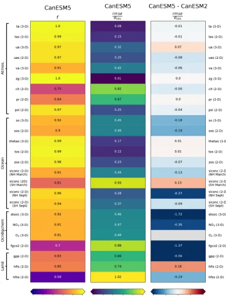
The ability of CanESM5 to reproduce observed large-scale spatial patterns in the climate system is quantified using global summary statistics computed over the 1981 to 2010 mean climate (Fig. 4). Shown are the correlation coeffi-cient between CanESM5 and observations (r), the root mean square error (RMSE) normalized by the observed (spa-tial) standard deviation (σ), and the change in normalized

RMSE between CanESM2 and CanESM5. The statistics are weighted by grid cell area for 2-D fields and volume for 3-D ocean fields, and by area and pressure for 3-D atmo-spheric variables. In general, CanESM5 successfully repro-duces many observed spatial patterns of the surface climate, interior ocean, and the atmosphere, with correlation coeffi-cients between the model and observations generally above 0.8. Some exceptions are the total cloud fraction (clt,r= 0.75), atmosphere–ocean CO2flux (fgco2,r=0.7), and the surface sensible heat flux (hfss,r=0.58).

(12)

(13)

Figure 5.Climatologies of surface air temperature over 1981 to 2010 in CanESM5(a, c)and their bias from ERA5 over the same period(b, d)

shown for the DJF(a, b)and JJA(c, d)seasons.

Figure 6.Climatologies of precipitation over 1981 to 2010 in CanESM5(a, c)and their bias from the Global Precipitation Climatology Project (GPCP) over the same period(b, d)shown for the DJF(a, b)and JJA(c, d)seasons.

winds (ua), sea-surface temperatures (tos), the March distri-bution of sea ice in the Southern Hemisphere (siconc), and surface latent heat flux (hfls). In the following sections, in-dividual realms are examined, with a closer look at regional details and biases.

5.2 Atmosphere

CanESM5 reproduces the large-scale climatological features of surface air temperatures (Fig. 5), precipitation (Fig. 6), and

(14)

Figure 7.Climatologies of sea-level pressure over 1981 to 2010 in CanESM5(a, c)and their bias from ERA5 over the same period(b, d)

shown for the DJF(a, b)and JJA(c, d)seasons.

Figure 8.Cloud fraction in CanESM5(a, c)and their bias with respect to International Satellite Cloud Climatology Project H series (ISCCP-H) satellite-based observations(b, d)shown for the DJF(a, b)and JJA(c, d)seasons.

North America, much of Siberia, and broad regions of the tropical and subtropical oceans.

Precipitation biases vary in sign by region (Fig. 6). The largest biases are over the tropical Pacific and Atlantic oceans, between the Equator and extending into the south-ern subtropics. The overall pattsouth-ern of precipitation biases is very similar to that seen across the CMIP5 (Flato et al., 2013) and CMIP3 (Lin, 2007) models. The largest land bi-ases are excessive precipitation over much of sub-Saharan Africa, southeast Asia, Canada, and Peru–Chile. In contrast,

western Asia, Europe, the North Atlantic, and the subtropi-cal to high-latitude Southern Ocean have too little simulated precipitation. The large-scale pattern of sea-level pressure is captured by CanESM5 (Fig. 7). Biases relative to ERA5 are largest over the high elevations of Antarctica (Fig. 7), possi-bly reflecting differences in the extrapolation of surface pres-sure to sea level.

(15)

east-N. C. Swart et al.: CanESM5.0.3 4837

Figure 9.Zonal-mean temperature in CanESM5(a, c)and bias relative to ERA5(b, d)over 1981–2010 for the DJF(a, b)and JJA(c, d)

seasons.

(16)

Figure 11. (a)Zonal surface winds in CanESM5, (b)the bias relative to ERA5, and(c)zonal-mean zonal surface winds in CanESM2, CanESM5, and ERA5.

ern tropical Pacific and Atlantic (Fig. 8). A too-large cloud fraction is also found over Antarctica and the Arctic. Under-estimations of total cloud fraction occur over most other land areas, with the largest underestimations over Asia and the Himalayas.

Zonal-mean sections of air temperature for the DJF and JJA seasonal means are shown in Fig. 9. In both sea-sons, CanESM5 is biased warm relative to ERA5 near the tropopause, across the tropics and subtropics. Warm biases also occur in the stratosphere, notably near 60◦S above

50 hPa in JJA. Cold biases exist from the subtropics to the high latitudes, where they reach from the surface to the stratosphere, and are strongest in the winter season.

(17)

Figure 12.Time-mean values of(a)gross primary productivity (GPP), (c)latent heat flux (hfls), and(e)sensible heat flux (hfss) from CanESM5 (r1i1p1f1)(a, c, e)and the corresponding biases with respect to observation-based reference data presented in Jung et al. (2009)

(b, d, f). Black dots mark grid cells where biases are not statistically significant at the 5 % level using the two-sample Wilcoxon test.

5.3 Land physics and biogeochemistry

Figures 12 and 13 compare the geographical distribution and zonal averages of gross primary productivity (GPP) and la-tent and sensible heat fluxes over land with observation-based estimates from Jung et al. (2009). The zonal averages of GPP, and latent and sensible heat fluxes compare reason-ably well with observation-based estimates, although the la-tent heat fluxes are somewhat higher especially in the South-ern Hemisphere, as discussed below (Fig. 13). Figure 12 shows the biases in the simulated geographical distribution of these quantities. In the tropics, biases in GPP, and latent and sensible heat fluxes broadly correspond to biases in sim-ulated precipitation compared to observation-based estimates (shown in Fig. 6).

Generally over the tropics, as would be intuitively ex-pected, the signs of GPP and latent heat flux anomalies are the same since they are both affected by precipitation in the same way. Sensible heat flux is expected to behave in the op-posite way compared to GPP and latent heat flux in response to precipitation biases. For example, simulated GPP and la-tent heat fluxes are lower, and sensible heat fluxes higher in

the northeastern Amazonian region because simulated pre-cipitation is biased low (Fig. 6). The opposite is true for al-most the entire African region south of the Sahara and al-most of Australia. Here, simulated precipitation that is biased high, compared to observations, results in simulated GPP and la-tent heat flux that are higher and sensible heat flux that is lower than observation-based estimates. At higher latitudes, where GPP and latent heat flux are limited by temperature and available energy, the biases in precipitation do not trans-late directly into biases in GPP and trans-latent heat flux as they do in the tropics.

(18)

re-4840 N. C. Swart et al.: CanESM5.0.3

Figure 13.Zonal-mean values of(a)GPP,(b)HFLS, and(c)HFSS for CanESM5 (r1i1p1f1) and reference data from Jung et al. (2009). The shading presents the corresponding interquartile range that results from interannual variability as well as longitudinal variability for the period 1982 to 2008.

duced evapotranspiration, some of which is recycled back into precipitation. Figure 14 shows the functional relation-ships between GPP and temperature, and GPP and precipi-tation, for both model- and observation-based estimates. The observation-based temperature and precipitation data used in these plots are from CRU-JRA reanalysis data that were used to drive terrestrial ecosystem models in the TRENDY inter-comparison for the 2018 Global Carbon Budget (Le Quéré et al., 2018). Figure 14 shows that GPP increases both with

(19)

Figure 14.Functional response of GPP to(a)near-surface air temperature and(b)surface precipitation for CanESM5 (r1i1p1f1) and refer-ence data from Jung et al. (2009). Values present monthly mean values averaged over the period 1982 to 2008 and the shading shows the corresponding standard deviation.

GPP relationship with precipitation compares much better to its observation-based relationship than that for temperature.

As mentioned earlier, dynamically simulated wetland ex-tent and wetland methane emissions in CanESM5 are purely diagnostic. Figure G1 in Appendix G compares zonal dis-tribution of simulated annual maximum wetland extent with observation-based estimates and shows the temporal evo-lution of annual maximum wetland extent and wetland methane emissions over the historical period.

5.4 Physical ocean

CanESM5 reproduces the observed large-scale features of sea-surface temperature (SST), salinity (SSS), and height (SSH) (Fig. 15). The largest SST biases are the cold anomalies southeast of Greenland and in the Labrador Sea (Fig. 15b). These negative SST biases are associated with excessive sea-ice cover, described further below, and with the surface air temperature biases mentioned above. Positive SST biases are largest in the eastern boundary current up-welling systems, as for surface air temperatures.

Sea-surface salinity biases are largest, and positive, around the Arctic coastline, potentially indicating insufficient runoff in this region (Fig. 15d). Negative annual-mean SSS biases occur in the Labrador Sea and are also found in seas of the maritime continent and eastern tropical Atlantic. SSH is shown as an anomaly from the (arbitrary) global mean (Fig. 15e). Significant SSH biases are associated with the positions of western boundary currents, noticeably for the Gulf Stream and Kuroshio Current (Fig. 15f). CanESM5 has too-low SSH around Antarctica and too-high SSH in the southern subtropics, with an excessive SSH gradient across the Southern Ocean. This SSH gradient is associated with the geostrophic flow of the Antarctic Circumpolar Current (ACC). The ACC in CanESM5 is vigorous with 190 Sv of transport through Drake Passage. This is larger than observa-tional estimates, which range up to 173.3±10.7 Sv (Dono-hue et al., 2016). In CanESM5, the ACC also exhibits a pro-nounced, centennial-scale variability of about 20 Sv, which is also evident in the piControl simulation (not shown).

(20)

Figure 15.Sea-surface(a)temperature,(c)salinity, and(e)height averaged over 1981 to 2010, their biases relative to World Ocean Atlas 2009(b, d), and the Aviso mean dynamic topography(f).

(21)

Figure 17.CanESM5 residual meridional overturning circulation in the Atlantic(a), Indo-Pacific(b), and global(c)oceans, averaged over 1981 to 2010, including all resolved and parameterized advective processes. Note that the depth scale on theyaxis is non-uniform.

(Fig. 4). In the zonal mean, potential temperature biases are largest within the thermocline, which is warmer than ob-served, particularly near 50◦_{N (Fig. 16a, b). The deep ocean,} the Southern Ocean south of 50◦S, and the Arctic Ocean are cooler than observed. The pattern of excessive heat accumu-lation in the thermocline is very similar to the pattern of bias seen in CMIP5 models on average (Flato et al., 2013, their Fig. 9.13). Also similar to CMIP5 models, there is a cold bias in the ocean below the thermocline. This suggests that the processes controlling the redistribution of heat between the thermocline and the deep ocean play a role in

(22)

Figure 18. Northward heat transport in the global ocean in CanESM5 (in petawatts), with error bars showing the inverse es-timate of Ganachaud and Wunsch (2003).

The meridional overturning circulation in the global ocean and the Indo-Pacific as well as Arctic–Atlantic basins is shown in Fig. 17. The global overturning streamfunction shows the expected major features: an upper cell with clock-wise rotation, connecting North Atlantic deep water forma-tion to low-latitude and Southern Ocean upwelling; a vigor-ous Deacon cell in the Southern Ocean (as a result of plot-ting inzcoordinates); a lower anticlockwise cell of Antarctic Bottom Water, and vigorous near-surface cells in the sub-tropics. The upper cell overturning rate at 26◦N in the At-lantic is estimated to be 17±4.4 Sv from the RAPID obser-vational array (McCarthy et al., 2015). CanESM5 produces an Atlantic overturning rate of 12.8 Sv at 26◦N, below the mean but within the range measured by RAPID. The fairly weak Atlantic meridional overturning circulation (AMOC) in CanESM5 is likely associated with excessive sea-ice cover in the Labrador Sea, which inhibits convection. However, we also note that NEMO models have previously been found to underestimate the AMOC (Danabasoglu et al., 2014).

Closely connected to the MOC is the rate of northward heat transport by the ocean (Fig. 18). CanESM5 produces the expected latitudinal distribution of heat transport but, consis-tent with a weak MOC, slightly underestimates the transport at 24◦N, relative to the inverse estimate of Ganachaud and Wunsch (2003). To the north and south, CanESM5 ocean heat transport falls within the observational uncertainties. The MOC and heat transport in CanESM5 are similar to those in CanESM2, as reported in Yang and Saenko (2012).

5.5 Sea ice

The seasonal cycles of sea-ice extent and volume are shown in Fig. 19. A major change from CanESM2 is seen in the sea-ice volume (Fig. 19b, d). CanESM2 simulated very thin sea-ice and had about 40 % less Northern Hemisphere (NH) ice vol-ume than in the Pan-Arctic Ice Ocean Modeling and Assim-ilation System (PIOMAS) reanalysis (Zhang and Rothrock, 2003; Schweiger et al., 2011). By contrast, CanESM5 has a larger NH ice volume than in CanESM2 (Fig. 19b). The amplitude and phase of the annual cycle in NH sea-ice vol-ume in CanESM5 are similar to those in PIOMAS (Fig. 19b). In the Southern Hemisphere, CanESM5 also has a larger sea-ice volume and a seasonal cycle far more consistent with the global PIOMAS (GIOMAS) reanalysis product than CanESM2 (Fig. 19d).

While CanESM2 significantly underestimated NH sea-ice extent relative to satellite-based observations, CanESM5 generally overestimates the extent (Fig. 19a). The NH sea-ice extent biases are largest in the winter and spring. During the March maximum, excessive sea ice is present in the Labrador Sea and east of Greenland (Fig. 20a). In the summer and fall, the net NH extent bias is far smaller (Fig. 20c) and results from a cancellation between lower-than-observed concen-trations over the Arctic basin and larger-than-observed con-centrations around northeastern Greenland. Southern Hemi-sphere sea-ice extent biases are largest during the early months of the year, and in March the positive concentration biases are focused in the northeastern Weddell and Ross seas (Fig. 20b). In September, SH concentration biases between CanESM5 and the satellite observations are focused around the northern ice edge and are of varying sign (Fig. 20d). 5.6 Ocean biogeochemistry

The standard configuration of CanESM5 has a significantly improved representation of the distribution of ocean bio-geochemical tracers relative to CanESM2, despite using the same biogeochemical model (CMOC). For the three-dimensional distributions of DIC and NO3, and the surface CO2flux, the RMSE, relative to observed distributions, was reduced by over a factor of 2 (Fig. 4). Ocean-only simula-tions, whereby NEMO was driven by CanESM2 surface forc-ing via bulk formulae, show similar skill to the CanESM5 coupled model. From this, we infer that changes in interior ocean circulation, rather than boundary forcing, are responsi-ble for the improved representation of biogeochemical tracer distributions.

(23)

Figure 19.Seasonal cycles of sea-ice extent(a, c)and volume(b, d)in the Northern Hemisphere(a, b)and Southern Hemisphere(c, d)

averaged over 1981 to 2010. Results are shown for CanESM2, CanESM5, the National Snow and Ice Data Center (NSIDC) satellite-based observations, and the PIOMAS and GIOMAS reanalyses.

(Fig. 21d). Elsewhere, zonal-mean NO3 concentrations are generally too low, particularly in the NH thermocline and the Arctic. CanESM5 has higher-than-observed concentrations of zonal-mean O2 (Fig. 21f). As expected from saturation, biases are largest in the Southern Ocean and abyssal ocean, where CanESM5 is colder than observed. However, positive O2biases also occur at the base of the thermocline in the NH, where CanESM5 is too warm, suggestive of a biological ori-gin.

The zonal-mean NO3biases identified at the thermocline level above are the result of partially cancelling biases be-tween the Pacific and Atlantic basins (not shown). The At-lantic has negative NO3biases, largest near 1000 m. Mean-while, there is an excessive accumulation of NO3centred at the base of the eastern Pacific thermocline. This buildup oc-curs due to the simplified parameterization of denitrification in CMOC. Within each vertical column, the amount of den-itrification is set to balance the rate of nitrogen fixation and is distributed vertically proportional to the detrital reminer-alization rate. In reality, nitrogen fixation and denitrification are not constrained to balance within the water column at any one location, but rather denitrification proceeds within anoxic areas. A prognostic implementation of denitrification implemented into CanOE resolves this bias and will be

dcussed further in an upcoming article within this special is-sue.

The atmosphere–ocean CO2flux pattern in CanESM5 cor-relates significantly better with estimates of the observed flux than that in CanESM2 (Fig. 4). The largest departures from the observations are positive biases in the southeastern Pa-cific, northwest PaPa-cific, and northwest Atlantic (Fig. 22b). These are compensated by negative biases in the Southern Ocean and midlatitude northeast Pacific. In the zonal mean, CanESM2 had a large flux dipole in the Southern Ocean, which is significantly reduced in CanESM5, and attributable to improved circulation in the new NEMO ocean model and a reduction in Southern Ocean wind speed biases in CanAM5 (Fig. 22c).

5.7 Modes of climate variability 5.7.1 El Niño–Southern Oscillation

(24)

Figure 20.Sea-ice concentration biases between CanESM5 and NSIDC climatologies for the months of March(a, c)and September(b, d)in the Northern Hemisphere(a, b)and Southern Hemisphere(c, d). The solid black contour marks the ice edge (15 % threshold) in CanESM5, and the teal line marks the ice edge in the observations. Biases are based on the 1981 to 2010 climatology.

first 10 historical ensemble members is compared against the Hadley Centre Sea Ice and Sea Surface Temperature (HadISST) dataset. The skill of CanESM5 at representing the local and remote effects of ENSO is evaluated by cor-relating SST anomalies with the resulting NINO3.4 index (Fig. 23a, b). Within the equatorial Pacific, a positive ENSO event in CanESM5 leads to an increase in SSTs across the en-tire basin, whereas observations show negative SST anoma-lies in the western basin and positive anomaanoma-lies in the cen-tral and eastern Pacific. ENSO in CanESM5 also has weaker teleconnections. The SSTs within the subtropical North and South Pacific gyres are more weakly anticorrelated to ENSO than observed. HadISST shows a negative North Atlantic Os-cillation (NAO)-like pattern associated with ENSO, which is

not present in CanESM5. The SST teleconnection in the trop-ical Indian and Atlantic oceans is well represented by the model.

(25)

Figure 21.Zonal-mean sections of(a)dissolved inorganic carbon,(c)NO₃, and(e)O₂in CanESM5, averaged over 1981 to 2010, and their biases relative to GLobal Ocean Data Analysis Project (GLODAP) v2(b, d, f). Note that the depth scale on theyaxis is non-uniform.

In observations, ENSO variability is at its minimum between April and June but in CanESM5 the minimum variability (de-pending on the ensemble member) tends to be between July and September.

5.7.2 Annular modes

The Northern Annular Mode (NAM) is computed as the first EOF of extended winter (DJFM) sea-level pressure north of 20◦N for CanESM5 and ERA5 (Fig. 24a, b). The correlation between the CanESM5 and ERA5 patterns is 0.95. Despite

(26)

Figure 22. (a)Ocean–atmosphere flux of CO2in CanESM5, averaged over 1981 to 2010,(b)the bias relative to Landschützer (2009), and

(c)zonal-mean CO2flux in CanESM2, CanESM5, and Landschützer (2009) data. The flux is positive downward (into the ocean).

first EOF of sea-level pressure south of 20◦S. The CanESM5 and ERA5 pattern correlation is 0.7. In CanESM5, the first EOF accounts for 13 % more variance than in the reanaly-sis. Despite such biases, these results confirm that CanESM5 captures the principal modes of tropical and midlatitude cli-mate variability.

6 Climate response to forcing 6.1 Response to CO2forcing

(27)

Figure 23.Characteristics of ENSO from and the HadISST observational product. Spatial maps in panels(a)and(b)are the regression of the SST monthly anomalies from 1850 to 2014 against the NINO3.4 index from(a)CanESM5 (historical ensemble member r1i1p1f1) and

(b) HadISST. Temporal variability is summarized as power spectra(c)of the NINO3.4 index from HadISST and 10 historical ensemble members and the interannual variability of the NINO3.4 index by month(d)for CanESM5 and HadISST.

Table 3.Key sensitivity metrics: transient climate response (TCR), transient climate response to cumulative emissions (TCRE), and equilibrium climate sensitivity (ECS).

Model TCR (K) TCRE (K EgC−1) ECS (K)

CanESM2 2.4 2.3 3.7

CanESM5 2.8 1.9 5.6

The transient climate response (TCR) of the model is given by the temperature change in the 1pctCO2 experiment, aver-aged over the 20 years centred on the year of CO2doubling (year 70), relative to piControl. For CanESM5, the TCR is 2.8 K, an increase of 0.4 K over that seen in CanESM2. The CanESM5 TCR is larger than that seen in any CMIP5 mod-els and significantly higher than the CMIP5 mean value of 1.8 K (Flato et al., 2013). The likely range (ρ >0.66) of TCR was given by the IPCC AR5 as 1.0–2.5 K (Collins et al., 2013), while more recent observational based estimates quote a 90 % range of 1.2 to 2.4 K (Schurer et al., 2018),

again subject to significant observational and methodologi-cal uncertainty.

(28)

Figure 24.First empirical orthogonal functions (EOFs) of sea-level pressure north of 20◦N(a, b)and south of 20◦S(c, d), representing the Northern Annual Mode (NAM) and Southern Annular Mode (SAM), respectively. The NAM is based on the extended winter DJFM season, and the SAM is based on monthly sea-level pressure. Results are shown for CanESM5(a, c)and ERA5(b, d), and the amount of variance explained by each EOF is given in brackets.

et al. (2013) estimated the TCRE in 15 CMIP5 models to range from 0.8 to 2.4 K EgC−1, and the IPCC AR5 likely range was assessed as 0.8 to 2.5 K EgC−1.

The equilibrium climate sensitivity (ECS) is defined as the amount of global-mean surface warming resulting from a doubling of atmospheric CO2, and a key measure of the sensitivity to external forcing. Given the long equilibration time of the climate system, it is common to estimate ECS from the relationship between surface temperature change and radiative forcing, over the course of the first 140 years of the abrupt-4xCO2 simulation (Gregory et al., 2004). Here, the ECS is calculated using the Gregory et al. (2004) re-gression method, after removing linear drift from the pi-Control following Forster et al. (2013). For CanESM5, the ECS is 5.6 K, a significant increase over the value of 3.7 K in CanESM2. Like TCR, the CanESM5 ECS value is larger than that seen in any CMIP5 models and significantly higher than the CMIP5 mean value of 3.2 K (Flato et al., 2013).

The likely range for ECS was given by the IPCC AR5 as 1.5 to 4.5 K (Collins et al., 2013). CanESM5 falls outside this range, although it is worth noting that there are signif-icant uncertainties in observational constraints of ECS. We also note, as above, that ECS is an emergent property in CanESM5 – no model tuning was done on the response to forcing.

(29)

Figure 25. (a)Global-mean screen temperature in CanESM5, CanESM2, and various observational products and(b)histogram of historical trends over 1981 to 2014. In panel(a), the shaded envelopes represent the range over the CanESM2 50-member large ensemble and the CanESM5 25-member “p1” ensemble. In panel(b), fits of the normal distribution to the CanESM2 and CanESM5 distributions are also shown.

the changes in ECS due to cloud microphysics will be pro-vided in a companion paper in this special issue (Cole et al., 2019). The examination of climate change over the histori-cal period in the following section also reveals some further insights.

6.2 Climate change over the historical period

(30)

Figure 26.Surface temperature trends in CanESM5(a), the difference in trend between CanESM5 and HadCRUT4(b), and zonal mean of trends in CanESM2, CanESM5, and HADCRUT4 over 1981 to 2014(c). The shaded envelopes in panel(c)represent the range over the CanESM2 50-member large ensemble and the CanESM5 25-member “p1” ensembles.

of the CanESM2 50-member large initial condition ensemble (Kirchmeier-Young et al., 2017; Swart et al., 2018). The 50 realizations in this ensemble were branched in the year 1950 from the five CanESM2 realizations submitted to CMIP5 and were forced by CMIP5 historical (1950 to 2005) and Repre-sentative Concentration Pathway (RCP) 8.5 (2006 to 2100) forcing.

6.2.1 Surface temperature changes