•
BIOSTATISTICS IN PSYCHIATRY (
44
)
•
Simpson’s Paradox: Examples
Bokai WANG
1, Pan WU
2, Brian KWAN
3, Xin M. TU
3, Changyong FENG
1,4,*
1Department of Biostatistics and Computational Biology, University of Rochester, Rochester, NY, USA 2Value Institute, Christiana Care Health System, John H Ammon Medical Education Center, Newark, DE, USA 3Division of Biostatistics and Bioinformatics, University of California San Diego, La Jolla, CA, USA
4Department of Anesthesiology, University of Rochester, Rochester, NY, USA
*correspondence: Dr. Changyong Feng. Mailing address: Department of Biostatistics and Computational Biology, University of Rochester, 601 Elmwood Ave., Box 630, Rochester, NY, USA. Postcode: NY 14642. E-Mail: [email protected]
Summary: Simpson’s paradox is very prevalent in many areas. It characterizes the inconsistency between
the conditional and marginal interpretations of the data. In this paper, we illustrate through some examples how the Simpson’s paradox can happen in continuous, categorical, and time-to-event data.
Key words: conditional expectation; odd ratio; time-to-event analysis
[Shanghai Arch Psychiatry. 2018; 30(2): 139-143. doi: http://dx.doi.org/10.11919/j.issn.1002-0829.218026]
1. Introduction
Consider the following scenario. Suppose the 4th grade students of two schools, Alpha and Beta, from DYC school district participated in a national standard math test. We want to compare the average scores of these two schools. Assume we are told that the average scores of both male and female in Beta are higher than those in Alpha. What can we say about the overall average score in those schools? Is it true that the School Beta gets a higher average score than Alpha? The answer seems to be affirmative and intuitive. To be more specific, assume the average scores of male and female students in each school are presented in Table 1.
It is obvious that both male and female students in School Beta have higher average scores. However, simple calculation shows that the overall average scores in these two schools are 83.2 and 81.8, respectively. School Alpha won on the average score!
Suppose the students in School Beta received a more advanced instruction which improves the traditional method (which was adapted by School Alpha). Intuitively, the students in Beta should get a better score on average. Why is this example so counterintuitive? Is there anything wrong here? Is the average score a reasonable measure of the performance of students in a school? In fact, when we talk about two schools, most of the time we assume that the proportion of male students in those two schools are approximately the same. It is easy to prove that if the proportions of male students in those two schools above are exactly same, and the average scores of male and female students in Beta are higher than their counterparts in Alpha, then the overall average score in Beta is higher. Our example means that the difference in the gender components may reverse the relation we want to study.
The scenario above is an example of the well-known Simpson’s paradox.[1] Loosely speaking, Simpson’s Table 1. Average scores of male and female students
in two schools
Gender (X2)
Male (1) Female (2)
School
(X1) n Average n Average
Alpha (1) 80 84 20 80
Beta (2) 20 85 80 81
copyright.
on September 12, 2020 by guest. Protected by
paradox says that the conditional relation (conditional on gender in each school in the example) does not imply marginal relation, and vice versa. Although the statistical community had known the ‘inconsistency’ between the conditional and marginal interpretation based on the same data, see for example Yule[2], the effect of Simpson’s paradox has been way beyond the statistical community. In fact, the Simpson’s paradox is very prevalent in many areas, from natural science, [3]
to social sciences, [4] and even in philosophy[5]. We can
even say that it is an inherent property of data from observational studies. [6]
In this paper, we discuss some examples of Simpson’s paradox in continuous data, categorical data, and in time-to-event data. In Section 2 we give a general statistical interpretation of Simpson’s paradox using conditional expectation. In the next two sections, we show through examples how the Simpson’s paradox can occur in categorical data and in time-to-event data. The conclusion is reported in Section 5.
2. Simpson’s Paradox and Conditional Expectation
We know that if
a/b=c/d then
a/b=(a+c)/(b+d)=c/d,
(assuming b+d≠0). Do we have the similar property for inequalities of fractions? Specifically, assume sij, nij (i=1,2,
j=1,2) are positive numbers with s1j / n1j < s2j / n2j , j=1, 2.
Is it true that
(s11+s12) / (n11+n12 ) < (s21+s22) / (n21+n22 )? Simpson [1] says that it not may be. For example,
3/4 < 7/9 and 2/3 < 15/22 However,
(3+2)/(4+3)=5/7 > 22/31 = (7+15)/(9+22)
This means that the pooled data shows a reversal relation. This is the original form of ‘Simpson’s paradox’. In this section, we construct a probability model to study why this reversion occurs.
Let Y be a random variable with E|Y|<∞ . Suppose X1 and X2 are two random variables with Xi∈{1,2,…,ki}, where ki (≥2),i=1,2 are positive integers. Then, for any m∈{1,…,k1},
(1)
Let us make connection of equation (1) to our example of average score in Section 1. Let X1=1 or 2 denote schools Alpha and Beta, and X2=1 or 2 denote male and female in gender, respectively. Let Y denote
the score of a randomly selected 4th student in those two schools. Then from Table 1 we have
E[Y│X1=1,X2=1 ]=84, E[Y│X1=1,X2=2 ]=80, E[Y│X1=2,X2=1 ]=85, E[Y│X1=2,X2=2 ]=81, Pr{X2=1| X1=1}=0.8, Pr{X2=2| X1=1}=0.2, Pr{X2=1| X1=2}=0.2, Pr{X2=2| X1=2}=0.8. It is obvious that
E[Y│X1=1,X2=n]<E[Y│X1=2,X2=n],n=1,2. (2) Equation (2) shows that both male and female students in School Beta have higher scores. When we calculate the average score of each school, we need to consider the gender component. In (1) we can see that the average scores of schools are the weighted average of the scores of males and females, which are
E[Y│X1=1 ]=84×0.8+80×0.2=83.2, E[Y│X1=2 ]=85×0.2+81×0.8=81.8. Using (1), we find that
E[Y│X1=1 ]>E[Y│X1=2 ]. (3)
A close look at the data shows that the distribution of gender plays an important role in reversing the inequalities from (2) to (3). It is obvious that if the inequalities in (2) hold, and two schools have the same proportions of male students, the average score in Beta will be higher than that in Alpha.
In this example, gender is called a confounder in causal inference literatures.[7] Although the new
instruction method increases the score of both boys and girls, the imbalance of the gender distribution in two schools may confound the effect of the new instruction method. This has been widely studied in the causal inference literature based on observational studies especially in Epidemiology. [6]
The example above shows how Simpson’s paradox occurs in continuous outcomes. In the following two sections, we illustrate how such a phenomenon can occur in categorical data and time-to-event data.
3. Simpson’s Paradox in Categorical Data Analysis Suppose a certain disease can be characterized as being less severe or more severe. The patients have an option to go to either one of two hospitals for treatment: better or normal hospital. The outcome of the treatment is binary: success or failure. Consider the following example.
We can see that for less severe patients, the success rate in the better treatment hospital is much higher than the normal hospital. Similar results hold true for more severe patients.
We construct three more tables from Table 2. Table 3 is the cross-classification of the treatment and
copyright.
on September 12, 2020 by guest. Protected by
outcome. The overall success rates of two types of hospitals are 50/100 and 68/100, respectively. This seems to show that the success rate in the normal hospital is higher than the better hospital. This is not what we have expected.
Table 2. Success rate of the treatment outcome in different severity of the disease
Outcome
Hospital Severity Success Failure Total
Better Less severe 18 2 20
More severe 32 48 80
Normal Less severe 64 16 80
More severe 4 16 20
Table 3. Summary of the cross-classification of the treatment and outcome
Outcome
Treatment Success Failure Total
Better 50 50 100
Normal 68 32 100
Table 4 is the cross-classification of severity and the outcome. The success rates of less severe and more severe patients are 82/100 and 36/100, respectively. This is reasonable.
Table 4. Summary of the cross-classification of the severity and outcome
Outcome
Severity Success Failure Total
Less severe 82 18 100
More severe 36 64 100
Table 5 is the cross-classification of treatment and severity. We can see that proportion of more severe patients in the better treatment group is much higher than that in the normal treatment.
Table 5. Summary of the cross-classification of the treatment and severity
Severity
Treatment Less severe More severe Total
Better 20 80 100
Normal 80 20 100
Let O denote the outcome, which has possible
values of s (“success”) or f (“failure”), T denote the
treatment with possible values b (“better”) or n
(“normal”), and S denote the severity with possible
values l (“less severe”) or m (“more severe”). Note that
Pr{O=s│T=b}=Pr{O=s│T=b,S=l}Pr{S=l│T=b} + Pr{O=s│T=b,S=m} Pr{S=m│T=b},
Pr{O=s│T=n}=Pr{O=s│T=n,S=l}Pr{S=l│T=n} + Pr{O=s│T=n,S=m} Pr{S=m│T=n}.
A l t h o u g h f r o m t a b l e 2 i t i s c l e a r t h a t Pr{O=s│T=b,S=l}>Pr{O=s│T=n,S=l} and Pr{O=s│T =b,S=m}>Pr{O=s│T=n,S=m}, table 3 shows that Pr{O=s│T=b}<Pr{O=s│T=n}. From tables 4 and 5 we know that the success rate for more severe patients is much lower than the less severe patients, and the portion of more severe patients in the better treatment facility is much more than that in normal hospital. This imbalance reverses the direction of treatment effect.
4. Simpson’s Paradox in Time-to-event Data Analysis
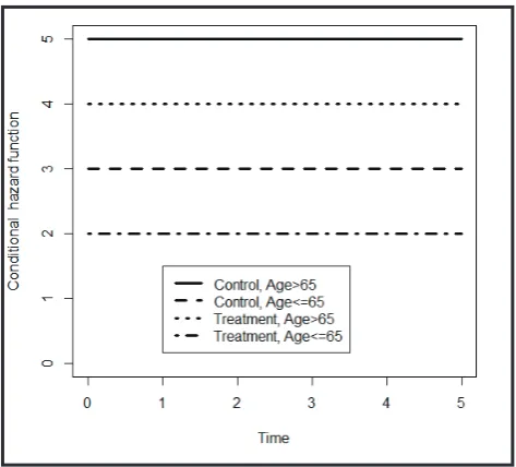
Simpson’s paradox may also occur in time-to-event data. [8] Suppose we have two treatment groups (denoted by X1: treatment (1)/ control (0)). We consider two age groups X2= 1 (or 0) if age is ≤ 65 (> 65) years. Suppose the hazard function of the life time T of patients given the treatment and age categories are
h(t│X1=0,X2=0)=5,h(t│X1=0,X2=1)=3, h(t│X1=1,X2=0)=4,h(t│X1=1,X2=1)=2.
Furthermore, we assume that the distribution of age categories of treatment groups are
Pr{X1=0,X2=0}=0.1, Pr{X1=0,X2=1}=0.9, Pr{X1=1,X2=0}=0.9, Pr{X1=1,X2=1}=0.1.
It is obvious that within each age category, the hazard function of the treatment groups is always below that of the control group. Figure 1 shows the hazard functions of two treatment groups within each age category. It is clear that treatment does a better job than control.
The marginal hazard functions of two treatment groups are
h(t│X1=0)=(0.5e-5t+2.7e-3t)/(0.1e-5t+0.9e-3t ), h(t│X1=1)=(3.6e-4t+0.2e-2t)/(0.9e-4t+0.1e-2t ). Figure 2 shows the marginal hazard function of two treatment groups after integrating out the age. In Figure 1, the hazard ratio of treatment versus control is a constant within each age category. However, the marginal hazard ratio is not a constant any more. This may cause some confusion especially if the follow-up time is censored at some time point . In that case, the estimated hazard function of the treatment group may be much higher than the control group, although this may not be what was expected.
5. Conclusion
Simpson’s paradox is very common in observational studies due to effects of confounding. In this paper, we
copyright.
on September 12, 2020 by guest. Protected by
Figure 1. Hazard functions in different age categories
Figure 2. Marginal hazard functions of two treatment groups
used some examples to show how this phenomenon can occur for continuous, categorical and survival outcomes. If the confounding effects are not addressed appropriately, conclusions obtained from statistical analyses may be totally wrong. The study of Simpson’s paradox, or more generally, of the effects of confounders, forms the rubric of the theory of causal inference, which is especially relevant in the error of big data as most data are observational in nature and confounders can obscure relationships of interest if not addressed.
Funding statement
This study received no external funding.
Conflict of interest statement
The authors have no conflict of interest to declare.
Authors’ contributions
Bokai Wang, Changyong Feng, and Xin M. Tu: theoretical derivation
Pan Wu and Brian Kwan: manuscript drafting
概述:辛普森悖论普遍存在于很多领域。它具有数据
的条件性和边缘性解释之间的不一致特征。在本文中, 我们通过一些例子来阐述辛普森悖论是如何在连续性、
分类和时间 - 事件数据中产生的。
关键词:条件期望;比值比;时间 - 事件分析
辛普森悖论的范例
Wang B, Wu P, Kwan B, Tu X, Feng C
References
1. Simpson EH. The Interpretation of Interaction in Contingency Tables. J R Stat Soc Series B. 1951; 13: 238-241
2. Yule GU. Notes on the Theory of Association of Attributes in Statistics. Biometrika. 1903; 2 (2): 121-134. doi: https://doi. org/10.1093/biomet/2.2.121
3. Heydtmann M.The nature of truth: Simpson’s Paradox and the limits of statistical data. QJM. 2002; 95(4): 247-249. doi:
https://doi.org/10.1093/qjmed/95.4.247
4. Lerman K. Computational social scientist beware: Simpson’s paradox in behavioral data. J Comput Soc Sc. 2018; 1: 49-58. doi: https://doi.org/10.1007/s42001-017-0007-4
copyright.
on September 12, 2020 by guest. Protected by
5. Malinas G, Bigelow J. Simpson’s Paradox.Edward N. Zalta (ed.) The Stanford Encyclopedia of Philosophy (Fall 2016 Edition). Available from: https://plato.stanford.edu/archives/ fall2016/entries/paradox-simpson
6. Rosenbaum P R. Observational Studies (2nd ed.). New York: Springer; 2002
7. Pearl J. Causality (2nd ed.). Cambridge University Press; 2009 8. Cox DR. Regression Models and Life-Tables. J R Stat Soc
Series B Stat Methodol. 1972; 34(2): 187-220
Bokai Wang obtained his BS in Statistics from the Nankai University in 2010 and his MS in Applied Statistics from the Bowling Green State University (Bowling Green, OH) in 2012. He is currently a PhD student in Statistics at the University of Rochester. His research interests include but are not limited to Survival Analysis, Causal Inference, and Variable Selection in Biomedical Research. As of now he has
published 7 papers in peer reviewed journals.
copyright.
on September 12, 2020 by guest. Protected by