IJMGE
Int. J. Min. & Geo-Eng.
Vol.48, No.2, December 2014, pp.191-199.
191
The Use of Robust Factor Analysis of Compositional Geochemical
Data for the Recognition of the Target Area in Khusf 1:100000 Sheet,
South Khorasan, Iran
Majid Keykha Hoseinpoor, Ahmad Aryafar
*Department of Mining, Faculty of Engineering, University of Birjand, Iran
Received 5 Nov 2014; Received in revised form 4 Dec 2014; Accepted 15 Dec 2014 *Corresponding author:[email protected]
Abstract
The closed nature of geochemical data has been proven in many studies. Compositional data have special properties that mean that standard statistical methods cannot be used to analyse them. These data imply a particular geometry called Aitchison geometry in the simplex space. For analysis, the dataset must first be opened by the various transformations provided. One of the most popular of the applied transformations is the log-ratio transform. The main purpose of this research is to identify the anomalous area in the Khusf 1:100000 sheet which is located in the western part of Birjand, South Khorasan province. To achieve the goal, a dataset of 652 stream sediments geochemically analysed for 20 elements was collected. In practice, the geochemical data were first opened by CLR transformation and then the range correlation coefficient (RCC) ratio was calculated and mapped. In consequence, the robust factor analysis for compositional data was used to separate the elements, mostly in the high-value regions obtained by the method of RCC. Finally, the priority of anomalies was specified using weighted catchment analysis. The above procedures led to the recognition of some anomaly zones for elements of Cu, Bi, Sb, Ni and Cr in the study area. Such results can be useful for designing an appropriate exploratory plan for semi-detailed and detailed exploration steps.
Keywords:compositional data, Iran, log-ratio transform, RCC, stream sediment.
1. Introduction
The processing of geochemical data for detecting multivariate geochemical patterns or signals associated with mineralization in support of mineral resource exploration is challenging [1]. Factor analysis, which was popularized by Charles Spearman in the early 1900s, has become one of the most widely
192 dimensionality of the data to these few representative factors, and therefore aims to summarize the multivariate information in a compact form [3]. In general terms, when using factor analysis as an exploratory method, the results will show properties inherent in the multivariate data, which should, however, be carefully checked with other methods, preferably those with less complicated visualization tools [4]. A stream sediment geochemical dataset is an example of a closed number system because it contains compositional variables that are parts of a whole [5]. In the last five decades, several researchers have discussed the problems in statistical analysis of closed number systems such as compositional datasets [6-18]. In practice, log-ratio transformations are commonly employed in geochemical data processing to open closed systems for better understanding of realistic relationships among compositions [5, 15, 19-21]. Log-ratio transformations process compositional data through two treatments: defining ratios of compositional parts and taking logarithms of the ratios. The former is used to decompose the closure effect by selecting proper divisors, while the latter is used to make the transformed compositional data log normally distributed [22]. When applying factor
analysis to compositional data, it is crucial to apply an appropriate transformation. A log-transformation will often reduce data skewness, but it does not accommodate the compositional nature of the data [23]. In general, three main log-ratio transformations are frequently applied to compositional data: (1) additive log-ratio (ALR) transformation [6, 7, 9, 22]; (2) centred log-ratio (CLR) transformation [6, 7, 9, 22]; and (3) isometric log-ratio (ILR) transformations [15, 22].
2. Study area and geochemical data
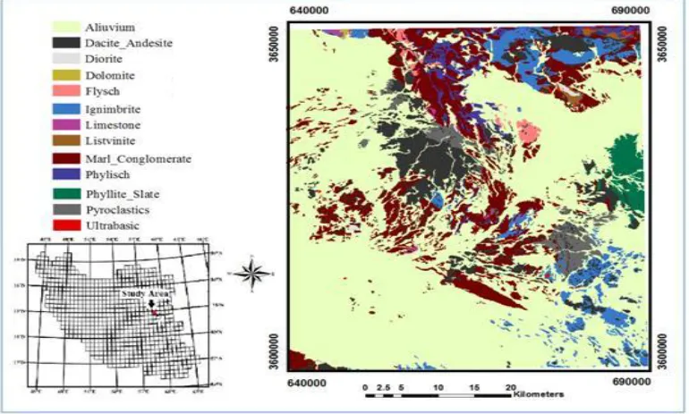
The study area, with a surface of 2500km2 covering Khusf district on 1:100,000 scale quadrangle maps, is located in the western part of South Khorasan Province, East Iran. Due to its location in the northern part of the Central Lut Block, this area has inherited characteristic arid conditions [24]. There are widespread exposures of Late Cretaceous-Early Tertiary sedimentary rocks and Cenozoic volcanism. Elevated areas and mountain ranges are arranged in the north and north-eastern part, while in the other parts, the topography is dominated by abundant irregular hills and intervening alluvial plains within which scattered, higher and isolated volcanic bodies may be seen (Fig. 1).
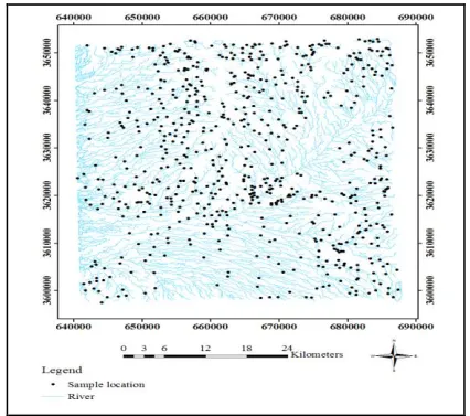
193 The oldest rocks in the area are upper Palaeozoic which are restricted to small fractured and faulted fragments of the central Iranian Palaeozoic platform and are exposed as an anti-form in the north-west of the map. The lithology units of the study area are Flysch-type sediments, marl and limestone. During mid-Eocene, non-volcanic deposits including agglomerate, ignimbrite, marl and tuff have been found in the north-west and south-west corner of the sheet. Eocene-Oligocene volcanic rocks including andesite, tuff and dacitic andesite have been spread in study area. Eocene-Oligocene dacite, silicified volcanic rocks and Oligo-Miocene rhyolites and dacites have been formed in sheet. To identify a promising area in the Khusf 1:100000 sheet, a drainage geochemical survey was carried out and 652 geochemical samples were taken. Fig. 2 shows the stream sediment samples’ location in the study area. The minus 80-mesh fraction of the stream sediments was analysed for 20 elements include Au, W, Mo, Zn, Pb, Ag, Cr, Ni, Bi, Sc, Cu, As, Sb, Cd, Co, Sn, Ba, V, Sr and Hg, and three oxides, MnO, TiO2 and Fe2O3.
Fig. 2. S tream sediment samples’ location in Khusf 1:100000 sheets
3. Methods
3.1. Log-ratio transformation
The closed nature of geochemical data has been proven in many studies [12, 22]. Compositional data have special properties that mean that standard statistical methods cannot be used to analyse them [5]. Euclidean
space is not suitable for compositional data or the limitations of a fixed sum. These data imply a particular geometry called Aitchison geometry in simplex space [23]. To analyse them, the dataset must first be opened by the various transformations provided.
Transforms such as this LR transform are of a family that was first presented by Aitchison (1986). Statistical methods applied to the transformed data and the results back-transform them to the original space [23].
The sample space of compositional data is the simplex that for D-part X
x ,...x1 D
composition is defined as [9]:
(1)
1 0 1 2 1
D D
D i i i
S X x ,...,x x ,i , ,...,D ;
x kThe positive constant κ with respect to measurement of the data unit differs from 1 in the case of proportions, 100 (percentages) or 106 (mg/kg).
To transform the data to the Euclidean space, the family of log-ratio transformations from the simplex SD to the Euclidean real space was proposed [25]:
Additive log-ratio (ALR) transformations, where for a D-part composition x the ALR transformation is defined as [9]:
(2)
i
1 2 1
i D
x
alr x y ln i , ,... , D x
Centred log-ratio (CLR) transformations, where for a D-part composition x the CLR is defined as [9]:
(3)
1
1
1 2 1
i D
i i
x
clr x y ln i , ,... , D
x
Isometric log-ratio (ILR) transformations, where for a D-part composition x an ILR transformation is defined as [15]:
(4)
1
1 2 1
1
i
i D i D
j j i
x D i
ilr x y ln i , ,...,D
D i x
194 3.2. Range correlation coefficient
Analysis of the dataset using the range correlation coefficient (RCC) method was first introduced and applied by Valls (2008). This method is based on the compositional nature of geochemical stream sediment data. The use of this method before performing other analysis in order to obtain an overview of the situation based on the correlation of a set of elements has been suggested [26]. The stages of the procedure are as follows:
Open the dataset by log-ratio transforms Calculate the correlation matrix of
elements
Calculate the critical value of the dataset to determine the significance of the obtained correlations using equation (5):
(5)
2
2
1
c
r
t
* n
r
where, tc is the critical value of dataset, r is
correlation and n is amount of data
Identify the significant amounts of critical value. It is common practice in geology to specify that for n > 30 and a probability of 0.05 (95 %), if tc> 3, then
the correlation is significant [26]
Calculate fraction of RCC based on the significant critical values
Plot the RCC map.
3.3. Robust factor analysis
Factor analysis (FA) is one of the most important multivariate statistical methods [27] that is widely used for pre-processing and data dimension reduction, and the resulting components are used for multivariate statistical analysis [28, 29]. Factor analysis is traditionally used to discover a number of factors (new variables) that cannot be observed directly [3]. For the random vector y to the D-dimensional real space, the factor analysis model is defined as:
(6)
y
f
e
with the factors f of dimension k<D, the error term e, and the loadings matrix . Multiple related variables can be converted into uncorrelated factors based on a covariance or correlation coefficient matrix [30, 33]. FA relies on the estimation of the correlation
matrix and this estimator is sensitive to outlier value. This classical approach is good if the data are multivariate normally distributed [2, 25, 34]. But we know in reality data distribution deviates from this ideal distribution and the results achieved without eliminating these values are associated with error [16]. To resolve this problem, the use of robust statistical methods has been proposed [35].
For a P-dimensional multivariate sample, xi(x1,…,xn), the outliers [36] are detected based
on Mahalanobis distance (MD):
(7)
1
1 2
1
i i i
MD X X T C X T i ,...,n
where T and C are estimations of location (i.e., the multivariate arithmetic mean or centroid) and scatter (i.e., covariance matrix), respectively [19, 35, 37]. The choice of the estimators is crucial for the quality of multivariate outlier detection [19] and on the other hand, we know that classical estimators of the arithmetic mean and sample covariance matrix are sensitive to the distribution of outliers [19, 48]. For this reason, robust counterparts need to be taken. A popular choice is the MCD (minimum covariance determinant) estimator [38]. For the multivariate normally distributed data, the Mahalanobis distance is approximately chi-square distributed with P degrees of freedom ( 2
p
x ) [22, 39]. This distribution might also be considered for the robust case, and a quantile, e.g., 0.975, can be used as a cut-off value separating regular observations from outliers [34].
The log-ratio transformations dealing with the closure effect of compositional exploratory data [9, 19, 40, 47] can be used to investigate the geochemical data as well. In order to give an appropriate interpretation of the loadings and scores, the obtained results of the compositional factor analysis should be back-transformed in CLR space [34].
3.4. Weighted catchment analysis
195 influence of each sample [42, 43]. This method provides a better representation of the data and is very useful in identifying local anomalies [44]. This approach is based on the association of an area of statistical representativeness with each sample, and on the assumption that the concentrations measured in the stream sediments can be considered as average reference values for this area [43]. To estimate the amount of local background in each catchment, the analysis of the weighted mean univariate-element concentrations due to lithology was presented by Carranza (2008). This method has been described by Equation (8).
(8)
1 1
n n
j i i ij i ij
M
Y X
Xwhere Mj is concentration in each of the j
(=1,2,…,m) lithological units of i (=1,2,…,n) sample catchment basins. Yj represents
univariate-element concentrations in the stream sediment sample and Xij is the area of
each of the j lithological units [41]. Then, the local background concentration of element ( ) due to lithology can be estimated as (9):
(9)
1 1
m m
j i j ij j ij
Y
M X
XPositive or negative geochemical residuals ( ) can be interpreted as enrichment or depletion, respectively, of the element concentration in stream sediments. But only positive values are processed further for dilution effect correction because they are of interest in mineral exploration [45].
4. Summary and discussion
To identify exploratory geochemical targets in Khusf 1:100000 sheet, the stream sediment data were first opened by CLR transformation and then the RCC ratio was calculated. The resulted fraction is:
(10)
22 20 2 3 19 17 16 15 9 2
Rcc
16 14 2 8
Bi Ni Cu Hg Fe O Zn As Sr MnO Sb Cr Co V Sc Cd W Ag Mo Pb Ba TiO Sn
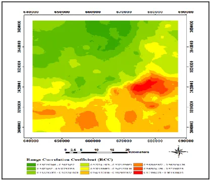
Later the RCC fraction (Eq. 10) was calculated for each observation to obtain a vector of RCCs in any coordinate of the samples. Finally, the vector was plotted as a map presented in Figure 3.
Fig. 3. The RCC map of Khusf 1:100000 stream sediment
The regions on the map that show high value of RCC are the elements gathered in the numerator and the regions with low values appear in the denominator. To determine the
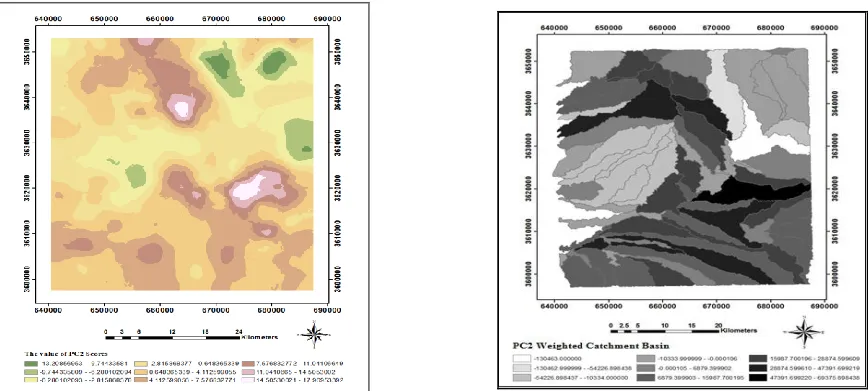
elements that are mostly in the high-value regions obtained by the method of RCC, the data were analysed using the robust factor analysis method for compositional data. After applying a robust factor analysis on the ILR-transformed data with four varimax rotated factors and back-transforming the results in CLR space using rgr package [46], the factor scores together with the weighted catchment basins (WCB) were mapped. As shown in the factor loadings (Fig. 4), the elements associated in the first factor with about 41 % of explained variation, including Ni, Zn, Bi, Cu, Hg and Fe2O3, are chalcophile elements related to the lithological units dacite, dacitic-tuff, dacitic volcanic dome and ignimbrite.
196 insight into the multi-elemental correlations in the study area. The factor analysis carried out in this study confirms that RCC can be a way to explore the most important paragenesis of
the region before performing any further complicated analysis. In order to evaluate the accuracy of the obtained results, anomaly checking was carried out by field trip.
Fig. 4. PC loading values for compositional data analysis
Fig. 5a. Distribution map of factor score F1: interpolated values (left) and WCB map (right)
197 Conclusions
The previous studies show that the geochemical data generally do not have a normal distribution, resulting in problems for the application of classical techniques, because these are based on the assumption of normal distribution. However, the discussed methods are based on the Euclidean space. They could not be used directly for processing geochemical data because the geochemical data are typical compositional data. Therefore, geochemical data should be opened prior to analysis; otherwise, biased results could be obtained. In the present research, the abovementioned approach was applied to a stream sediment geochemical dataset which was collected from the Khusf 1:100000 sheet, Birjand, South Khorasan, Iran. To achieve the goal, in the first step, the stream sediment data were opened using CLR transformation, and then the RCC ratio was calculated. In the second step, the data were analysed using the robust factor analysis method for compositional data. In the results of this application, the main extracted factor, which included Ni, Zn, Bi, Cu, Hg and Fe2O3 elements, explains more than 41 % of variation in the study area. As a main result, the factor analysis carried out in this study confirms that RCC can be a way to explore the most important paragenesis of the region before doing any further complicated analysis. In order to evaluate the accuracy of the obtained results, anomaly checking was carried out by field trip.
Acknowledgement
The authors would like to express their appreciation to the authorities of the South Khorasan Industry, Mine & Trade Organization, who provided the facilities for doing of this research. The financial support of the University of Birjand is gratefully acknowledged.
References
[1] Zuo, R. (2014). Identification of geochemical anomalies associated with mineralization in the Fanshan district, Fujian, China. Journal of Geochemical Exploration, 139, pp. 170-176. [2] Treiblmaier, H., Filzmoser, P. (2010).
Exploratory factor analysis revisited: How robust
methods support the detection of hidden multivariate data structures in IS research. Information & management, 47(4), pp. 197-207. [3] Filzmoser, P., Hron, K., Reimann, C. (2009a). Principal component analysis for compositional data with outliers. Environmetrics, 20(6), pp. 621-632.
[4] Reimann, C., Filzmoser, P., Garrett, R., &Dutter, R. (2008). Statistical data analysis explained: applied environmental statistics with R: John Wiley & Sons.
[5] Carranza, E.J.M. (2011). Analysis and mapping of geochemical anomalies using logratio-transformed stream sediment data with censored values. Journal of Geochemical Exploration, 110(2), 167-185. Geochemical Exploration, 140, pp. 96-103.
[6] Aitchison, J. (1981). A new approach to null correlations of proportions. Journal of the International Association for Mathematical Geology, 13(2), pp. 175-189.
[7] Aitchison, J. (1983). Principal component analysis of compositional data. Biometrika, 70(1), pp. 57-65.
[8] Aitchison, J. (1984). The statistical analysis of geochemical compositions. Journal of the International Association for Mathematical Geology, 16(6), pp. 531-564.
[9] Aitchison, J. (1986). The statistical analysis of compositional data (Vol. 25): Chapman & Hall. [10] Aitchison, J. (1999). Logratios and natural
laws in compositional data analysis. Mathematical Geology, 31(5), pp. 563-580. [11] Aitchison, J., Barceló-Vidal, C.,
Martín-Fernández, J., Pawlowsky-Glahn, V. (2000). Logratio analysis and compositional distance. Mathematical Geology, 32(3), pp. 271-275. [12] Buccianti, A., Pawlowsky-Glahn, V. (2005).
New perspectives on water chemistry and compositional data analysis. Mathematical Geology, 37(7), pp. 703-727.
13] Chayes, F. (1960). On correlation between variables of constant sum. Journal of Geophysical research, 65(12), pp. 4185-4193. [14] Egozcue, J. J., Pawlowsky-Glahn, V. (2005).
Groups of parts and their balances in compositional data analysis. Mathematical Geology, 37(7), pp. 795-828.
198
compositional data analysis. Mathematical Geology, 35(3), pp. 279-300.
[16] Filzmoser, P., Hron, K., Reimann, C. (2009 b). Univariate statistical analysis of environmental (compositional) data: problems and possibilities. Science of the Total Environment, 407(23), pp. 6100-6108.
[17] Miesch, A. (1969). The constant sum problem in geochemistry, Springer, pp. 161-176.
[18] Thió-Henestrosa, S., Martín-Fernández, J. (2005). Dealing with compositional data: the freeware CoDaPack. Mathematical Geology, 37(7), pp. 773-793.
[19] Filzmoser, P., Hron, K., Reimann, C. (2012). Interpretation of multivariate outliers for compositional data. Computers & Geosciences, 39, pp. 77-85.
[20] Gallo, M., Buccianti, A. (2013). Weighted principal component analysis for compositional data: application example for the water chemistry of the Arno River (Tuscany, central Italy). Environmetrics, 24(4), pp. 269-277. [21] Verma, S. P., Guevara, M., Agrawal, S.
(2006). Discriminating four tectonic settings: Five new geochemical diagrams for basic and ultrabasic volcanic rocks based on log—ratio transformation of major-element data. Journal of Earth System Science, 115(5), pp. 485-528. [22] Wang, W., Zhao, J., Cheng, Q. (2013). Fault
trace-oriented singularity mapping technique to characterize anisotropic geochemical signatures in Gejiu mineral district, China. Journal of Geochemical Exploration, 134, pp. 27-37. [23] Filzmoser, P., Hron, K. (2009). Correlation
analysis for compositional data. Mathematical Geosciences, 41(8), pp. 905-919.
[24] Arjmandzadeh, R., Karimpour, M., Mazaheri, S., Santos, J., Medina, J., Homam, S. (2011). Sr–Nd isotope geochemistry and petrogenesis of the Chah-Shaljamigranitoids (Lut Block, Eastern Iran). Journal of Asian Earth Sciences, 41(3), pp. 283-296.
[25] Filzmoser, P., Hron, K., Reimann, C. (2010). The bivariate statistical analysis of environmental (compositional) data. Science of the Total Environment, 408(19), pp. 4230-4238. [26] Ricardo, A. V. (2008). Why, and how, we should use compositional data analysis , A Step-by-Step Guide for the Field Geologists (S. Parker Ed.). Toronto, Ontario.
[27] Reimann, C., Filzmoser, P., Garrett, R. G.
(2002). Factor analysis applied to regional geochemical data: problems and possibilities. Applied Geochemistry, 17(3), pp. 185-206. [28] Johnson, R., Wichern, D. (2007). Applied
Multivariate Statistical Analysis. Prentice-Hall, 6nd Edition.
[29] Filzmoser, P., Hron, K., Reimann, C., Garrett, R. (2009 c). Robust factor analysis for compositional data. Computers & Geosciences, 35(9), 1854-1861.
[30] Cheng, Q., Bonham-Carter, G., Wang, W., Zhang, S., Li, W., Qinglin, X. (2011). A spatially weighted principal component analysis for multi-element geochemical data for mapping locations of felsic intrusions in the Gejiu mineral district of Yunnan, China. Computers & Geosciences, 37(5), pp. 662-669. [31] Horel, J. (1984). Complex principal component analysis: Theory and examples. Journal of climate and Applied Meteorolo gy, 23(12), pp. 1660-1673.
[32] Jolliffe, I. (1991). Principal component analysis: Wiley Online Library.
[33] Loughlin, W. (1991). Principal component analysis for alteration mapping. Photogrammetric Engineering and Remote Sensing, 57(9), pp. 1163-1169.
[34] Filzmoser, P., Hron, K., Reimann, C. (2005). Principal component analysis for compositional data with outliers. Environmetrics, 20(6), pp. 621-632.
[35] Filzmoser, P., Hron, K. (2008). Outlier detection for compositional data using robust methods. Mathematical Geosciences, 40(3), pp. 233-248.
[36] Barnett, V., Lewis, T. (1984). Outliers in statistical data. Wiley Series in Probability and Mathematical Statistics. Applied Probability and Statistics, Chichester: Wiley, 1984, 2nd ed., 1. [37] Barceló, C., Pawlowsky, V., Grunsky, E. (1996).
Some aspects of transformations of compositional data and the identification of outliers. Mathematical Geology, 28(4), pp. 501-518. [38] Rousseeuw, P.J., Driessen, K.V. (1999). A
fast algorithm for the minimum covariance determinant estimator. Technometrics, 41(3), pp. 212-223.
[39] Maronna, R., Martin, R., Yohai, V. (2006). Robust Statistics: Theory and Methods: Wiley, New York.
199
Simplicial geometry for compositional data. Geological Society, London, Special Publications, 264(1), pp. 145-159.
[41] Carranza, E. J. M. (2008). Geochemical anomaly and mineral prospectivity mapping in GIS (Vol. 11): Elsevier.
[42] Bonham-Carter, G., Rogers, P., Ellwood, D. (1987). Catchment basin analysis applied to surficial geochemical data, Cobequid Highlands, Nova Scotia. Journal of Geochemical Exploration, 29(1), pp. 259-278. [43] Spadoni, M. (2006). Geochemical mapping
using a geomorphologic approach based on catchments. Journal of Geochemical Exploration, 90(3), pp. 183-196.
[44] Yousefi, M., Carranza, E. J. M., Kamkar-Rouhani, A. (2013). Weighted drainage catchment basin mapping of geochemical anomalies using stream sediment data for mineral potential modeling. Journal of Geochemical Exploration, 128, pp. 88-96.
[45] Abdolmaleki, M., Mokhtari, A. R., Akbar, S., Alipour-Asll, M., Carranza, E. J. M. (2014). Catchment basin analysis of stream sediment geochemical data: Incorporation of slope effect. Journal of Geochemical Exploration, 140, pp. 96-103.
[46] Garrett, R.G. (2013). The ‘rgr’package for the R Open Source statistical computing and graphics environment-a tool to support geochemical data interpretation. Geochemistry: Exploration, Environment, Analysis, 13(4), pp. 355-378.
[47] Pawlowsky-Glahn, V., Egozcue, J. (2006). Compositional data and their analysis: an introduction. Geological Society, London, Special Publications, 264(1), pp. 1-10.