A Novel Approach for Job Scheduling and Load Balancing in Grid Computing Environment

(1)

A

N

O

V

E

L

A

P

R

O

A

C

H

F

O

R

J

O

B

S

C

H

E

D

U

L

I

N

G

A

N

D

L

O

A

D

B

A

L

A

N

C

I

N

G

I

N

G

R

I

D

C

O

M

P

U

T

I

N

G

E

N

V

I

R

O

N

M

E

N

T

K

.

J

a

i

r

a

m

N

a

i

k

11

,

D

r

.

A

.

J

a

g

a

n

22

,

D

r

.

N

.

S

a

t

y

a

N

a

r

a

y

a

n

a

33

1

Assistant Professor, Dept of CSE, Vasavi College of Engineering, Hyderabad, Telangana 2

Professor, Dept of CSE, Dr. BV Raju Institute of Technology, Narsapur, Telangana 3

Professor, Dept of CSE, Nagole Institute of Tech & Science, Hyderabad, Telangana

Corresponding author: K. Jairam Naik, [email protected]

ABSTRACT: Since the grid is emerging all over the

internet, there comes a need for optimal job scheduling and load balancing approaches that takes various characteristics of the grid environment into consideration. Our principal seek is to present a novel fault tolerant approach for job scheduling and load balancing. Our approach called as NovelAlg_FLB mainly focuses on the architecture of the grid, bandwidth of the network, delay caused by communication, availability of resources, heterogeneity of computer resources and other features of jobs. This approach culminates the strength of various other algorithms such as load based and cluster based algorithms. The primary aim of this research is to schedule jobs in such a way that the job’s task delivers their response in minimum time. Also, this approach ensures that the computing nodes are optimally used. The secondary aim of this approach is to reduce complexity and the reduction in the total number of additional communication lines due to load balancing. We have used a java based simulation toolkit called grid GridSim to conduct the simulation of the proposed approach. Experimental results prove that our approach works extremely well in a huge and complex grid environment.

KEYWORDS: Computing Grid, Job Scheduling, Load

Balancing, Fault Handler, Completion time, Resubmission time.

1.INTRODUCTION

Grid computing is the current trending distributed computing technology as it makes use of heterogeneous resources that are physically as well as geographically dispersed all over the world. Grid computing makes use of heterogeneous resources that native to geographically distributed administrative firm to achieve one common objective. A heterogeneous network, Wide Area Network (WAN) interconnects the various resources. There is a need for a heterogeneous network because the bandwidth in a grid environment varies from one link to another. Delay and bandwidth limited communication that gradually result in delays in inter-node communications and load exchange pose a severe problem to any distributed computing environment (DCE). A grid environment is more complex than a DCE. Some factors that make it complex are: the

behaviour of the processors is unpredictable; their speeds may change over time and computers may connect and disconnect upon their wishes. Thus, a proper mechanism is needed to get the best welfare from the grid.

There are two types of grid systems namely compute grids and data grids. The primary goal of compute grids is to provide compute cycles (i.e., processors) while that of data grids is to handle data that is distributed over various geographic locations through the grid. The type of grid affects its architecture and the various services provided by the resource management. Job scheduling and load balancing are two factors, which if improperly implemented poses a threat to the grid environment. A real job scheduling algorithm ensures that the grid meet the deadlines given by the client while making the best used of all the available resources.

1.1.Literature survey

Job scheduling algorithms are required to maintain load balance in the system and thus improve the overall performance of the system. In the grid environment, the resources vary with time as they are provided by remote and idle computers whose conditions are not stable. Moreover, new resources join and old resources leave the grid environment unpredictably thus leaving the grid unstable. Thus any job scheduling algorithm should be designed bearing in mind all the complex factors and conditions that affect the grid and the algorithm should also vary dynamically along with the grid. Consequently comes the need of an efficient algorithm that suits the dynamic variant environment of the grid.

(2)

resource and the heavily loaded resource is as least as possible thus ensuring that the load is equally assigned. Load balancing algorithms are of three types: centralized, decentralised algorithms and hierarchical algorithms.

In centralized approach, one resource determines how all the jobs can be scheduled to the present available resources. In decentralized approach, each resource is allowed to make all the load balancing decisions. In a hierarchical approach, as the name suggests , the schedulers are divided and organized into a hierarchy. Lower level resources are scheduled at lower level and the higher level ones are scheduled at higher level as per their hierarchical position. This approach can be seen as a combination of both centralized and decentralized approaches.

1.2.Related work

Based on the type of information on which load balancing decisions are made, scheduling algorithms are once again classified as static, dynamic or hybrid algorithms. Static algorithms make use of all the earlier available information i.e., available resources, communication network and the characteristics of jobs. Static algorithms also assume that all the information stated above remains the same thus cannot be in par with the dynamic nature of the grid environment. However dynamic algorithms take into consideration the dynamic aspects of the grid in contrast to its counterpart, static algorithms. Adaptive algorithms [WR93] are a special case of dynamic load balancing algorithms. In order to adapt to the changing environment, dynamic algorithms make use of four policies namely information, location, transfer and selection whenever any kind of load imbalance is created.

Information policy, as the name suggests maintains an up-to-date information of each resource. Load information of a resource mainly determines whether a resource is qualifies as a sender or as a receiver. Location policy is for selecting resource partners for a job transfer transaction. Transfer policy is related to the dynamic aspects and the selection policy is used to select jobs that are queued. The main aim of selection policy is to select a job that causes least overhead upon transfer, and has more affinity to the resource it is being tranferred to.

Resource failures do occur in a grid and have an adverse effect on the application. Thus comes the need for algorithms that also maintain fault tolerance. Job replicas are used to schedule such applisations. There are two approaches to replication: active replication and passive replication.

1. Active Replication: Multiple replicas of each job are scheduled and they are run on different processors in parallel. This approach however leads to space redundancy.

2. Passive Replication: For each job, a back-up is scheduled in another processor. The backup is executed whenever a fault occurs in the primary [Nae99]. This approach is guaranteed to recover from any failure that may affect the system. An advantage of this approach is that only TWO copies are scheduled. There were TWO techniques used in order to schedule primary and backup jobs.

(i). Backup jobs are scheduled by backup overloading. This is generally used when multiple primary jobs are scheduled for the same slot and guarantees the efficient use of processor.

(ii). The second technique is the deallocation of resources that are no longer required. Algorithms using above techniques have certain common features ([Nae99], [QJ06]):

1. Independent jobs with deadlines. 2. Homogeneous system architecture. 3. Each can handle one failure of process

In [JVS12], K Jairam Naik et al. balanced the load in the grid by grouping the resources in to levels as per their success rate and speed. Where, the main consideration was the success rate history of each resource to determine a suitable resource for the job, and to take scheduling decision thereafter. Based on the resource speed requirement, the job is scheduled to the resource of a specific level. Once the job is scheduled on the selected resource, it is removed from the available resource set. When the resource finishes the assigned job then it moves to the set of available resources. If this resource completes the allotted job in estimated time, then its success rate value is incremented by 1, otherwise -1, this value is considered for determining successful resource in the future. With this approach no resource is overloaded. In [JS13], K Jairam Naik et al. considered fault rate of resources and job QOS requirements to determine resource Performance Indicator (PI). PI value decides a suitable resource for job, and to take scheduling decision thereafter. Where, lower the PI gives the resource with less failure tendency.

(3)

and is completely unrealistic in large scale grid environment. A well-designed information exchange scheduling scheme is adopted to enhance the efficiency of the load balancing model.

1.3.Our contributions

This section mainly gives the details of the specifications and also the achievements of the algorithm proposed by us.

1. The various factors of the grid, i.e architecture, unpredictability, network bandwidth, heterogenity of resources are all dealt with in this algorithm to generate a fault tolerant load balancing algorithm.

2. Overhead caused due to collection of information of each resource is reduced by this algorithm.

3. Messages are exchanged between resources in a well designed fashion thus improving the overall performance of the system. An algorithm similar to piggybacking [Son94] and [LZ07], that supports mutual request response policy is used to exchange messages.

We have proposed an extended version of the fault tolerant hybrid load balancing strategy namely AlgHybrid_LB policy specified in Jasma Balasangameshwara [JN12].

The following sections deal with the design of the proposed algorithm. The following section provides an overview of the system model. The proposed algorithm is explained in detail in Section 3 while section 4 provides the experimental results which proves that the proposed algorithm is better than the existing algorithms. Conclusion and work which can be done as an extension to this in future are explained in section 5.

2. SYSTEM MODEL

2.1.Design of system environment

We have used a simple but realistic approach to describe the grid environment. We assume that the grid consists of a set of clusters P; where P=P1,P2,………Pn which are connected to a network through links which also have different speeds. In a grid, a site can contain any number of machines or computing nodes and similarly a machine can include any number of processing elements abbreviated as PE’s. However in our simulation, we assume that each site can contain only one machine and each machine may include single or multiple processing entities. This hypothesis guarantess that there is no loss of generality and emphasizes all the ideas of the proposed algorithm. All processors need not have the same processing power irrespective of whether they

belong to the same network or different networks. The Grid scheduler, which can also be called as the heart of the grid environment is a software component that is present on each site. The grid scheduler plays an important role in the grid as it manages all the client requests and sends the appropriate resources to handle the requests. The grid scheduler also accepts ―join‖ requests from the idle sites and assigns them tasks appropriately.

The environmental conditions that need to be satisfied to build a grid environment are given below:

(1) Whenever a new site joins the grid, the site has to provide the grid with its hardware information i.e., speed of CPU, size of memory, internal registers etc.

(2) Every grid has a grid scheduler whose main task is to administer the state of all the sites present in the grid.

(3) The grid scheduler should provide the user with the required hardware information of each resource they asked for it [T+05].

(4) The user can provide accurate details of the information related to resources that are in high demand.

(5) The current level of resource contribution and the current time taken by a resource to process the job are recorded and taken as reference for scheduling in the future.

Sites play an important role in the execution of job through message passing. When a site is idle and can provide its resources to the grid, it sends a ―join‖ message to the grid scheduler and provides all of its hardware information to the grid scheduler. In a similar manner, every site sends an ―exit‖ message to the grid scheduler of its nearest neighbour when it can no longer provide any resource.

2.1.1. The grid scheduler

As mentioned above, the main role of the grid scheduler is to manage jobs. Jobs which are idle and can be used are placed in the ready queue and these jobs are assigned when required for processing. All the tasks that are performed by the grid scheduler are given below:

(i) Ensures that all the sites provide resources for the grid environment.

(ii) Gathers relevant information such as CPU utilization, remaining memory, etc. from all the sites taking part in the grid.

(iii) When a client sends a job request to the scheduler, it sends to the load balancing decisionmaker a set of adjoining sites that satisfy all the job requirements and resource characteristics.

(4)

or in a remote site and accordingly transfer the job to the dispatcher. The job dispatcher then sends the job to a fault detector which monitors the state of sites. Whenever a site fails, the fault detector sends a failure message to the fault manager which reschedules the job upon receiving the failure message.

2.1.2. Determining the effective sites

Since the sites are dynamic and can switch between an idle state and busy state unpredictable resource availability shouldn’t be the only factor that is considered. Other factors such as rate of job completion, site’s historic level of contribution, etc. should also be considered to select the most effective set.

(1)

(2) where,

xij = value of the variable i in site j; f(xij) = function value of variable i in the site j; Vj = estimated value of site j; i = variable i adopted in this function value; j = the computing node j in the grid ; N = total number of sites; wi = each variable’s weight value. To overcome the above drawbacks, we propose a new parameter called value function (VF) to estimate the value of each site which is later used as a reference to estimate the set of effective sites.

2.1.3. Selection of site

A derived threshold is used by the grid scheduler to select an effective site. The sites that are present within this threshold are declared as effective and will be organised into a table that stores a list of all effective sites. It is important that the table be updated regularly as the changes in sites are unpredictable. If the table is not adjusted accordingly then the current state of sites is not known and can lead to disaster. Thus TWO appproached are employed to handle these kinds of situations:

(1) Stable grid environment

The table of effective sites is automatically updated when a site enters or leaves the system. (2) Unstable grid environment

When the state of sites in the grid environment continually alters, setting the threshold for the table frequently adds extra load on the grid scheduler. Hence when a site joins, table that holds information of effective sites is not updated right away, but when the site variation reaches the threshold is updated. The site is noted as unavailable in the site table after exit of an effective site.

2.1.4. Selecting resource of a site

Every site in the grid environment maintains the history of each resource local to it, in a service table called Resource information service (RIS). This service table provides resource characteristics such as speed, memory space, bandwidth, success or failure rate etc. This data is needed to be trust on a resource services. In our approach, to find the most suitable resource [JVS12] for the incoming requests we mainly focus on Success rate (SR) of a resource. A resource i is said to be success(s) if it complete the execution of allotted job in expected time, otherwise it is called as fail(f). For every successful execution of a job by the resource, its SR value is incremented by 1; otherwise SR value is decremented by 1. All the resources of a site irrespective of the machine, to which they belongs, are arranged in descending order of their SR values. A specific resource is picked up based on users QOS requirements.

The success rate of a resource for the assigned job is calculated as

where,

Nsi, = Number of time the resourcei successed. Nfi = Number of time the resourcei failed to execute the submitted job in deadline.

For every job assigned to resourcei of a site, the Nsi, Nfi values are calculated by Success rate Calculator SRC and updated in RIS. The Nsi value of resourcei is incremented by 1, if the resource finishes the execution in deadline; otherwise Nsi value is decremented by 1. The failure rate value ( ) of resourcei is determined as Since the job execution time is hard to predict, depending on the type of application, method [JVS12] are used to estimate the job execution time.

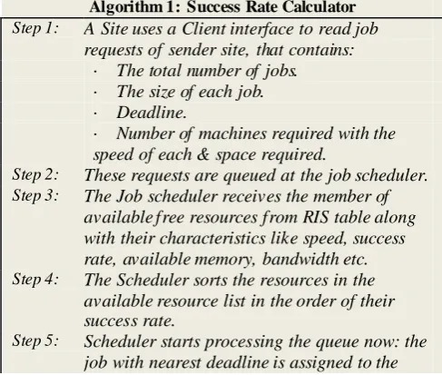
Algorithm 1: Success Rate Calculator

Step 1: A Site uses a Client interface to read job requests of sender site, that contains:

· The total number of jobs.

· The size of each job.

· Deadline.

· Number of machines required with the

speed of each & space required.

Step 2: These requests are queued at the job scheduler.

Step 3: The Job scheduler receives the member of

available free resources from RIS table along with their characteristics like speed, success

rate, available memory, bandwidth etc. Step 4: The Scheduler sorts the resources in the

available resource list in the order of their success rate.

Step 5: Scheduler starts processing the queue now: the

(5)

resource with highest SR value. Step 6: If the resource completes job execution in

expected deadline

Step 7: SR:=SR+1 //SRC increments the success rate

of the resource by 1

else

SR:=SR-1 //SRC decrements the success rate

of the resource by 1

Step 8: Update the latest SR value of each resource in the RIS, to be referred in the next iteration Step 9: Until all jobs are completed Repeat Step 1 to

Step 8.

The success or failed execution of the job j on the resource i and other related information is gathered by the mobile agents and submitted to the Success rate Calculator (SRC). If the job j assigned to resource i finishes its execution in deadline, then the resource success rate is incremented by1 as SRi: =SRi+1; otherwise its success rate decremented by 1 as SRi: = SRi-1 as shown in Algorithm 1.

2.2.System model

The jobs arrive in a random order which follows a Poisson method with a random computational length following an exponential distribution in our work. We assume that they are computationally intensive. We also assume that all these jobs are mutually independent and they can be executed on any site with condition that the corresponding site can provide the jobs’ demand for resources of computation and amount of data transmission. At a point of time, each processor can execute only one job. Execution of job cannot be altered (i.e. cannot be interrupted/moved to another processor) during execution (Tables 1 and 2).

Table 1: Grid resource characteristics

Number of machines/site 3

Number of PEs/ machine 3

PE ratings 10 or 50 MIPS

Bandwidth 1000 or 5000 B/S

Table 2: Scheduling parameters and their values

Number of sites 500

Number of jobs 100–2500

Number of job replicas 3

Job length 100–50,000 MI

Input ﬁle size 100 + (10–40%) MB

utput ﬁle size 250 + (10–40%) MB

2.3. Policy for load balancing

The novel load balancing algorithm proposed by us combines the strong points of static load balancing policy and that of dynamic dynamic load balancing policy. Static load balancing policy assigns an effective site when a client process needs to be executed. However, dynamic load balancing policy

continuously adjusts the tables and the system until an equilibrium i.e., state of complete balance is reached. 2.2.1. Load balancing – Static

The minimum requirement of job’s needs should be considered while determining the threshold. All the sites that pass the threshold are considered to be effective. The value of a site is determined by considering two main factors, namely the site and the job. Those sites that have the highest value for VF provide the most stable resources.

2.2.2. Load balancing - Dynamic

The effectiveness of the grid varies from time to time due to the changes in the sites under study. As the site status varies, the assignment of various jobs in the grid should also vary accordingly. Such variations are identified and resolved in the following ways:

1. When the grid scheduler receives a message that a particular site can no longer provide its resources or if the site is overloaded the grid scheduler selects the next free site and assigns it. 2. If the execution of a job on one particular site

exceeds the expected execution time, the grid scheduler determines if the site is still effective. If the result is effective then the execution time is re-estimated and if ineffective, then the next site with highes value of effectiveness is assigned.

2.4. Fault system model

Any failure present in a site affects all its jobs temporarily or permanently. The backup is scheduled after the primary for each and every job and is executed when a failure occurs in the primary. It is guaranteed that only one job can encounter a failure, i.e, the backup is always guaranteed to succeed. This condition is has a 100% grantee due to the evidence that the minimum value of greedy time of failure (MTTF) is always greater than or equal to the execution time. Processor and job failures are detected using certain mechanisms such as fail signal and acceptance test [[GMM97], [HK03]].

If a primary executes successfully or completes executin within the estimated time then the backup is deleted. This action is called ―resource reclaiming‖ and is crucial so that the backup can be used for other new jobs.

3. DESIGNING A NOVEL LOAD BALANCING POLICY

(6)

However if static load balancing policy fails ie., the site is unable to complete the jobs assigned it within the deadlines, then dynamic load balancing policy is employed.

3.1. Static load balancing policy

The factors such as CPU capacity, memory size, load, transmission rate, past completion rate etc. are taken into consideration to calculate the price of VF. Despite many factors being considered, transmission rate is the most important one as it taken as one of the most important parameters to select a site. Moreover, transmission rate is also considered as threshold for selection of VF due to the afore mentioned reason. Historical statistics are used to determine the current time when the site can provide resources due to the unpredictable nature of the grid. The sites that are underloaded are now taken as the threshold for VF [LZ07]. All the above parameters used to determine VF are quantified using mathematical expressions as shown below:

(3)

CV is the remaining percentage of CPU capacity; CS is the site’s CPU computing capacity (MHz); CU is the usage of the site’s CPU.

MV = (MS-MU)/MS (4)

MV is the remaining memory percentage of the site; MS is space of the memory (MB) available and MU the memory usage:

RV = NR/DW (5)

RV is a site’s quantified rate of transmission; NR is the transmission rate of the site and DW is the bandwidth between the site and the grid scheduler. Equations 3 and 4 show the quantification of unused capacity of CPU and memory respectively. Network transmission rate is taken as the denomination to quantify transmission rate and is shown below in equation 5.

For each and every effective site Pi, there exists q number of effective neighboring sites LNSeti. This set is used by the grid scheduler to pic k the most effective neighboring site for off-loading jobs. For any site Pi, another site Pk is considered as the neighboring site of Pi if the quantified rate of transmision between Pi and Pk is α times within the quantified rate of transmission between Pi and the nearest effective. Another factor for considering a site Pk as the neighbor of Pi is that the load of Pi should always be less than that of Pk. All the other sites are sorted using the values of quantified transmission rate

and the site that is ranked first is considered the most effective site [LZ07].

(6)

where,

RVik = quantified rate of transmission from site Pi to Pk;

RVinearest=quantified rate of transmission from nearest site of site Pi to itself.

The distance coefficient α = 1.36 is found to produce extremely good results (the variations of this random value for experiments are provided later in the section).

3.1.1. Algorithm: First-come-first-serve

Suppose a grid system having m sites where each site is denoted by Pi and its capability is denoted denoted by Ci. Here, we use ₽ and ₵ to denote such a system and its corresponding capacity subsequently [L+09].

(7)

(8)

Each job j in the set of jobs J has an arrival time t, a virtual computation duration jd, two scheduled attributes: a opening time and an finish time stand for js and je, respectively. Hence, job Jj can be indicated as a tupple consisting of 4 elements and defined (jj, jdj, jsj, jej). The grid sceduler allocates a job to a certain site upon arrival.

(9)

(jjd, js, je) = {(jj, jdj, jsj, jej) | j=1, 2, …, n} (10) The execution time texej for each job Jj can be expressed and calculated as follows:

(11)

Since, every job has equal probability of being allocated to a particular site, the FCFS should compute and identify a site that can do the job in the smallest period of time and in the most efficient way.

(12)

It is proved that the time of completion of job is always equal to the sum of the earliest possible start time and execution time irrespective of the method used to select the jobs.

(7)

The earliest possible start time varies based on the number of jobs waiting the queue before the current job. If there is no job that is running on the chosen site ahead of job Jj’s arrival, then Jj can be executed immediately on this site.

(14)

3.2. Dynamic load balancing policy

If static load balancing policy fails to assign an effective site, then the dynamic load balancing policy is executed. The dynamic load balancing policy is implemented in terms of four other policies namely information policy, load adjustment policy, transfer, and selection policy.

3.2.1. Information policy

A site i uses a state object Oi to store the state information of all its neighboring sites. The main advantage of this state object is that it gives the load of the system at any instant without transferring any message. There is property list containing two properties namely load and time in each object item Oi[j]. At any instant, Oi[k].load denotes the load of site Pk. Similarly, Oi[k].time denotes the last modified time of the site Pk. The two values Oi[k].load and Oi[k].time need to be maintained properly and are updated through message passing algorithms [LZ07]. State information is exchanged through a mutual information feedback which has an advantage of minimising the overhead that occurs during information collection. The functioning of such a policy is described here of information collection. Specifically, when a site Pi transfers a job transfer request to any of its neighboring site Pk, then Pi appends its load information as well as that of its neighbors along with the job transfer request. This is usually done using piggybacking. Pk then compares the timestamps of the information passed in the request with its information to check if the site in the request is one of its neighboring sites and then updates the obtained information in its state object. Now Pk in response to the request of Pi sends its information and its neighbour’s load information to Pi so that Pi can update its objects.

3.2.2. Load adjustment policy

As the name suggests, the load balancing policy ensures that the load is equally balanced among all the sites, ie. no site is over-loaded while its neighboring sites are under-utilised. In case of such an imbalance, the load balancing policy migrates the jobs from heavily loaded sites to the lightly loaded sites. To execute such a migration, this policy

accomplish use of the most recent load status information. Thus, we can say that each job transfers some of its requests to some of its neighboring sites that are idle. In contrast, if the adjoining sites are busy themselves, formely no tranfer of resources takes place. While transferring a request from a heavily loaded site to a lightly loaded one, it is ensured that the lighter site is not burdened by the additional load. If such a burdening takes place then it signifies an unfair distribution of load.

In order to tackle this kind of situation a load threshold variable is defined that is calculated by subtracting the lightestLoad from the secondLighestLoad among neighbors. Morever load exchange can take place as long as load-threshold value is less than the velocity. Sites in LNSeti are now sorted on the basis of load. As shown in Algorithm 2.

Algorithm 2: Load Balancing (1) source_Load←Load on site Pi

(2) Based on the load of the site Sort LNSeti in ascending order

(3) while running

(4) do if the job queue(Pi).size>0

(5) then

(6) lowest_Load←first ranked site load in the LNSeti

(7) SecondLowest_Load← second ranked site load in LNSeti

(8) Velocity←source_Load — lowest_Load

(9) Load_Threshold←lowest_Load —secondLowest_Load (10) while velocity > Load—Threshold

(11) do

(12) SubmitJobs(velocity, lowest_Loaded Site) (13) source_Load←Load on Site Pi

(14) velocity←source_Load—lowest_Load

3.3. Distributed fault tolerant system model

(8)

The primary site then sends the job replica to its designated backup site. If any kind of failure occurs, a notice message is sent to all neighboring sites regarding the failure. The notice message also contains the identity of the backup sites. If the primary successfullycompletes a job, next it sends a discharge message to its backup to tell that it can now be reserved by other primary sites. Race condition is another problem which needs to be resolved and our algorithm introduces a timer based reservation scheme to solve this problem. This scheme ensures that a backup which is already assigned will not accept any further backup requests from other sites even in the cases of failure until a unless it is released by its primary or until the time limit expires or until its primary site successfully completes the job assigned to it.

4. EXPERIMENTS

Gridsim toolkit, which is used as the experimental environment simulation toolkit, it is Java based and supports heterogeneous resources, which are space shared and time shared users and application models. The experiments that prove the efficiency of the algorithm is carried out in four illustrations:

4.1. Illustration 1: Demand for computing resource is small, and amount of data transmission is large. The impact of site transmission rate is more significant in this case. The simulation results of such a illustration are shown in Fig. 1 & Fig. 2. MCT and Min– min primarily consider only the CPU capacity of a site disregarding the data transmission rate. A large amount of timeneeds to be spent on data transfer if the transmission rate is large. As the VF considers all these factors, a shorter job completion time and fewer times of job redistribution are required.

Fig. 1. Illustration 1: Job Resubmission time

Fig. 2. Illustration 1: Job completion time

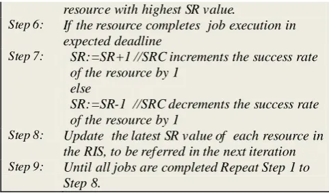
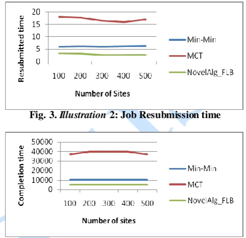
4.2. Illustration 2: Demand for computing resource is large and the amount of data transmission is large.

The available data transmission rate and CPU are the two important criterion that are looked at in this case. Since, VF takes into study many factors those sites that arrange resources that are stable will be first ones to be selected as shown in Fig. 3 & Fig. 4.

Fig. 3. Illustration 2: Job Resubmission time

Fig. 4. Illustration 2: Job completion time

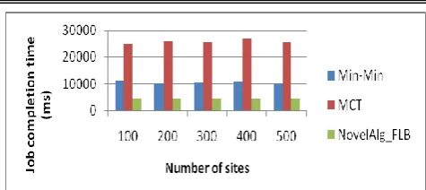
4.3. Illustration3: Demand for computing resource is large, and amount of data transmission is small The available CPU capacity and memory provided by the site will affect job completion in this case. Therefore, the site-transmission-rate impact on the completion time of the job is not significant. The experimental results obtained are shown in Fig. 5 & Fig. 6. These results indicate that the sites with largest CPU resource are first selected in MCT. However, Min– min, in contrast, first selects the combination with the site and job that consumes the shortest time thus making the completion time of required job shorter than MCT. However, Min– min does not consider the memory provided by the site. VF considers not only the CPU capacity, but also the memory, the transmission rate, past job completion rate and load of the site.

(9)

Fig. 6. Illustration3: Job completion time

4.4. Illustration 4: Demand for computing resource is small and the amount of data transmission is small.

The resources provided by a site do not have a significant impact in this case. In Fig. 7 & Fig 8, it is shown that MCT and Min-min only consider CPU capability, but the memory and transmission rate are not considered. The VF considers not a single factor but multiple factors, so a shorter time of completion is always required; this differs from most of the other alternative methods as shown in Fig. Hence this algorithm is more effective in balancing the load of the system.

Fig. 7. Illustration 4: Job Resubmission time

Fig. 8. Illustration 4: Job completion time

CONCLUSSION

Balanced job scheduling and load balancing is one issue that needs to be properly handled for the efficient working of a grid. The contributions of the algorithm mentioned above, NovelAlg_FLB include: (1) Passive replication does not appear in the earlier distributed load balancing algorithms. However, the proposed method devises a new fault tolerant load balancing algorithm that uses it.

(2) The messages that various resources of NovelAlg_FLB exchange among themselves are

simple and small in size thus preventing congestion in the network even when there is heavy traffic due to high arrival rates of jobs.

(3) This algorithm makes use of both static and dynamic load balancing policies to se lect the effective sites. (4) This algorithm implements simple computations. (5) Whenever any site becomes ineffective, this algorithm identifies the imbalance in the shortest time possible and also helps the grid to recover from the imbalance.

REFERENCES

[ASM04] Alomari R., Somani A. K., Manimaran G. - Efficient overloading techniques for primary-backup scheduling in realtime systems. Journal of Parallel and Distributed Computing 2004;64:629– 48.

[GMM97] Ghosh S., Melhem R., Mosse D. - Fault-tolerance through scheduling of aperiodic tasks in hard real-time multiprocessor systems. IEEE Trans Parallel and Distributed Systems 1997;8(3):272– 84.

[HK03] Hwang S., Kesselman C. - A flexible framework for fault tolerance in the Grid. Journal of Grid Computing 2003;1:251–72.

[JN12] Jasma Balasangameshwara,

Nedunchezhian Raju - A hybrid policy for fault tolerant load balancing in grid computing environments, Journal of Network and Computer Applications 35 (2012) 412– 422.

[JVS12] K. Jairam Naik, K. Vijay Kumar, N. Satyanarayana - Scheduling Tasks on Most Suitable Fault tolerant Resource for Execution in Computing Grid, IJGDC, Vol. 5, No. 3, Sep-2012, pp. 121–132.

(10)

Generation Computer Systems 2009;25:819– 28.

[LZ07] Lu Kai, Zo maya Albert Y. - A hybrid policy for job scheduling and load balancing in heterogeneous computational Grids. In: Sixth international symposium on parallel and distributed computing (ISPDC’07), 2007.

[Nae99] Naedele M. - Fault-tolerant real-time scheduling under execution time constraints. In: Proceedings of the sixth international conference on real-time multi-criteria scheduling 785 computing systems and applications, Hong Kong, China, December 13–16, p. 392. IEEE Computer Society, 1999.

[OS97] Oh Y., Son S. H. - Scheduling real-time tasks for dependability. Journal of Operational Research Society 1997;48(6):629–39.

[QJ06] Qin X., Jiang H. - A novel fault-tolerant scheduling algorithm for precedence constrained in real-time heterogeneous systems. Journal of Parallel Computing 2006;32:331– 46.

[Son94] Song J. - A partially asynchronous and iterative algorithm for distributed load balancing. Journal of Parallel Computing 1994;20(6):853–68.

[T+05] Tourino J., Martin M. J., Tarrio J., Arenaz M. - A Grid portal for an undergraduate parallel programming course. IEEE Transactions on Education 2005;48(3): 391–9.

[WR93] Willebeek-LeMair M. H., Reeves A. P.