https://doi.org/10.5194/gmd-11-4435-2018 © Author(s) 2018. This work is distributed under the Creative Commons Attribution 4.0 License.
Regional Climate Model Evaluation System powered by Apache
Open Climate Workbench v1.3.0: an enabling tool for
facilitating regional climate studies
Huikyo Lee1, Alexander Goodman1, Lewis McGibbney1, Duane E. Waliser1, Jinwon Kim2,3, Paul C. Loikith4, Peter B. Gibson1, and Elias C. Massoud1
1Jet Propulsion Laboratory, California Institute of Technology, Pasadena, CA, USA
2Joint Institute for Regional Earth System Science & Engineering, University of California, Los Angeles, CA, USA 3National Institute of Meteorological Sciences/Korean Meteorological Administration, Seogwipo, South Korea 4Department of Geography, Portland State University, Portland, OR, USA
Correspondence:Huikyo Lee ([email protected]) Received: 24 April 2018 – Discussion started: 18 June 2018
Revised: 5 October 2018 – Accepted: 11 October 2018 – Published: 5 November 2018
Abstract. The Regional Climate Model Evaluation System (RCMES) is an enabling tool of the National Aeronautics and Space Administration to support the United States National Climate Assessment. As a comprehensive system for evalu-ating climate models on regional and continental scales us-ing observational datasets from a variety of sources, RCMES is designed to yield information on the performance of cli-mate models and guide their improvement. Here, we present a user-oriented document describing the latest version of RCMES, its development process, and future plans for im-provements. The main objective of RCMES is to facilitate the climate model evaluation process at regional scales. RCMES provides a framework for performing systematic evaluations of climate simulations, such as those from the Coordinated Regional Climate Downscaling Experiment (CORDEX), us-ing in situ observations, as well as satellite and reanalysis data products. The main components of RCMES are (1) a database of observations widely used for climate model eval-uation, (2) various data loaders to import climate models and observations on local file systems and Earth System Grid Federation (ESGF) nodes, (3) a versatile processor to subset and regrid the loaded datasets, (4) performance met-rics designed to assess and quantify model skill, (5) plot-ting routines to visualize the performance metrics, (6) a toolkit for statistically downscaling climate model simula-tions, and (7) two installation packages to maximize con-venience of users without Python skills. RCMES website is maintained up to date with a brief explanation of these
components. Although there are other open-source software (OSS) toolkits that facilitate analysis and evaluation of cli-mate models, there is a need for clicli-mate scientists to partic-ipate in the development and customization of OSS to study regional climate change. To establish infrastructure and to ensure software sustainability, development of RCMES is an open, publicly accessible process enabled by leveraging the Apache Software Foundation’s OSS library, Apache Open Climate Workbench (OCW). The OCW software that pow-ers RCMES includes a Python OSS library for common cli-mate model evaluation tasks as well as a set of user-friendly interfaces for quickly configuring a model evaluation task. OCW also allows users to build their own climate data anal-ysis tools, such as the statistical downscaling toolkit provided as a part of RCMES.
Copyright statement. © 2018 California Institute of Technology. Government sponsorship acknowledged.
1 Introduction
meteoro-logical variables, exhibit considerable geographical variabil-ity. For example, warming is of a larger magnitude in the polar regions as compared with lower latitudes, due in part to a positive feedback related to rapidly receding polar ice caps (Gillett and Stott, 2009). This regional-scale variabil-ity makes it an extremely difficult task to accurately make projections of climate change, especially on a regional scale. Yet, characterizing present climate conditions and providing future climate projections at a regional scale are far more use-ful for supporting decisions and management plans intended to address impacts of climate change than global-scale cli-mate change information.
Regional climate assessments heavily depend on numeri-cal model projections of future climate simulated under en-hanced greenhouse emissions that not only provide predic-tions of physical indicators but also indirectly inform on so-cietal impacts, thus providing key resource for addressing adaptation and mitigation questions. These quantitative pro-jections are based on global and regional climate models (GCMs and RCMs, respectively). Due to the critical input such models have for decision makers, it is a high priority to make them subject to as much observational scrutiny as possible. This requires the systematic application of observa-tions, in the form of performance metrics and physical pro-cess diagnostics, from gridded satellite and reanalysis prod-ucts as well as in situ station networks. These observations then provide the target for model simulations, with confi-dence in model credibility boosted where models are able to reproduce the observed climate with reasonable fidelity. Enabling such observation-based multivariate evaluation is needed for advancing model fidelity, performing quantita-tive model comparison, evaluation and uncertainty analyses, and judiciously constructing multi-model ensemble projec-tions. These capabilities are all necessary to provide a reli-able characterization of future climate that can lead to in-formed decision-making tailored to the characteristics of a given region’s climate.
The Coupled Model Intercomparison Project (CMIP), currently in its sixth phase, is an internationally coordi-nated multi-GCM experiment that has been undertaken for decades to assess global-scale climate change. The Coordi-nated Regional Downscaling Experiment (CORDEX; Giorgi and Gutowski, 2015; Gutowski Jr. et al., 2016) is another modeling effort that parallels CMIP but with a focus on regional-scale climate change. To complement CMIP, which is based on GCM simulations at relatively coarse resolu-tions, CORDEX aims to improve our understanding of cli-mate variability and changes at regional scales by providing higher-resolution RCM simulations for 14 domains around the world. Climate scientists analyze the datasets from CMIP and CORDEX, with the findings contributing to the Inter-governmental Panel on Climate Change (IPCC) assessment reports (e.g., IPCC, 2013). Plans and implementation for the CMIP6 (Eyring et al., 2016a) are now underway to feed into the next IPCC assessment report (AR6; IPCC, 2018). In
coor-dination with the IPCC efforts, the Earth System Grid Feder-ation (ESGF) already hosts a massive amount of GCM output for past CMIPs, with CMIP6 and RCM output for CORDEX slated for hosting by ESGF as well. Due to the large variabil-ity across the models that contribute to CMIP, it is a high pri-ority to evaluate the models systematically against observa-tional data, particularly from Earth remote sensing satellites (e.g., Teixeira et al., 2014; Freedman et al., 2014; Stanfield et al., 2014; Dolinar et al., 2015; Yuan and Quiring, 2017). As more GCMs and RCMs participate in the two projects, the ESGF infrastructure faces a challenge of providing a com-mon framework where users can analyze and evaluate the models using the observational datasets hosted on the ESGF, such as the observations for Model Intercomparison Projects (obs4MIPs; Ferraro et al., 2015; Teixeira et al., 2014) and reanalysis data (ana4MIPs; ana4MIPs, 2018).
As careful and systematic model evaluation is widely rec-ognized as critical to improving our understanding of future climate change, there have been other efforts to facilitate this type of study. Here, we briefly describing existing model evaluation toolkits for CMIP GCMs. The Community Data Analysis Tools (CDAT; LLNL, 2018) is a suite of software that enables climate researchers to solve their data analysis and visualization challenges. CDAT has already successfully supported climate model evaluation activities for the United States Department of Energy (DOE)’s climate applications and projects (DOE, 2018), such as the IPCC AR5 and Ac-celerated Climate Modeling for Energy. The Earth System Model Evaluation Tool (ESMValTool; Eyring et al., 2016b; Lauer et al., 2017) is another software package that offers a variety of tools to evaluate the CMIP GCMs. The diag-nostic tools included in ESMValTool are useful not only for assessing errors in climate simulations but also provid-ing better understandprovid-ing of important processes related to the errors. While ESMValTool has facilitated global-scale assessments of the CMIP-participating GCMs, the devel-opment and application of infrastructure for a systematic, observation-based evaluation of regional climate variability and change in RCMs are relatively immature, owing in con-siderable part to the lack of a software development platform to support climate scientist users around the world.
Therefore, it is crucial to leverage the added value of RCMs, because they will improve our estimation of the re-gional impacts of climate change. RCM experiments, such as CORDEX, will play a critical role in providing finer-scale climate simulations. This role also fits the US National Cli-mate Assessment’s (NCA; Jacobs, 2016) strategic objective, to produce a quantitative national assessment with consid-eration of uncertainty. Here, assessment of the uncertainty in simulated climate requires comprehensive evaluation of many RCMs against in situ and remote sensing observations and regional reanalysis data products. The observation-based evaluation of multiple RCMs with relatively high resolution also requires the appropriate architectural framework capable of manipulating large datasets for specific regions of interest. Recognizing the need for an evaluation framework for high-resolution climate models with a special emphasis on regional scales, the Jet Propulsion Laboratory (JPL) and the Joint Institute for Regional Earth System Science and Engi-neering (JIFRESSE) at the University of California, Los An-geles (UCLA), have developed a comprehensive suite of soft-ware resources to standardize and streamline the process of interacting with observational data and climate model output to conduct climate model evaluations. The Regional Climate Model Evaluation System (RCMES; JPL, 2018a; Mattmann et al., 2014; Whitehall et al., 2012) is designed to provide a complete start-to-finish workflow to evaluate multi-scale climate models using observational data from the RCMES database and other data sources including the ESGF (e.g., obs4MIPs) and JPL’s Physical Oceanographic Data Active Archive Center (PO.DAAC; JPL, 2018c).
RCMES is mutually complementary to CDAT and ESM-ValTool with the main target of supporting CORDEX and NCA communities by fostering the collaboration of climate scientists in studying climate change at regional scales. To promote greater collaboration and participation of the cli-mate research community within the RCMES development process, we transitioned from a closed-source development process to an open-source software (OSS) community-driven project hosted in the public forum. As a result, the devel-opment process is subject to public peer review, something which has significantly improved the overall project quality. RCMES is Python-based OSS powered by the Apache Soft-ware Foundation’s (ASF) Open Climate Workbench (OCW) project. OCW is a Python library for common model eval-uation tasks (e.g., data loader, subsetting, regridding, and performance metrics calculation) as well as a set of user-friendly interfaces for quickly configuring a large-scale re-gional model evaluation task. OCW acts as the baseline in-frastructure of RCMES, allowing users to build their own cli-mate data analysis tools and workflows.
The primary goal of this paper is to document RCMES as powered by OCW, as well as to describe the workflow of evaluating RCMs against observations using RCMES. Re-cent developments on the workflow include a template for performing systematic evaluations of CORDEX simulations
for multiple variables and domains. We also demonstrate the benefits of developing RCMES in a collaborative manner by leveraging ASF’s OCW project. Experience tells us that there is strong demand for peer-reviewed documentation in sup-port of RCMES used by climate scientists, and this paper provides exactly that.
The paper is organized as follows. Section 2 describes the overall software architecture of RCMES, followed by de-tailed description on each component of RCMES in Sect. 3. Section 4 presents the value of developing OSS within a pub-lic community-driven model. Section 5 provides summary and future development plans.
2 Overall structure of RCMES
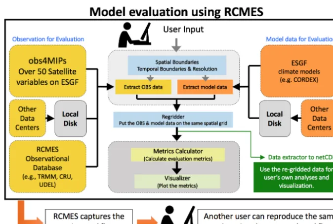
RCMES provides datasets and tools to assess the quantitative strengths and weakness of climate models, typically under present climate conditions for which we have observations for comparison, which then forms a basis to quantify our understanding of model uncertainties in future projections. The system and workflow of RCMES are schematically illus-trated in Fig. 1. There are two main components of RCMES. The first is a database of observations, and the second is the RCMES toolkits. The workflow of climate model evaluation implemented by RCMES starts with loading observation and model data. Currently, RCMES users can load datasets from three different sources: (1) RCMES database, (2) local stor-age, (3) ESGF servers (e.g., obs4MIPs), and any combina-tions of (1)–(3). Access to other datasets archived on remote servers will be tested and implemented in future versions. Once the datasets are loaded, RCMES subsets the datasets spatially and temporally, and optionally regrids the subsetted datasets, compares the regridded datasets, calculates model performance metrics, and visualizes/plots the metrics. The processed observational and model datasets are saved in a NetCDF file. All of this model evaluation process is con-trolled by user input. Because RCMES captures the entire workflow, another user can reproduce the same results using the captured workflow.
Figure 2 displays the step-by-step pathway for learning and using RCMES. As an introduction to RCMES, the sim-ple but intuitive command-line interface (CLI) is provided. Running RCMES using a configuration file (CFile) enables a basic but important and comprehensive evaluation of multi-ple climate models using observations from various sources. Advanced users can utilize the OCW library to write scripts for customized data analysis and model evaluation.
Figure 1.The outline and data flows within RCMES (adapted from JPL, 2018a).
Figure 2.The approach to getting acquainted and using RCMES and OCW (adapted from JPL, 2018a).
each step of the RCM evaluation. Although the model evalu-ation through CLI is limited to calculating climatological bi-ases of one RCM simulation against one of the observational datasets from the RCMES database, the CLI offers RCMES users an opportunity to learn the basic process of model eval-uation, which includes inputting model datasets and obser-vations, specifying gridding options, calculating the model’s bias, and plotting the results.
CFiles lie at the heart of RCMES to support user-customized evaluation of multiple RCMs, such as those par-ticipating in CORDEX, and their ensemble means. To max-imize their utility, RCMES CFiles use the Python YAML (YAML Ain’t Markup Language) format of namelist files that are familiar to many climate scientists who run climate models. CFiles include a complete start-to-finish workflow of model evaluation as shown in Fig. 4. In CFiles, users
Figure 3.The four steps of model evaluation included as a CLI example of RCMES.
Figure 4.The process of evaluating climate models using datasets from multiple sources and modularized OCW libraries. The evaluation metrics and plots in Kim et al. (2013) are shown as an example.
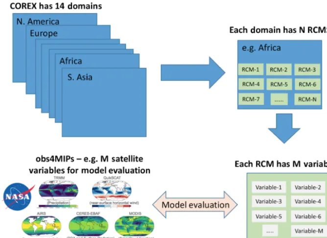
Figure 5 illustrates the latest RCMES development to pro-vide an easy solution to evaluate key variables simulated by CORDEX RCMs against satellite observational datasets from obs4MIPs. Currently, running RCMES with a CFile en-ables evaluation of multiple models for one variable over a specified domain. Given more than 30 different obs4MIPs variables, RCMES provides a script named “cordex.py” to generate configuration files automatically. Users are re-quested to select one of the 14 CORDEX domains and pro-vide a directory path on a local machine where obs4MIPs and model datasets are archived. Then, the script extracts vari-able and CORDEX domain information from searched file names in subdirectories of the given directory path by utiliz-ing the climate and forecast (CF) namutiliz-ing convention (Meta-Data, 2018) for the obs4MIPs and CORDEX data files avail-able from ESGF servers. The RCMES website also provides these examples of the multi-model, multi-variable evaluation for several CORDEX domains (North America, Europe, and Africa) as a part of the RCMES tutorial. As an example, run-ning RCMES for CORDEX North America domain with 12 variables and three seasons (36 unique evaluations with five datasets each) takes about 45 min using an Intel Xeon CPU with a clock rate of 2.30 GHz on a multi-core GNU/Linux computing platform.
Continuously reflecting climate scientists’ needs and fa-cilitating greater scientific yield from model and observa-tion datasets are important for expanding the future user base of RCMES. Despite the development environment encour-aging participation of open communities, one of the main
challenges in using RCMES for evaluating climate models has been to support dataset files in various formats. To ad-dress this issue, the development of flexible and versatile data loaders that read files with different formats is required. An-other limiting factor of the CFile-based format utilized by RCMES is that it is not easy to calculate sophisticated di-agnostics with which the model evaluation process does not fit into the workflow in Fig. 4. Most of the model evaluation metrics included in the current RCMES distribution are intu-itive but relatively rudimentary, such as a bias, a root mean square error, and linear regression coefficients. Although cli-mate scientists obtain an insight into clicli-mate models with these basic metrics calculated and visualized with RCMES, model assessments and, ultimately, future model improve-ment require more comprehensive and mathematically rigor-ous metrics for quantifying models’ uncertainty.
program-ming language. It is also possible to mix OCW file load-ers and processors with other Python libraries. The tutorial page on the RCMES website also describes various applica-tions of using OCW modules for advanced analyses of cli-mate science data. For instance, Kim et al. (2018) and Lee et al. (2017) use RCMES to compare the high-resolution sim-ulations made using NASA Unified Weather Research and Forecasting model (Peters-Lidard et al., 2015) with daily and hourly observations. The tutorials on the RCMES website explain how to reproduce figures included in these published articles.
3 Components of RCMES
In the following, we describe seven software components of RCMES: (1) data loader (Sect. 3.1), (2) the RCMES database (Sect. 3.1.1), (3) dataset processor (Sect. 3.2), (4) metrics and (5) plotter (Sect. 3.3), (6) statistical downscaling mod-ule (Sect. 3.4), and (7) installation package options for dis-seminating RCMES (Sect. 3.5). Our website (JPL, 2018a), updated with new developments and examples on a regular basis, is also a vital component of RCMES. As illustrated in Fig. 4, climate model evaluation using RCMES starts with loading observation and model data using OCW. The obser-vation data can be pulled from different sources. The main function of the dataset processor is to subset and regrid the dataset objects. The dataset processor also saves the pro-cessed datasets in a user-specified NetCDF file. Since indi-vidual modules in the data loader and dataset processor can be used and combined for various purposes, we provide a user-friendly manual in the current paper describing the mod-ules.
3.1 Data loader
The first step in performing any climate model evaluation is determining which observational and model datasets to use and retrieving them for subsequent use. Ideally, one would like to support a standardized, user-friendly interface for data retrieval from the most common sources used by cli-mate scientists. OCW facilitates this by providing RCMES with several dataset loaders to read and write CF-compliant NetCDF files, and loaders for specific datasets. The objec-tive of offering some specific loaders, such as loaders for the Weather Research and Forecasting (WRF; Skamarock et al., 2008) model’s raw output or the Global Precipitation Mea-surement (GPM; Huffman et al., 2015) observation data, is to expand the convenience of users’ customized model eval-uation studies using observation and model data files from various sources without file conversion. By design, all of the dataset loaders return a dataset object or a list of multi-ple dataset objects which store gridded variables with arrays of latitudes, longitudes, times, and variable units regardless of the format of the original data files. When handling
in-put gridded data in three spatial dimensions with elevation, users need to specify elevation_index, an optional parameter of dataset loaders. By default, elevation_index is zero. The following subsections describe four data sources for which RCMES has built-in support.
3.1.1 RCMES database (RCMED)
RCMES is a comprehensive system whose distribution in-cludes its own database of observational datasets that can be readily accessed for evaluating climate models. Currently, the database provides 14 datasets from ground stations and satellites to support basic model evaluation. Among those, precipitation data from NASA’s Tropical Rainfall Measur-ing Mission (TRMM; Huffman et al., 2007), temperature, and precipitation data from the CRU (Harris et al., 2014) are widely used by the climate science community. The RCMES database (RCMED) also provides evaporation, precipitation, and snow water equivalent datasets from NASA’s reanalysis products. The RCMED loader requires the following param-eters:
– dataset_id, parameter_id: identifiers for the dataset and variable of interest (https://rcmes.jpl.nasa.gov/content/ data-rcmes-database, last access: 26 October 2018); and
– min_lat, max_lat, min_lon, max_lon, start_time, end_time: spatial and temporal boundaries used to subset the dataset domain.
From an implementation perspective, these parameters are used to format a representational state transfer (REST) query which is then used to search the RCMED server for the re-quested data. The loaders provided by OCW for two of the other data sources (ESGF and PO.DAAC) also work in a sim-ilar fashion.
3.1.2 Local filesystem
The simplest and most standard way to access Earth sci-ence datasets is storing NetCDF files in the local filesys-tem. The ocw.data_source.local module reads, modifies, and writes to the locally stored files. In addition to loading one dataset object from one file, this module also contains load-ers for loading a single dataset spread across multiple files, as well as multiple datasets from multiple files. In each case, dataset variables and NetCDF attributes are extracted into OCW datasets using the NetCDF4 or hdf5 Python libraries. Most of the remote data sources described in the next few sessions also depend on these loaders, since they generally entail downloading datasets to the local filesystem as the first step, then loading them as locally stored files. The following parameters are required to load one file:
Figure 5.The multi-model, multi-variable evaluation against satellite observations from obs4MIPs over the 14 CORDEX domains.
– variable_name: the name of the variable to load, as is defined in the NetCDF file.
By default, the local loader reads the spatial and tempo-ral variables (latitude, longitude, and time) by assuming they are commonly used variable names (e.g., lat, lats, or lati-tude), which should typically be the case if the file to be loaded is CF-compliant. However, these variable names can be manually provided to the loader for files with more un-usual naming conventions for these variables. In the loader, these parameters are, respectively, lat_name, lon_name, and time_name.
3.1.3 Earth System Grid Federation (ESGF)
The Earth System Grid Federation (ESGF), led by Program for Climate Model Diagnosis and Intercomparison (PCMDI) at the Lawrence Livermore National Laboratory (LLNL) (Taylor et al., 2012), provides CF-compliant climate datasets for a wide variety of projects including CMIP, obs4MIPS, and CORDEX. Provided that the user can authenticate with a registered account (via OpenID), data can be readily ac-cessed through a formatted search query in a similar manner to the PO.DAAC and RCMED data sources as the first step of model evaluation using RCMES. The ESGF loader requires the following parameters:
– dataset_id: identifier for the dataset on ESGF;
– variable_name: the name of the variable to select from the dataset, in CF short name form; and
– esgf_username, esgf_password: ESGF username (e.g., OpenID) and password used to authenticate.
ESGF provides its data across different nodes which are maintained by a variety of climate research and modeling in-stitutes throughout the world. The loader searches the JPL node by default, which contains CMIP5 and obs4MIPS data. However, if datasets from other projects are desired, then the base search URL must also be specified in the loader via the search_url parameter. For example, the Deutsches Klimarechenzentrum (DKRZ) node (search_url=https://esgf-data.dkrz.de/esg-search/search) should be used if the user wishes to obtain CORDEX model output.
3.1.4 NASA’s Physical Oceanographic Data Active Archive Center (PO.DAAC)
level-4 blended datasets covering a myriad of gridded spatial res-olutions between 0.05 and 0.25◦, a range of temporal
resolu-tions from daily to monthly, parameters (gravity, glaciers, ice sheets, ocean circulation, ocean temperature, etc.), latencies (near-real time, delayed mode, and non-active), collections (Cross-Calibrated Multi-Platform Ocean Surface Wind Vec-tor Analysis Fields, Climate Data Record, Group for High Resolution Sea Surface Temperature (GHRSST), etc.), plat-forms (ADEOS-II, AQUA, AQUARIUS_SAC-D, Coriolis, DMSP-F08, etc.), sensors (AATSR, AHI, AMR, AMSR-E, AMSR2, AQUARIUS_RADIOMETER, etc.), spatial cover-ages (Antarctica, Atlantic and Pacific, Baltic Sea, Eastern Pa-cific Ocean, global, etc.), and data formats (ASCII, NetCDF, and RAW).
As all data loaded by RCMES loaders generate dataset objects with spatial grid information, currently only level-4 blended PO.DAAC datasets are suitable for evaluat-ing climate models usevaluat-ing RCMES. To synchronize the dataset search and selection, the PO.DAAC loader pro-vides a convenience utility function which returns an up-to-date list of available level-4 granule dataset IDs which can be used in the granule extraction process. Once the list_available_level4_extract_granule_dataset_ids() function has been executed and a suitable dataset_id selected from the returned list, the PO.DAAC loader can be invoked with the following granule subset and granule download functions.
subset_granule:
– variable: the name of the variable to read from the dataset;
– name=”: (optional) a name for the loaded dataset; – path=’/tmp’: (optional) a path on the filesystem to store
the granule; and
– input_file_path=”: a path to a JSON file which contains the subset request that you want to send to PO.DAAC. The JSON syntax is explained at https://podaac.jpl.nasa. gov/ws/subset/granule/index.html (last access: 26 Octo-ber 2018).
extract_l4_granule:
– variable: the name of the variable to read from the dataset;
– dataset_id=”: dataset persistent ID (the ID is required for a granule search), e.g., PODAAC-CCF35-01AD5; – name=”: (optional) a name for the loaded dataset; and – path=’/tmp’: a path on the filesystem to store the
gran-ule.
3.2 Dataset processor
Once the data are loaded, the next step is to homogenize the observational and model datasets such that they can be com-pared with one another. This step is necessary because, in
many cases, the input datasets can vary in both spatial and temporal resolution, domain, and even physical units. Op-erations for performing this processing step on individual OCW datasets can be found in the dataset_processor mod-ule, which will be described in greater detail in the following subsections. All of these data processing tools make use of the NumPy and SciPy libraries (van der Walt et al., 2011) of Python.
3.2.1 Subsetting
The first processing step is subsetting, both in space and time. This is especially important for evaluating RCMs since many observational datasets are defined on global grids, so a sim-ple subset operation can greatly reduce the potential mem-ory burden. The following parameters are required for sub-setting:
– subregion: the target domain. This includes spatial and temporal bounds information, and can be derived from a rectangular bounding box (lat–long pairs for each cor-ner), one of the 14 CORDEX domain names (e.g., North America), or a mask matching the dimensions of the in-put dataset.
For clearer tractability, a subregion_name parameter can be provided to label the domain. If the user wishes to subset the data further based on a matching value criterion, these may be provided as a list via the user_mask_values param-eter. Finally, the extract parameter can be toggled to control whether or not the subset is extracted (e.g., the output di-mensions conform to the given domain) or not (the original dimensions of the input dataset are preserved, and values out-side the domain are masked).
A temporal (or rather seasonal) subset operation is also supported. The parameters are
– month_start, month_end: start and end months which denote a continuous season. Continuous seasons which cross over new years are supported (e.g., (12, 2) for DJF).
The average_each_year parameter may be provided to av-erage the input data along the season in each year.
3.2.2 Temporal resampling and spatial regridding Having addressed inhomogeneities in the input datasets with respect to domain, discrepancies in spatial and temporal res-olution need to be considered. Resampling data to a lower temporal resolution (e.g., from monthly to annually) is per-formed via a simple arithmetic mean and requires the follow-ing parameter:
Spatial regridding, on the other hand, is the most computa-tionally expensive operation. OCW provides a relatively ba-sic implementation which utilizes SciPy’s “griddata” func-tion for bilinear interpolafunc-tion of 2-D fields. The parameters required by the user are
– new_latitudes, new_longitudes: one- or two-dimensional arrays of latitude and longitude values which define the grid points of the output grid.
3.2.3 Unit conversion
Because physical variables can be expressed in a large vari-ety of units, RCMES supports automatic unit conversion for a limited subset of units. These include conversion of all tem-perature units into Kelvin and precipitation into mm day−1. 3.3 Metrics and plotter
The current RCMES distribution offers various model evalu-ation metrics from ocw.metrics. There are two different types of metrics. RCMES provides basic metrics, such as bias cal-culation, Taylor diagram, and comparison of time series. Ear-lier RCMES publications (Kim et al., 2013, 2014) show how to use the basic metrics in multi-model evaluation as illus-trated in Fig. 4. The metrics module also provides more ad-vanced metrics. For example, a joint histogram of precipita-tion intensity and duraprecipita-tion (Kendon et al., 2014; Lee et al., 2017) can be calculated using hourly precipitation data from observations or model simulations. The joint histogram can be built for any pairs of two different variables as well. An-other set of metrics that have been recently added enables evaluation of long-term trends in climate models over the contiguous United States and analysis of the associated un-certainty.
The final step in any model evaluation is visualizing cal-culated metrics. For this purpose, OCW includes some utili-ties for quickly generating basic plots which make use of the popular matplotlib plotting package (Hunter, 2007). These include time series, contour maps, portrait diagrams, bar graphs, and Taylor diagrams. All of the included plotting rou-tines support automatic subplot layout, which is particularly useful when RCMES users evaluate a large number of mod-els altogether.
3.4 Statistical downscaling using RCMES
As stated in the introduction, the spatial resolution of GCMs is typically coarse relative to RCMs due to the high com-putational expense of GCMs. To use output from GCM simulations for studying regional climate and assessing im-pacts, GCM simulations typically need to be downscaled, a process that generates higher-resolution climate information from lower-resolution datasets. Although RCMs provide a physics-driven way to dynamically downscale GCM simula-tions, the computational expense of running RCMs can be
substantial. In addition, it is sometimes necessary to correct the errors in the simulated climate that deviate from observa-tions.
Recognizing the needs for downscaling and error correc-tion, RCMES provides a toolkit for statistically downscaling simulation output from CMIP GCMs and correcting the out-put for present and future climate. The statistical downscal-ing toolkit supports different methods adapted from previ-ous studies including a simple bias correction, bias correc-tion and spatial disaggregacorrec-tion, quantile mapping, and asyn-chronous regression approach (Stoner et al., 2013). All of these simple statistical downscaling approaches are intuitive and easy to understand.
The statistical downscaling script accepts users’ input from a CFile. This CFile is somewhat different from one for model evaluation using RCMES but uses the same YAML format. The input parameters include a geographical location of the point to downscale GCM output, temporal range, and source of observational and model datasets. Users can select one of observations from RCMED (Sect. 4.1.1) or local file system (Sect. 4.1.2). GCM output needs to be stored in the local file system. The statistical downscaling generates (1) a map file, (2) histograms, and (3) a spreadsheet. The map and histogram are portable graphics format (PNG) files, and the spreadsheet file has the Excel spreadsheet (XLS) extension. The map shows a location of downscaling target specified in the CFile. The histograms using numbers in the spreadsheet show distributions of the observation and the original and downscaled model datasets. The RCMES tutorial explains the entire process of statistical downscaling in great detail.
3.5 Download and installation of RCMES
There are two ways to download and install RCMES. One is executing a one-line command to install one of the RCMES packages using the terminal application. The other is with a virtual machine (VM) environment. RCMES execution with the latter is slower than the package installation, but it pro-vides Linux OS and all required Python libraries that can run on any type of users’ computers.
3.5.1 Installation package
3.5.2 Virtual machine image
For novice users who are not familiar with Unix and Linux terminals, there is an option to run RCMES without the pack-age installation. As a completely self-contained research en-vironment running with VirtualBox (Oracle, 2018), the VM approach offers a plug and play approach that enables users to quickly begin exploring RCMES without any trouble in the installation process. The RCMES VM image contains Linux, Python 2.7, OCW libraries, dependencies, and data analysis examples, as well as the latest version of sample datasets to execute some tutorials.
The VM image is an implementation of the same com-puting environment as the OCW developers with users’ own computers. Several RCMES training sessions have utilized the VM image as a means for sharing RCMES source codes and generating the tutorial examples with user-specific cus-tomization. As an additional benefit, when a user no longer requires the VM image, the image can be easily replaced or completely removed from the host environment without af-fecting other software or libraries that may be installed.
4 Community software development
In the early development phase of RCMES, we encountered climate scientists from around the world who have the de-sire to publish their source codes for climate data analysis and model evaluation, proactively contributing to the OSS, and have their code made available as official software re-leases with appropriate licenses constraining reuse of their software. To encourage the potential benefit of collaborative development of OSS, the RCMES team decided to transi-tion the development process from a closed-source project at JPL to an open-source, community-driven project hosted by ASF (ASF, 2018a) in 2013. The goal of this transition was to not only make the RCMES codebase readily available under a permissive license, e.g., the Apache Licence v2.0 (ASF, 2018c), but also to focus on growing this sustainable and healthy environment, named as OCW. Any climate scientist can make contributions to OCW that comprises RCMES. At this time, the opinion was that, without an active and pas-sionate community, RCMES would become of lesser value to everyone. Hence, the OCW project mantra has always followed a “community over code” model. This aspiration would eventually result in OCW becoming the second ever JPL-led project to formally enter incubation at the ASF, fur-ther establishing JPL as a leader in well-governed, sustain-able, and successful transition of government-funded soft-ware artifacts to the highly recognized and renowned ASF, where the primary goal is to provide software for the public good. Having undertaken an incubation period (ASF, 2018b) of about 18 months, OCW successfully graduated from the Apache Incubator in March 2014, with the result being that OCW could stand alongside 100 top-level software projects
all governed and developed under the iconic Apache brand. Since entering incubation, the OCW Project Management Committee (PMC) has developed, managed and successfully undertaken no fewer than nine official Apache releases, a process involving stringent review by the extensive, globally distributed Apache community (some 620 individual mem-bers, 5500 code committers, and thousands of contributors). In addition, OCW has been presented in countless confer-ences since its first release in June 2013.
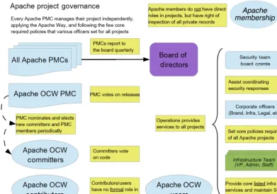
From the outset, the OCW project development has fol-lowed a well-established, structured, and independently man-aged community development process where a governing body, referred to as the OCW PMC, is responsible for the proper management and oversight of OCW, voting on soft-ware product releases and electing new PMC members and committers to the project. As well as deciding upon and guid-ing the project direction, the OCW PMC reports directly to the ASF board of directors on a quarterly basis, providing up-dates on community and project specifics such as community activity, project health, and any concerns, latest release(s) ad-ditions to the PMC, etc. Figure 6 provides an overview of the project governance also providing additional context as to where and how OCW fits into the foundational structure of the ASF.
OCW follows a review-then-commit source code review process, where new source code contributions from any party are reviewed by typically more than one OCW commit-ter who has write permissions for the OCW source code. The OCW community uses several tools which enable the project and community to function effectively and grow. These include tailored instances of software project manage-ment tools such as
– Wiki documentation; confluence wiki software enabling the community to provide documentation for release procedures, functionality, software development pro-cess, etc.;
– source code management; the canonical OCW source code is hosted by the ASF in Git, with a public syn-chronized mirror provided at https://github.com/apache/ climate (last access: 26 October 2018);
– issue tracking; OCW committers use the popular JIRA issue tracking software for tracking development in-cluding bug fixes, new features and improvements, de-velopment drives and release planning;
– build management and continuous integration; both Jenkins and TravisCI provide nightly builds and pull re-quest continuous integration test functionality, respec-tively, ensuring that the OCW test suite passes and that regressions are mitigated between releases; and – project website; the primary resource for OCW is the
Figure 6.Schematic representation of Apache OCW project governance.
(last access: 26 October 2018). This is hosted by the ASF and maintained by the OCW PMC.
Using the tools listed above, OCW and the accompany-ing RCMES have been released by a release manager who is also a committer and PMC member with write access to the OCW source code. OCW release candidates follow strict peer review, meaning that they are official Apache releases (e.g., those which have been endorsed as an act of the foun-dation by the OCW PMC). The OCW PMC must obey the ASF requirements on approving any release meaning that a community voting process needs to take place before any OCW release can officially be made. For a release vote to pass, a minimum of three positive votes and more positive than negative votes must be cast by the OCW community. Releases may not be vetoed. Votes cast by PMC members are binding. Before casting+1 binding votes, individuals are required to download all signed source code packages onto their own hardware, verify that they meet all requirements of ASF policy on releases, validate all cryptographic signa-tures, compile as provided, and test the result on their own platform. A release manager should ensure that the commu-nity has a 72 h window of opportucommu-nity to review the release candidate before resolving or canceling the release process.
All of the OCW source codes and RCMES are freely avail-able under the Apache License v2.0 which is not only a re-quirement for all Apache projects but also desired by the OCW community due to the core project goals of open, free
use of high-quality OSS. Over time, we have witnessed a significant degree of community growth through availabil-ity of OCW through an open, permissive license such as the Apache License v2.0.
5 Summary and future development plans
Although there are other open-source software toolkits that facilitate analysis and evaluation of climate models, there is a need for climate scientists to participate in the develop-ment and customization of software to study regional climate change. To meet the need, RCMES provides tools to ana-lyze and document the quantitative strengths and weakness of climate models to quantify and improve our understand-ing of uncertainties in future predictions. The model evalua-tion using RCMES includes loading observaevalua-tional and model datasets from various sources, a processing step to collocate the models and observations for comparison, and steps to perform analysis and visualization.
facilitating informed decisions regarding climate change at a regional scale.
The present version of RCMES is populated with a num-ber of contemporary climate and regionally relevant satel-lite, reanalysis, and in situ based datasets, with the ability to ingest additional datasets of wide variety of forms, ingest climate simulations, apply a number of useful model perfor-mance metrics, and visualize the results. However, at present, the regridding routines included in the RCMES distribution are rudimentary, such as bilinear and cubic spline interpo-lation. Therefore, our future RCMES development will pri-oritize advancing the regridding scheme in OCW’s dataset processor including a tool for remapping datasets with dif-ferent spatial resolutions into the hierarchical equal area iso-latitude pixelization (HEALPix; Gorski et al., 2005) grids. HEALPix is an open-source library for fast and robust multi-resolution analysis of observational and model datasets re-gridded into HEALPix pixels, which have been widely used by astronomers and planetary scientists.
Future RCMES development will also include new met-rics for the calculation and interrogation of rainfall extremes in in situ observations, satellite, and regional climate model simulations. These will include a suite of precipitation met-rics based on the Expert Team on Climate Change Detection and Indices (ETCCDI; Zhang et al., 2011) and meteorologi-cal drought indices such as the standardized precipitation in-dex (SPI) and standardized precipitation evapotranspiration index (SPEI). Compound extreme events, known to carry dis-proportionate societal and economic costs, will also be a fo-cus. Examples of compound extreme events under consid-eration include heat stress (extreme temperature and humid-ity), wildfire conditions (extreme temperature and wind), and infrastructure damage (extreme rainfall and wind). We note that very few studies have comprehensively evaluated com-pound extreme events in regional climate model ensembles to date. Moving beyond the simple summary/descriptive statis-tics of model evaluation is also a priority, with the intention to include more process-oriented diagnostics of model bi-ases. Examples include investigating why some models sim-ulate extremes poorly as related to biases in surface turbu-lent fluxes in the land surface model component (Kala et al., 2016; Ukkola et al., 2018) or biases in large-scale atmo-spheric conditions (e.g., blocking) that can promote the onset of extreme events (Gibson et al., 2016).
Additionally, future work for RCMES will include the out-put of Bayesian metrics (or probabilistic metrics), such as those obtained by Bayesian model averaging (BMA; Raftery et al., 2005) or approximate Bayesian computation (ABC; Turner and Van Zandt, 2012). BMA can directly provide an inter-model comparison by diagnosing the various models’ abilities to mimic the observed data. Then a weight, with as-sociated uncertainty, is assigned to each model based on its comparison to the observations, where higher weights indi-cate more trustworthy models. Using an optimal combination of these weights, a more informed forecast/projection of the
climate system can be made, which can potentially provide more accurate estimates of the impact on regional systems. Unfortunately, BMA utilizes a likelihood (or cost) function when determining the model weights, which can sometimes be a roadblock for problems of high dimensions. Therefore, specified summary metrics can be defined for the problem, such as those related to extremes in precipitation or drought, and by using the ABC method we can replace the likelihood function needed for BMA with a cost function that minimizes only the difference between the observed and simulated met-rics rather than differences between the entirety of the data. This likelihood-free type of estimation is attractive as it al-lows the user to disentangle information in a time or space domain and use it in a domain that may be more suitable for the regional analysis (e.g., fitting the distribution of winter-time extreme precipitation or summerwinter-time extreme temper-ature as possible metrics). By combining BMA with ABC (Vrugt and Sadegh, 2013; Sadegh and Vrugt, 2014), a diag-nostic based approach for averaging regional climate models will be possible.
The information technology component of RCMES will also have enhanced parallel processing capabilities. Our fu-ture development of the OCW dataset processor will lever-age the maturity and capabilities of open-source libraries to facilitate the handling and distribution of massive datasets using parallel computing. Given the sizes of the multi-year model runs and observations at high spatial and temporal resolutions (kilometer and sub-hourly), scaling across a par-allel computing cluster is needed to efficiently execute the analysis of fine-scale features. SciSpark is a parallel ana-lytical engine for science data that uses the highly scalable MapReduce computing paradigm for in-memory computing on a cluster. SciSpark has been successfully applied to test-ing several RCMES use cases, such as mesoscale convective system (MCS) characterization (Whitehall et al., 2015) and the probability density function clustering of surface temper-ature (Loikith et al., 2013). We will apply and test SciSpark to analyses of high-resolution datasets and publish new ver-sions of RCMES with parallel-capable examples.
Lastly, the development of RCMES aims to contribute to the CORDEX community and US NCA in order to enhance the visibility and utilization of NASA satellite observations in the community.
Code and data availability. See Sect. 3.5 “Download and installa-tion of RCMES”.
Competing interests. The authors declare that we have no signif-icant competing financial, professional, or personal interests that might have influenced the performance or presentation of the work described in this paper.
Acknowledgements. The JPL authors’ contribution to this work was performed at the Jet Propulsion Laboratory, California Institute of Technology, under a contract with NASA. We thank NASA for supporting the RCMES project and US NCA. We acknowledge the Coordinated Regional Climate Downscaling Experiment under the auspices of the World Climate Research Programme’s Working Group on Regional Climate. We would like to express our appreciation to William Gutowski and Linda Mearns for coordinating the overall CORDEX program and CORDEX North America, respectively.
Edited by: Juan Antonio Añel
Reviewed by: Neil Massey and two anonymous referees
References
ana4MIPs: Reanalysis for MIPs, available at: https://esgf.nccs.nasa. gov/projects/ana4mips/ProjectDescription, last access: 4 Octo-ber 2018.
ASF: The Apache Software Foundation (ASF), available at: http: //apache.org/, last access: 4 October 2018a.
ASF: The Apache Incubator Project, available at: http://incubator. apache.org/, last access: 4 October 2018b.
ASF: The Apache License v2.0, available at: https://www.apache. org/licenses/LICENSE-2.0, last access: 15 March 2018c. CONDA-FORGE: CONDA-FORGE, available at: https:
//conda-forge.org/, last access: 4 October 2018.
Diaconescu, E. P. and Laprise, R.: Can added value be expected in RCM-simulated large scales?, Clim. Dynam., 41, 1769–1800, 2013.
Di Luca, A., de Elia, R., and Laprise, R.: Potential for added value in precipitation simulated by high-resolution nested Regional Cli-mate Models and observations, Clim. Dynam., 38, 1229–1247, 2012.
Di Luca, A., Argueso, D., Evans, J. P., de Elia, R., and Laprise, R.: Quantifying the overall added value of dynamical downscaling and the contribution from different spatial scales, J. Geophys. Res.-Atmos., 121, 1575–1590, 2016.
DOE: Climate and Environmental Sciences Divison, available at: https://climatemodeling.science.energy.gov/research-highlights/ project, last access: 4 October 2018.
Dolinar, E. K., Dong, X. Q., Xi, B. K., Jiang, J. H., and Su, H.: Eval-uation of CMIP5 simulated clouds and TOA radiation budgets using NASA satellite observations, Clim. Dynam., 44, 2229– 2247, https://doi.org/10.1007/s00382-014-2158-9, 2015. Eyring, V., Bony, S., Meehl, G. A., Senior, C. A., Stevens, B.,
Stouffer, R. J., and Taylor, K. E.: Overview of the Coupled Model Intercomparison Project Phase 6 (CMIP6) experimen-tal design and organization, Geosci. Model Dev., 9, 1937–1958, https://doi.org/10.5194/gmd-9-1937-2016, 2016a.
Eyring, V., Righi, M., Lauer, A., Evaldsson, M., Wenzel, S., Jones, C., Anav, A., Andrews, O., Cionni, I., Davin, E. L., Deser, C.,
Ehbrecht, C., Friedlingstein, P., Gleckler, P., Gottschaldt, K.-D., Hagemann, S., Juckes, M., Kindermann, S., Krasting, J., Kunert, D., Levine, R., Loew, A., Mäkeä, J., Martin, G., Ma-son, E., Phillips, A. S., Read, S., Rio, C., Roehrig, R., Sen-ftleben, D., Sterl, A., van Ulft, L. H., Walton, J., Wang, S., and Williams, K. D.: ESMValTool (v1.0) – a community diagnos-tic and performance metrics tool for routine evaluation of Earth system models in CMIP, Geosci. Model Dev., 9, 1747–1802, https://doi.org/10.5194/gmd-9-1747-2016, 2016b.
Ferraro, R., Waliser, D. E., Gleckler, P., Taylor, K. E., and Eyring, V.: Evolving Obs4MIPs to Support Phase 6 of the Cou-pled Model Intercomparison Project (CMIP6), B. Am. Meteo-rol. Soc., 96, Es131–Es133, https://doi.org/10.1175/Bams-D-14-00216.1, 2015.
Freedman, F. R., Pitts, K. L., and Bridger, A. F. C.: Evaluation of CMIP climate model hydrological output for the Mississippi River Basin using GRACE satellite observations, J. Hydrol., 519, 3566–3577, https://doi.org/10.1016/j.jhydrol.2014.10.036, 2014. Gibson, P. B., Uotila, P., Perkins-Kirkpatrick, S. E., Alexander, L. V., and Pitman, A. J.: Evaluating synoptic systems in the CMIP5 climate models over the Australian region, Clim. Dy-nam., 47, 2235–2251, https://doi.org/10.1007/s00382-015-2961-y, 2016.
Gillett, N. P. and Stott, P. A.: Attribution of anthropogenic influence on seasonal sea level pressure, Geophys. Res. Lett., 36, L23709, https://doi.org/10.1029/2009GL041269, 2009.
Giorgi, F. and Gutowski, W. J.: Regional Dynamical Downscal-ing and the CORDEX Initiative, Annu. Rev. Env. Resour., 40, 467–490, https://doi.org/10.1146/annurev-environ-102014-021217, 2015.
Gorski, K. M., Hivon, E., Banday, A. J., Wandelt, B. D., Hansen, F. K., Reinecke, M., and Bartelmann, M.: HEALPix: A frame-work for high-resolution discretization and fast analysis of data distributed on the sphere, Astrophys. J., 622, 759–771, https://doi.org/10.1086/427976, 2005.
Gutowski Jr., W. J., Giorgi, F., Timbal, B., Frigon, A., Jacob, D., Kang, H.-S., Raghavan, K., Lee, B., Lennard, C., Nikulin, G., O’Rourke, E., Rixen, M., Solman, S., Stephenson, T., and Tan-gang, F.: WCRP COordinated Regional Downscaling EXperi-ment (CORDEX): a diagnostic MIP for CMIP6, Geosci. Model Dev., 9, 4087–4095, https://doi.org/10.5194/gmd-9-4087-2016, 2016.
Harris, I., Jones, P. D., Osborn, T. J., and Lister, D. H.: Up-dated high-resolution grids of monthly climatic observations – the CRU TS3.10 Dataset, Int. J. Climatol., 34, 623–642, https://doi.org/10.1002/joc.3711, 2014.
Huffman, G. J., Adler, R. F., Bolvin, D. T., Gu, G. J., Nelkin, E. J., Bowman, K. P., Hong, Y., Stocker, E. F., and Wolff, D. B.: The TRMM multisatellite precipitation analy-sis (TMPA): Quasi-global, multiyear, combined-sensor precip-itation estimates at fine scales, J. Hydrometeorol., 8, 38–55, https://doi.org/10.1175/Jhm560.1, 2007.
Hunter, J. D.: Matplotlib: A 2D graphics environment, Comput. Sci. Eng., 9, 90–95, 2007.
IPCC: Climate Change 2013: The Physical Science Basis. Contri-bution of Working Group I to the Fifth Assessment Report of the Intergovernmental Panel on Climate Change, Cambridge Uni-versity Press, Cambridge, United Kingdom and New York, NY, USA, https://doi.org/10.1017/CBO9781107415324, 2013. IPCC: Sixth Assessment Report, available at: http://www.ipcc.ch/
activities/activities.shtml, last access: 4 October 2018.
Jacobs, K.: The US national climate assessment, Springer Berlin Heidelberg, New York, NY, available at: https://www.loc. gov/catdir/enhancements/fy1619/2016949492-t.html (last ac-cess: 26 October 2018), 2016.
JPL: Regional Climate Model Evaluation System, available at: https://rcmes.jpl.nasa.gov, last access: 4 October 2018a. JPL: Regional Climate Model Evaluation System tutorials,
avail-able at: https://rcmes.jpl.nasa.gov/content/tutorials-overview, last access: 4 October 2018b.
JPL: Physical Oceanography Distributed Active Archive Center, available at: https://podaac.jpl.nasa.gov/, last access: 4 October 2018c.
Kala, J., De Kauwe, M. G., Pitman, A. J., Medlyn, B. E., Wang, Y. P., Lorenz, R., and Perkins-Kirkpatrick, S. E.: Im-pact of the representation of stomatal conductance on model projections of heatwave intensity, Sci. Rep.-UK, 6, 23418, https://doi.org/10.1038/srep23418, 2016.
Kendon, E. J., Roberts, N. M., Fowler, H. J., Roberts, M. J., Chan, S. C., and Senior, C. A.: Heavier sum-mer downpours with climate change revealed by weather forecast resolution model, Nat. Clim. Change, 4, 570–576, https://doi.org/10.1038/nclimate2258, 2014.
Kim, J., Waliser, D. E., Mattmann, C. A., Mearns, L. O., Goodale, C. E., Hart, A. F., Crichton, D. J., McGinnis, S., Lee, H., Loikith, P. C., and Boustani, M.: Evaluation of the Surface Climatol-ogy over the Conterminous United States in the North Amer-ican Regional Climate Change Assessment Program Hindcast Experiment Using a Regional Climate Model Evaluation Sys-tem, J. Climate, 26, 5698–5715, https://doi.org/10.1175/Jcli-D-12-00452.1, 2013.
Kim, J., Waliser, D. E., Mattmann, C. A., Goodale, C. E., Hart, A. F., Zimdars, P. A., Crichton, D. J., Jones, C., Nikulin, G., Hewit-son, B., Jack, C., Lennard, C., and Favre, A.: Evaluation of the CORDEX-Africa multi-RCM hindcast: systematic model errors, Clim. Dynam., 42, 1189–1202, https://doi.org/10.1007/s00382-013-1751-7, 2014.
Kim, J., Guan, B., Waliser, D., Ferraro, R., Case, J., Iguchi, T., Kemp, E., Putman, W., Wang, W., Wu, D., and Tian, B.: Winter precipitation characteristics in western US related to atmospheric river landfalls: observations and model evaluations, Clim. Dy-nam., 50, 231–248, https://doi.org/10.1007/s00382-017-3601-5, 2018.
Lauer, A., Eyring, V., Righi, M., Buchwitz, M., Defourny, P., Evaldsson, M., Friedlingstein, P., de Jeu, R., de Leeuw, G., Loew, A., Merchant, C. J., Muller, B., Popp, T., Reuter, M., Sandven, S., Senftleben, D., Stengel, M., Van Roozendael, M., Wenzel, S., and Willen, U.: Benchmarking CMIP5 models with a subset of ESA CCI Phase 2 data using the ESMValTool, Remote Sens. Environ., 203, 9–39, https://doi.org/10.1016/j.rse.2017.01.007, 2017.
Lee, H., Waliser, D. E., Ferraro, R., Iguchi, T., Peters-Lidard, C. D., Tian, B. J., Loikith, P. C., and Wright, D. B.: Evalu-ating hourly rainfall characteristics over the US Great Plains in dynamically downscaled climate model simulations using NASA-Unified WRF, J. Geophys. Res.-Atmos., 122, 7371–7384, https://doi.org/10.1002/2017jd026564, 2017.
Lee, J. W. and Hong, S. Y.: Potential for added value to down-scaled climate extremes over Korea by increased resolution of a regional climate model, Theor. Appl. Climatol., 117, 667–677, https://doi.org/10.1007/s00704-013-1034-6, 2014.
LLNL: Community Data Analysis Tools (CDAT), available at: https://uvcdat.llnl.gov, last access: 4 October 2018.
Loikith, P. C., Lintner, B. R., Kim, J., Lee, H., Neelin, J. D., and Waliser, D. E.: Classifying reanalysis surface tempera-ture probability density functions (PDFs) over North Amer-ica with cluster analysis, Geophys. Res. Lett., 40, 3710–3714, https://doi.org/10.1002/Grl.50688, 2013.
Mattmann, C. A., Waliser, D., Kim, J., Goodale, C., Hart, A., Ramirez, P., Crichton, D., Zimdars, P., Boustani, M., Lee, K., Loikith, P., Whitehall, K., Jack, C., and Hewitson, B.: Cloud computing and virtualization within the regional cli-mate model and evaluation system, Earth Sci. Inform., 7, 1–12, https://doi.org/10.1007/s12145-013-0126-2, 2014.
MetaData, C.: Climate and Forecast (CF) Conventions and Meta-data, available at: http://cfconventions.org/, last access: 4 Octo-ber 2018.
Oracle: VirtualBox, available at: http://www.virtualbox.org/, last access: 12 September 2018.
Peters-Lidard, C. D., Kemp, E. M., Matsui, T., Santanello, J. A., Kumar, S. V., Jacob, J. P., Clune, T., Tao, W.-K., Chin, M., Hou, A., Case, J. L., Kim, D., Kim, K.-M., Lau, W., Liu, Y., Shi, J., Starr, D., Tan, Q., Tao, Z., Zaitchik, B. F., Za-vodsky, B., Zhang, S. Q., and Zupanski, M.: Integrated mod-eling of aerosol, cloud, precipitation and land processes at satellite-resolved scales, Environ. Modell. Softw., 67, 149–159, https://doi.org/10.1016/j.envsoft.2015.01.007, 2015.
Poan, E. D., Gachon, P., Laprise, R., Aider, R., and Dueymes, G.: Investigating added value of regional climate modeling in North American winter storm track simulations, Clim. Dynam., 50, 1799–1818, 2018.
Raftery, A. E., Gneiting, T., Balabdaoui, F., and Polakowski, M.: Using Bayesian model averaging to calibrate fore-cast ensembles, Mon. Weather Rev., 133, 1155–1174, https://doi.org/10.1175/Mwr2906.1, 2005.
Sadegh, M. and Vrugt, J. A.: Approximate Bayesian Com-putation using Markov Chain Monte Carlo simulation: DREAM((ABC)), Water Resour. Res., 50, 6767–6787, https://doi.org/10.1002/2014wr015386, 2014.
Skamarock, W. C., Klemp, J. B., Duhia, J., Gill, D. O., Barker, D. M., Duda, M. G., Huang, X.-Y., Wang, W., and Pow-ers, J. G.: A Description of the Advanced Research WRF Version 3, Report, NCAR Tech. Note NCAR/TN-475+STR, https://doi.org/10.5065/D68S4MVH, 2008.
Stoner, A. M. K., Hayhoe, K., Yang, X. H., and Wuebbles, D. J.: An asynchronous regional regression model for statistical downscal-ing of daily climate variables, Int. J. Climatol., 33, 2473–2494, https://doi.org/10.1002/joc.3603, 2013.
Taylor, K. E., Stouffer, R. J., and Meehl, G. A.: An Overview of CMIP5 and the Experiment Design, B. Am. Meteorol. Soc., 93, 485–498, https://doi.org/10.1175/BAMS-D-11-00094.1, 2012. Teixeira, J., Waliser, D., Ferraro, R., Gleckler, P., Lee, T.,
and Potter, G.: Satellite Observations for CMIP5 The Gen-esis of Obs4MIPs, B. Am. Meteorol. Soc., 95, 1329–1334, https://doi.org/10.1175/Bams-D-12-00204.1, 2014.
Turner, B. M. and Van Zandt, T.: A tutorial on approxi-mate Bayesian computation, J. Math. Psychol., 56, 69–85, https://doi.org/10.1016/j.jmp.2012.02.005, 2012.
Ukkola, A. M., Pitman, A. J., Donat, M. G., De Kauwe, M. G., and Angelil, O.: Evaluating the Contribution of Land-Atmosphere Coupling to Heat Extremes in CMIP5 Models, Geophys. Res. Lett., 45, 9003–9012, https://doi.org/10.1029/2018gl079102, 2018.
van der Walt, S., Colbert, S. C., and Varoquaux, G.: The NumPy Ar-ray: A Structure for Efficient Numerical Computation, Comput. Sci. Eng., 13, 22–30, https://doi.org/10.1109/MCSE.2011.37, 2011.
Vrugt, J. A. and Sadegh, M.: Toward diagnostic model calibration and evaluation: Approximate Bayesian computation, Water Re-sour. Res., 49, 4335–4345, https://doi.org/10.1002/wrcr.20354, 2013.
Wang, J. L., Swati, F. N. U., Stein, M. L., and Kotamarthi, V. R.: Model performance in spatiotemporal patterns of precipitation: New methods for identifying value added by a regional climate model, J. Geophys. Res.-Atmos., 120, 1239–1259, 2015.
Whitehall, K., Mattmann, C., Waliser, D., Kim, J., Goodale, C., Hart, A., Ramirez, P., Zimdars, P., Crich-ton, D., Jenkins, G., Jones, C., Asrar, G., and He-witson, B.: Building Model Evaluation and Decision Support Capacity for CORDEX, WMO Bulletin, 61, available at: https://public.wmo.int/en/resources/bulletin/ building-model-evaluation-and-decision-support-capacity-cordex (last access date: 26 October 2018), 2012.
Whitehall, K., Mattmann, C. A., Jenkins, G., Rwebangira, M., De-moz, B., Waliser, D., Kim, J., Goodale, C., Hart, A., Ramirez, P., Joyce, M. J., Boustani, M., Zimdars, P., Loikith, P., and Lee, H.: Exploring a graph theory based algorithm for automated identification and characterization of large mesoscale convec-tive systems in satellite datasets, Earth Sci. Inform., 8, 663–675, https://doi.org/10.1007/s12145-014-0181-3, 2015.
Yuan, S. and Quiring, S. M.: Evaluation of soil moisture in CMIP5 simulations over the contiguous United States using in situ and satellite observations, Hydrol. Earth Syst. Sci., 21, 2203–2218, https://doi.org/10.5194/hess-21-2203-2017, 2017.