Geosci. Model Dev., 11, 121–163, 2018 https://doi.org/10.5194/gmd-11-121-2018 © Author(s) 2018. This work is distributed under the Creative Commons Attribution 3.0 License.
ORCHIDEE-MICT (v8.4.1), a land surface model for the high
latitudes: model description and validation
Matthieu Guimberteau1,*, Dan Zhu1,*, Fabienne Maignan1, Ye Huang1, Chao Yue1, Sarah Dantec-Nédélec1,
Catherine Ottlé1, Albert Jornet-Puig1, Ana Bastos1, Pierre Laurent1, Daniel Goll1, Simon Bowring1, Jinfeng Chang2, Bertrand Guenet1, Marwa Tifafi1, Shushi Peng3, Gerhard Krinner4, Agnès Ducharne5, Fuxing Wang6, Tao Wang7,8, Xuhui Wang1,9, Yilong Wang1, Zun Yin1, Ronny Lauerwald10,1,11, Emilie Joetzjer1,12, Chunjing Qiu1,
Hyungjun Kim13, and Philippe Ciais1
1Laboratoire des Sciences du Climat et de l’Environnement, LSCE/IPSL, CEA – CNRS – UVSQ,
Université Paris-Saclay, 91191 Gif-sur-Yvette, France
2Sorbonne Universités (UPMC), CNRS-IRD-MNHN, LOCEAN/IPSL, 4 place Jussieu, 75005 Paris, France 3Sino–French Institute for Earth System Science, College of Urban and Environmental Sciences,
Peking University, Beijing 100871, China
4CNRS, Univ. Grenoble Alpes, Institut des Géosciences de l’Environnement (IGE), 38000 Grenoble, France 5UMR 7619 METIS, Sorbonne Universités, UPMC, CNRS, EPHE, 4 place Jussieu, 75005 Paris, France 6Laboratoire de Météorologie Dynamique, Ecole Polytechnique, 91128 Palaiseau, France
7Key Laboratory of Alpine Ecology and Biodiversity, Institute of Tibetan Plateau Research,
Chinese Academy of Sciences, Beijing 100085, China
8CAS Center for Excellence in Tibetan Plateau Earth Sciences, Chinese Academy of Sciences, Beijing 100085, China 9Laboratoire de Météorologie Dynamique, Université Pierre et Marie Curie, 75005 Paris, France
10Université Libre de Bruxelles, Belgium 11University of Exeter, Exeter, UK
12CNRS, Université Paul Sabatier, ENFA; UMR5174 EDB (Laboratoire Evolution et Diversité Biologique),
118 route de Narbonne, 31062 Toulouse, France
13Institute of Industrial Science, The University of Tokyo, Tokyo, Japan *These authors contributed equally to this work.
Correspondence:Matthieu Guimberteau ([email protected]) and Dan Zhu ([email protected]) Received: 17 May 2017 – Discussion started: 16 June 2017
Revised: 4 October 2017 – Accepted: 27 November 2017 – Published: 15 January 2018
Abstract. The high-latitude regions of the Northern Hemi-sphere are a nexus for the interaction between land surface physical properties and their exchange of carbon and energy with the atmosphere. At these latitudes, two carbon pools of planetary significance – those of the permanently frozen soils (permafrost), and of the great expanse of boreal forest – are vulnerable to destabilization in the face of currently ob-served climatic warming, the speed and intensity of which are expected to increase with time. Improved projections of future Arctic and boreal ecosystem transformation require improved land surface models that integrate processes spe-cific to these cold biomes. To this end, this study lays out
rel-evant new parameterizations in the ORCHIDEE-MICT land surface model. These describe the interactions between soil carbon, soil temperature and hydrology, and their resulting feedbacks on water and CO2 fluxes, in addition to a
re-cently developed fire module. Outputs from ORCHIDEE-MICT, when forced by two climate input datasets, are ex-tensively evaluated against (i) temperature gradients between the atmosphere and deep soils, (ii) the hydrological com-ponents comprising the water balance of the largest high-latitude basins, and (iii) CO2flux and carbon stock
a positive land surface temperature bias. In addition, acute model sensitivity to the choice of input forcing data suggests that the calibration of model parameters is strongly forcing-dependent. Overall, we suggest that this new model design is at the forefront of current efforts to reliably estimate future perturbations to the high-latitude terrestrial environment.
1 Introduction
At the high latitudes, the complex coupling between soil ther-mal and hydraulic processes, snowpack properties, and plant and soil carbon pools is of great importance. Snow accumu-lation and freezing of soil water lead to a net storage of water from October to April. Through the processes of snowmelt and the onset of soil thaw in spring, water is made avail-able for plant uptake and growth. Simultaneously, however, much of this is “lost” as runoff to rivers, causing peak dis-charge rates in May–June (Yang et al., 2003) and the flood-ing of large flatland areas from May to September (Papa et al., 2008; Biancamaria et al., 2009). In summertime, the peak in incident solar radiation causes a temperature max-imum that increases water evaporative demand on the land surface. Many boreal and Arctic regions thus have a nega-tive water balance in summer (Schulze et al., 1999), which may impose powerful constraints on plant growth. Siberian and Canadian boreal forests have thus been shown to expe-rience water stress, with ratios of surface sensible to latent heat flux of up to ∼2 (Jarvis et al., 1997; Baldocchi et al., 1997; Schulze et al., 1999) causing further heating of the near-surface atmosphere.
These large seasonal shifts of the high-latitude water bal-ance – how water input from precipitation is shared between changes in water storage in snow, ice and soil moisture, and balanced against losses from evapotranspiration, sublimation and river discharge – can now be better assessed and eval-uated using state-of-the-art observation datasets. In addition, in terms of realistic process representation, land surface mod-els (LSMs) focusing on high-latitude phenomena require the inclusion of the following non-exhaustive series of pivotal hydrological and biogeochemical interactions.
1. A representation of permafrost physics and seasonal freeze–thaw cycles, which determine the soil hydrologic and thermal budgets and the volume and timing of lat-eral water flows to rivers.
2. The impact of winter snow acting as an insulating “bar-rier” between soils and overlying air from fall to early spring. These have subsequent effects on soil tempera-ture and water content, feeding back onto snow thick-ness itself.
3. The seasonal mediation of plant water availability via snowmelt water, transpiration losses and the depth of the permafrost table (active layer thickness), which in
turn determine the availability of the lateral water flows that feed rivers in the warmer months.
4. The limitations on plant productivity and biomass due to acute climatic conditions in high-latitude regions. These primarily involve biotically prohibitive cold tempera-tures from fall to late spring, low soil moisture in dry-summer regions, and fire events caused by hot and dry conditions.
5. The buildup of large soil carbon stocks under cold con-ditions through the slow burial of organic matter in the permafrost via cryoturbation and sedimentary soil for-mation processes (e.g., Hugelius et al., 2013; Tarnocai et al., 2009).
6. Feedbacks between high soil carbon concentrations and profiles of soil temperature, water and permafrost car-bon content (e.g., Lawrence and Slater, 2008; Decharme et al., 2016).
We represent the above processes in an updated version of the ORCHIDEE LSM (ORganizing Carbon and Hydrol-ogy in Dynamic EcosystEms), known as ORCHIDEE-MICT (aMeliorated Interactions between Carbon and Temperature), which we describe in this study. Since the comprehensive de-scription of the ORCHIDEE model by Krinner et al. (2005), the model has gone through major modifications and im-provements; we present here the major ones linked to high-latitude processes. ORCHIDEE-MICT is evaluated over the last 2 to 3 decades (depending on the variable) against empir-ically generated datasets. Against these, we are able to eval-uate model performance regarding the distribution of per-mafrost and the effect of snow on soil thermics (mecha-nisms 1 and 2); the different components of the water cy-cle over a wide range of high-latitude basins (mechanism 3); plant primary productivity as constrained by high-latitude conditions (mechanisms 3 and 4); and replication of soil car-bon stocks and feedback dynamics (mechanisms 5 and 6).
2 ORCHIDEE model overview
M. Guimberteau et al.: ORCHIDEE-MICT, a LSM for the high latitudes 123 (d’Orgeval et al., 2008; Guimberteau et al., 2012) is coupled
to simulated grid-cell runoff (Sect. 3.2), permitting the calculation of “natural” river discharge (i.e., in the absence of dams or human water withdrawals).
The carbon cycle model includes half-hourly photosyn-thesis (GPP), daily allocation of GPP assimilates to au-totrophic respiration and eight plant biomass pools (foliage, roots, above-/below-ground sapwood and heartwood, fruits and carbon reserves), and prognostic phenology (Botta et al., 2000). These pools are characterized by different turnover times, mortality rates and subsequent litter and soil carbon decomposition rates. Litter carbon is funneled between struc-tural and metabolic fractions, and soil carbon between active, slow and passive pools, following Parton et al. (1987).
The model divides vegetation into 13 plant functional types (PFTs). Each PFT follows the same suite of equations but with PFT-specific parameter values and phenology func-tions (Krinner et al., 2005). PFT fracfunc-tions are assigned to three soil tiles corresponding to bare soil, short vegetation (grass and crop PFTs) and forests (all tree PFTs). The soil moisture budget of each soil tile is calculated separately, but different PFTs in the same soil tile interact as they share the same soil moisture source. While transpiration is calculated separately for each PFT, and soil moisture for each soil tile, the energy budget of a grid cell with multiple PFTs is calcu-lated using the area-weighted average of those PFTs. This in turn defines mean grid-cell land surface temperature, giving the upper boundary condition for the vertically discretized soil thermal module.
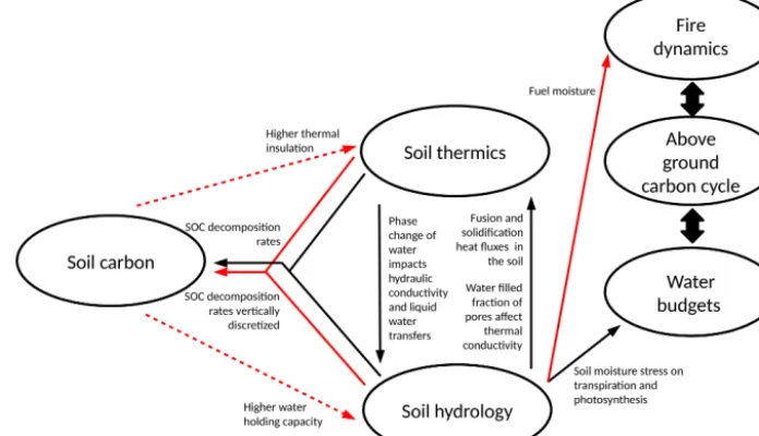
Temperature, water and carbon interactions described in ORCHIDEE revision 3976 are summarized in Fig. 1 by the black arrows. Air temperature and humidity impact phenol-ogy, photosynthesis, autotrophic respiration and the water and heat fluxes comprising the surface energy budget. Soil moisture in the root zone modulates photosynthesis and tran-spiration, which depends on wilting point and field capacity. In ORCHIDEE revision 3976, while soil carbon decompo-sition is impacted by soil water and temperature, soil car-bon stocks themselves exert no feedback on the soil physical state.
The key model developments presented here in ORCHIDEE-MICT (v8.4.1) thus include the feedback effects of soil organic carbon (SOC) concentration on both soil thermic and soil water dynamics (Fig. 1, red arrows). Because these SOC-affected soil physics alter the above- and below-ground components of the carbon cycle, as well as plant transpiration via hydraulic stress, we can expect com-plex indirect effects on the energy, water and carbon budgets (Fig. 1). Note that in the simulations here, soil thermal and hydrological modules read a prescribed observational SOC map (NCSCD in permafrost regions and HWSD in non-permafrost regions) instead of the prognostically simulated SOC, to exclude the impact of bias in the carbon cycle module, for the purpose of model evaluation for the present day in this study. Note that several other updates were
implemented in ORCHIDEE-TRUNK (revision 3976) and passed to ORCHIDEE-MICT (v8.4.1), including a revised background albedo based on satellite observations, and up-dates of the photosynthesis scheme. These will be described in an upcoming paper for ORCHIDEE-TRUNK (version close to revision 3976) that will be used for the CMIP6 exercise. In the following, we describe the parameterizations that define ORCHIDEE-MICT (v8.4.1).
3 High-latitude processes in the initial ORCHIDEE version
3.1 Soil freezing and snow processes
The soil freezing scheme developed by Gouttevin et al. (2012a) describes phase changes of soil water, simulating the latent heat exchanges involved in the freezing and melting of soil water, and subsequent changes in thermal and hydrologi-cal ground properties. Soil heat conductivity and heat capac-ity are dependent on soil ice content. The hydraulic conduc-tivity of the soil is parameterized according to its liquid wa-ter content and decreases with the frozen soil fraction. Heat transfer through the soil column is represented by a one-dimensional heat conduction equation, with latent heat act-ing as a source or sink term (Gouttevin et al., 2012a), in the following function:
c∂T ∂t =
∂ ∂z
λ∂T
∂z
+ρiceL
∂θice
∂t , (1)
where c is volumetric soil heat capacity (J K−1m−3); T is soil temperature (K); λ is soil thermal conductivity (J m−1s−1K−1);ρ
iceis ice density (kg m−3);Lis latent heat
of fusion (J kg−1);θice is volumetric ice content (m3m−3);
t is time (s) andzis depth (m). In ORCHIDEE-MICT, this equation is discretized on the 32 vertical layers of the model with a total soil depth of 38 m (Fig. S1 in the Supplement). Note that the soil hydrology has only 11 layers up to 2 m, so the volumetric contents of water and ice below 2 m take the values of the bottom layer (i.e., the 11th layer).
Figure 1.Temperature, water and carbon interactions in the initial version of ORCHIDEE (black), and processes included in ORCHIDEE-MICT in this study (red). Note that in the simulations in this study, the soil thermics and hydrology modules read a prescribed observation-based soil carbon map (see Eq. 9), which is independent of the prognostically simulated SOC by the carbon module; thus, the two red arrows here are dashed lines.
and will be described in the upcoming CMIP6 ORCHIDEE paper as mentioned in Sect. 2.
3.2 Soil hydrology and river routing
ORCHIDEE simulates soil water fluxes and storage through a multi-layer soil hydrology scheme described by de Rosnay et al. (2000, 2002) and Campoy et al. (2013). Soil moisture is redistributed in the column by solving the Richards equa-tion for vertical unsaturated flow under the effect of root up-take. The hydraulic conductivity and diffusivity depend on soil moisture, following the Mualem–van Genuchten model (Mualem, 1976); (Van Genuchten, 1980), and using param-eters defined by Carsel and Parrish (1988). These variables depend on the dominant soil texture in each grid cell, based on the 12 USDA texture classes provided at the 0.08◦ reso-lution from Reynolds et al. (2000). For frozen soils, the de-crease in the hydraulic conductivity (Gouttevin et al., 2012a) reduces infiltration into the soil and drainage, and increases surface runoff. The 2 m soil column is divided into 11 lay-ers, with layer thickness increasing geometrically with depth (Fig. S1). The saturated hydraulic conductivity is modified according to the scheme in d’Orgeval et al. (2008). This decreases exponentially below a top-30 cm depth boundary to account for increased soil compaction, as suggested by Beven and Germann (1982), and increases above that bound-ary towards the soil surface due to the enhanced infiltra-tion capacity afforded by vegetative roots, whose presence increases soil porosity in the root zone (Beven, 1984). The canopy throughfall rate and soil hydraulic conductivity gov-ern the partitioning between surface runoff and soil
infiltra-tion. This partitioning involves a time-splitting procedure in-spired by Green and Ampt (1911), describing the propaga-tion of the wetting front. The second physical factor con-tributing to total runoff is free gravitational drainage at the bottom of the soil.
The runoff routing module (Polcher, 2003; Ngo-Duc et al., 2005; Guimberteau et al., 2012) aggregates surface runoff and drainage produced at a 30 min time step to calculate daily flow between grid cells and discharge to the ocean. Grid cells are subdivided into basins in which water is trans-ferred through a series of linear reservoirs along the drainage network, derived from a 0.5◦resolution dataset (Vörösmarty et al., 2000; Oki et al., 1999). In a given basin, a “slow” reser-voir collects drainage water, while a “fast” reserreser-voir collects surface runoff, each with different linear response timescales. Corresponding outflows are transferred to the stream reser-voir of the downstream basin. The process is fully detailed in Guimberteau et al. (2012).
M. Guimberteau et al.: ORCHIDEE-MICT, a LSM for the high latitudes 125 4 New processes and parameterizations
4.1 Soil carbon discretization
In ORCHIDEE-MICT, the three soil carbon pools (active, slow and passive) share a common 32-layer discretization scheme with that of soil temperature, to a maximum depth of 38 m. Carbon inflows to the soil pools from decomposed litter are partitioned along this depth using an exponential function that corresponds to the prescribed PFT root profile. Decomposition of soil carbon is calculated at each layer as a function of soil temperature, moisture, and texture (Koven et al., 2009; Zhu et al., 2016). Vertical mixing of soil car-bon due to cryoturbation (mixing of soil layers induced by repeated freeze–thaw cycles) and bioturbation are accounted for by adding a diffusion term in the soil carbon equation:
∂Ci(z, t )
∂t =Ii(z, t )−gi(z, t ) Ci(z, t )+D
∂Ci2(z, t )
∂z2 , (2)
where Ci(z, t ) is carbon content of pool i at depth z and
time t (g C m−3); Ii(z, t ) is carbon input (g C m−3d−1); gi(z, t ) is decomposition rate (d−1);D is diffusive mixing
rate, set as 10−3m2yr−1 through the active layer, and de-creases linearly to zero at 3 m in permafrost regions, to rep-resent cryoturbative mixing (Koven et al., 2009), and set as 10−4m2yr−1above 2 m in non-permafrost regions to repre-sent bioturbation (Koven et al., 2013).
4.2 SOM-dependent soil thermal and hydraulic parameters
Soil organic matter (SOM) significantly modifies soil ther-mal and hydraulic properties. SOM lowers therther-mal conduc-tivity and increases heat capacity (e.g., Lawrence and Slater, 2008; Decharme et al., 2016), and increases soil porosity, which in turn increase saturated hydraulic conductivity and available water capacity (e.g., Hudson, 1994; Morris et al., 2015). As a consequence, the presence of SOM modulates heat transfer from the surface through the soil column, typ-ically leading to cooler soil temperature during summer. SOM-effected increases in soil water holding capacity also enhance plant available water and thus primary productiv-ity (Krull et al., 2004) and transpiration. SOM impacts on soil thermics and hydraulics have previously been parameter-ized in the global LSMs CLM (Lawrence and Slater, 2008), JULES (Chadburn et al., 2015b) and ISBA (Decharme et al., 2016). In ORCHIDEE, SOM thermal insulation was previ-ously investigated by Koven et al. (2009), but its parameter-ization was imbedded in a prior model version which em-ployed bucket-type soil hydrology. This, however, is not ap-plicable to ORCHIDEE-MICT, which uses a new vertically discretized hydrology scheme and its coupling with the ther-mal module. In addition, the Koven et al. (2009) study did not include SOM effects on soil hydraulic properties, which
are addressed in ORCHIDEE-MICT and described in detail below.
Thermal conductivity and heat capacity
By default, soil thermal conductivity and heat capacity in ORCHIDEE are calculated in each soil layer as empirical functions of the 12 USDA soil texture classifications (see Ta-ble S1 in the Supplement) and soil water and ice contents, following F. Wang et al. (2016):
λi=Keiλi,sat+(1−Kei)λi,dry, (3)
with
λi,sat=λ( 1−θi,sat)
i,solid λ
θi,satθi,liqθi,liq+θi,ice
liq λ
θi,satθi,liqθi,ice+θi,ice
ice , (4)
ci =ci,dry+θi,liqcliq+θi,icecice, (5)
where λi,sat and λi,dry are saturated and dry thermal
con-ductivities for layeri;λliq andλice are thermal
conductivi-ties of liquid water and ice, equaling 0.57 and 2.2, respec-tively (W m−1K−1); λi,solid is thermal conductivity of soil
solids (see Table S1);cliqandciceare heat capacities of
liq-uid water and ice, equaling 4.18 106 and 2.11 106, respec-tively (J K−1m−3);cdry is dry soil heat capacity depending
on soil texture;θi,sat is volumetric moisture content at
sat-uration (porosity), and it varies with soil textures;θi,liq and
θi,iceare prognostic volumetric liquid water and ice contents
(m3m−3) that are computed by the soil hydrology model;Kei
is the Kersten number given by the following. For unfrozen soils:
Kei= ( log
10(Sr)+1 0.7 log10(Sr)+1
0
if (
Sr>0.1 0.05< Sr≤0.1
Sr≤0.05
(6)
with Sr=
θi θi,sat
. (7)
For frozen soils:
Kei=Sr, (8)
whereSr is the degree of saturation.
To account for the impacts of organic carbon on soil ther-mal properties in ORCHIDEE-MICT, we follow Lawrence and Slater (2008) in assuming that soil physical properties are weighted averages of mineral soil (as the default values in standard ORCHIDEE) and pure organic soil, with the or-ganic soil fractionfi,soccalculated as
fi,soc=min
1, ρi,soc ρsoc, max
, (9)
where ρi,soc is the carbon content for layer i (kg C m−3),
from NCSCD (Hugelius et al., 2013) in permafrost regions and from HWSD (FAO, 2012) in non-permafrost regions, af-ter linear vertical inaf-terpolation from their original soil hori-zons to fit ORCHIDEE-MICT vertical layers;ρsoc, maxequals
130 kg C m−3, a typical soil carbon density of peat (Lawrence and Slater, 2008). Therefore, the parameters in Eqs. (3)–(7) are calculated as
Pi=(1−fi,soc) Pmineral+fi,socPsoc, (10)
wherePi represents different propertiesλi,dry,λi,solid,ci,dry,
andθi,sat. The values ofPmineralfor each soil texture andPsoc
are listed in Table S1. Note that here we followed Lawrence and Slater (2008) to use linear weighting organic and min-eral soil properties, while in some other models like JULES (Chadburn et al., 2015a) and ISBA (Decharme et al., 2016), soil thermal conductivities are calculated as geometric aver-ages of organic and mineral soils, consistent with the treat-ment for soil water and ice (Eq. 4). The geometric averaging method increases the effect of the organic fraction compared to arithmetic averages, and would be tested in ORCHIDEE-MICT in future developments.
Available water capacity
Plant available water capacity, defined as the difference in the amount of water held by each soil layer between field capac-ity (θfc) and permanent wilting point (θwp), determines the
capacity of the soil to store and supply water for plants, and is therefore an important aspect of soil fertility (Hudson, 1994). For mineral soils in ORCHIDEE, θfc and θwp are derived
from measurements of the soil matric potential at field capac-ity and wilting point, based on the soil water retention curve described by the van Genuchten equation (Van Genuchten, 1980):
θ= (θsat−θr)
1+(α (−9))n
1−1
n
+θr, (11)
whereψis soil matric potential (kPa), andψ= −33 kPa (or
−10 kPa for the three sandy soils; see Table S2) corresponds to field capacity θfc, whileψ= −1500 kPa corresponds to
wilting pointθwpfor all textures;θr is the residual volumetric
water content (m3m−3);αandnare empirical fitting coef-ficients, with their values for different soil textures listed in Table S2.
SOC has been shown to significantly increase water re-tention (Rawls et al., 2003). To parameterize this SOM ef-fect, we assume that θr and the coefficients in Eq. (11) do
not change with carbon content, while porosityθsatincreases
with organic carbon (Eq. 10). Therefore, bothθfcandθwp
in-crease under higher carbon contents, butθfcincreases faster,
resulting in a higher available water capacity (Fig. S2), con-sistent with the patterns observed in Hudson (1994).
4.3 Reformulation of soil hydric stress above the permafrost table
It is known that reduced soil moisture availability decreases the rate of photosynthesis, but the parameterization of this photosynthetic stress differs amongst models (Medlyn et al., 2015). ORCHIDEE-MICT lacks a fully mechanistic plant hydraulic structure that calculates plant internal water move-ment via constraints from water potential (ψ) and conduc-tance of roots, stems and leaves. Instead, a stress factor, which ranges from 0 to 1, is calculated based on the rela-tive moisture content at each soil layer. This factor is applied to stomatal conductance and mesophyll conductance, as well as the maximum RuBisCO activity rate (Vcmax) and maxi-mum electron transport rate (Jmax), in order to account for experimentally observed effects of drought on stomatal and non-stomatal photosynthetic limitation (Zhou et al., 2014). The stress factor (γ) of water limitation is calculated as γi=
θi−θwp
θwp+ρ(θfc−θwp)
, (12)
γ=
11
X
i=1
γiwi, (13)
whereγi is relative moisture content at each soil layer i,
bounded between 0 and 1;ρ represents the fraction above which photosynthesis rate is not limited by soil moisture, and is set at 0.8;wiis the weighting factor for each layer.
In the initial version of ORCHIDEE, the profile ofwi was
assumed to be constant over time, although it differed be-tween tree and grass PFTs, with the highest value at 1.5 m depth for trees and 0.37 m depth for grasses. We considered this description inappropriate for the high latitudes, and in particular for permafrost regions, where trees develop shal-low and lateral roots above the permanently frozen layer (Ka-jimoto et al., 2003). Thus, in ORCHIDEE-MICT,wiis
mod-ified to be a dynamic profile which optimizes plant water use, in a manner inspired by the representation given in Beer et al. (2007):
wi= γi
P11
i=1γi
, (14)
where if layeriis below the modeled active layer thickness, wi is set to zero, and the remainingware re-normalized to
one. 4.4 Fires
M. Guimberteau et al.: ORCHIDEE-MICT, a LSM for the high latitudes 127 and the exclusion of cropland fires to ensure that simulated
mean annual burned area for 1997–2013 was equal to that of the GFED4s dataset. Note that this method only calibrated for mean annual regional burned area, and that simulated lat-itudinal distributions and grid cell spatial patterns of burned area and fire carbon emissions, and their interannual and sea-sonal variabilities, could still be compared with observation-based data. Deforestation and peatland fires are not explic-itly simulated, but as both fire types rely on suitable weather conditions to occur, which could be partly captured by SPIT-FIRE (Yue et al., 2015), model simulations are expected to partially include these fire types.
5 Simulation protocol, forcing and evaluation datasets
5.1 Simulation protocol and forcings 5.1.1 Simulation setup
Two separate runs using different climate forcing input data – CRUNCEP v7 (hereafter CRUNCEP) and GSWP3 – were performed with ORCHIDEE-MICT for the terrestrial North-ern Hemisphere (>30◦N) at 1◦spatial resolution. Both sets of runs encompass the 20th century and the beginning of the 21st century, and were preceded by separate spin-ups for each climate dataset, forced by fixed pre-industrial condi-tions of atmospheric CO2 (286 ppm) and vegetation maps.
The dynamic vegetation model is de-activated throughout both runs. In order to accumulate soil organic carbon in the model, which requires substantial computing time be-fore reaching near-equilibrium in the presence of the slow mixing processes described in Sect. 4.1, the spin-up proce-dure comprised three steps. (1) The full ORCHIDEE-MICT model was forced by looped climate fields over the period 1960–1990 for 100 years to reach equilibria for soil tempera-ture, soil moistempera-ture, vegetation productivity, soil carbon inputs from dead plants, etc. We used the 1960–1990 loop, instead of pre-industrial climate, to approximate the higher Holocene temperatures relative to the “pre-industrial” period that have been reconstructed in Marcott et al. (2013). (2) A soil car-bon sub-model was run for 20 000 years, forced by the out-puts from the preceding step. (3) The full ORCHIDEE-MICT model was run for 100 years, forced by looped 1901–1920 climate data, to approach to the pre-industrial equilibrium for physical variables, carbon fluxes, and fast carbon pools. A fi-nal transient simulation from 1861 to 2007 (using the 1901– 1920 climate loop for the period 1861–1900 due to the lack of climate forcing before the 20th century) was then run from the last year of spin-up stage 3, forced by historical climate forcing and land cover maps, and rising CO2concentrations,
as detailed below.
5.1.2 Atmospheric forcing datasets
The use of two different forcing datasets represents a first step in documenting atmospheric-forcing-based uncertainty in model output. Runoff has been shown for instance to be particularly affected by differences in precipitation from dif-ferent datasets (Fekete et al., 2004; Biancamaria et al., 2009), and by the methods to partition total precipitation volumes between rainfall and snowfall during the cold season (Had-deland et al., 2011). The bias of meteorological drivers also impacts the carbon budget (Zhao et al., 2012). A description of the two datasets used follows.
GSWP3 v0
This 3-hourly 0.5◦global forcing product (1901–2007) was developed for the third phase of GSWP3 (http://hydro.iis. u-tokyo.ac.jp/GSWP3/). It is based on the 20th Century Re-analysis (20CR) version 2 performed with the NCEP land– atmosphere model (Compo et al., 2011). 20CR was dynami-cally downscaled to T248 (0.5◦) resolution using the Global Spectral Model (GSM) by data assimilation using the spec-tral nudging technique (Yoshimura and Kanamitsu, 2008). Bias corrections for precipitation, temperature and longwave and shortwave downward radiations were made using the GPCC v6 (Global Precipitation Climatology Centre), CRU TS v3.21 (Climate Research Unit), and SRB (Surface Radi-ation Budget) datasets, respectively. PrecipitRadi-ation was parti-tioned into rainfall and snowfall referring to the ratio of the downscaled 20CR, and wind-induced undercatch correction (Motoya et al., 2002) was applied separately. We upscaled the GSWP3 forcing for 1◦spatial resolution.
CRUNCEP v7
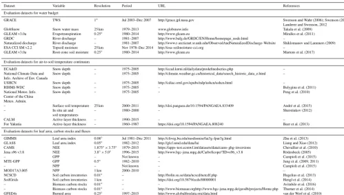
Table 1.List of the datasets used for the ORCHIDEE-MICT evaluation, with their references, the original spatial resolution, and period of availability.
Dataset Variable Resolution Period URL References
Evaluation datasets for water budget
GRACE TWS 1◦ Jul 2003–Dec 2007 http://grace.jpl.nasa.gov Swenson and Wahr (2006); Swenson (2012)
Landerer and Swenson, 2012 GlobSnow Snow water mass 25 km 1979–2013 www.globsnow.info Takala et al. (2009) GLEAM v3.0a Evapotranspiration 0.25◦ 1980–2014 http://www.gleam.eu Miralles et al. (2011)
GRDC River discharge – 1981–2007 http://www.bafg.de/GRDC/EN/Home/homepage_node.html –
Naturalized discharge River discharge – 1981–2007 http://www.r-arcticnet.sr.unh.edu/ObservedAndNaturalizedDischarge-Website Shiklomanov and Lammers (2009) ESA CCI SM v2.2 Topsoil moisture 25 km Nov 1978–Dec 2014 http://esa-soilmoisture-cci.org –
GLEAM v3.0a Root-zone soil moisture 0.25◦ 1980–2014 http://www.gleam.eu Martens et al. (2017)
Evaluation datasets for air-to-soil temperature continuum
ECA&D Snow depth – 1975–2005 http://ecad.knmi.nl/dailydata/predefinedseries.php – National Climate Data and Snow depth – 1975–2005 http://climate.weather.gc.ca/historical_data/search_historic_data_e.html – Info. Archive of Env. Canada
USHCN Snow depth – 1975–2005 http://cdiac.ornl.gov/epubs/ndp/ushcn/ushcn.html –
RIHMI-WDC Snow depth – 1975–2005 – Bulygina et al. (2011)
National Meteo. Info. Snow depth – 1975–2005 – Peng et al. (2010)
Center of the China Meteo. Admin.
– Surface soil temperature 25 km 2000–2011 http://doi.pangaea.de/10.1594/PANGAEA.833409 André et al. (2015)
– In situ air and – 1980–2000 – Sherstiukov (2012)
soil temperatures
CALM Active-layer thickness – 1990–2015 – –
For Yakutia Active-layer thickness – 1960–1987 https://doi.org/10.1594/PANGAEA.808240 Beer et al. (2013)
Evaluation datasets for leaf area, carbon stocks and fluxes
GIMMS Leaf area index 0.08◦ Jul 1981–Dec 2011 http://cliveg.bu.edu/modismisr/lai3g-fpar3g.html Zhu et al. (2013)
GLASS Leaf area index 0.05◦ 1982–2012 http://glcf.umd.edu/data/lai Liang and Xiao (2012)
CAMS NEE 1.875◦×3.75◦ 1979–2015 https://apps-test.ecmwf.int/datasets/data/cams-ghg-inversions Chevallier et al. (2010)
Jena s96 v3.8 NEE 3.8◦×5.0◦ 1996–2015 http://www.bgc-jena.mpg.de/CarboScope/?ID=s96_v3.8 Rödenbeck (2005)
– GPP – Not known – Campioli et al. (2015)
MTE-GPP GPP 0.5◦ 1982–2010 – Jung et al. (2009, 2011)
– NPP – Not known – Campioli et al. (2015)
MOD17A3.005 NPP 1 km 2000–2010 – –
NCSCD Soil carbon inventories 0.01◦ – http://bolin.su.se/data/ncscd/netcdf.php Hugelius et al. (2013)
SoilGrids Soil carbon inventories 1 km – https://doi.org/10.5879/ecds/00000001 Hengl et al. (2014)
– Biomass carbon stocks 0.01◦ – – Avitabile et al. (2016)
– Biomass carbon stocks 0.01◦ – http://www.biomasar.orghttp://www.bgc-jena.mpg.de/geodb/projects/Home.php Thurner et al. (2014)
GFED4s Burned area 0.25◦ 1997–2015 http://www.globalfiredata.org/data.html van der Werf et al. (2010)
and fire emissions
5.1.3 Vegetation and soil texture map
The ESA CCI Land Cover map (Bontemps et al., 2013) was used to produce the PFT map for ORCHIDEE. The ESA CCI land cover product is given by three maps at a 300 m spa-tial resolution, corresponding to the years 2010, 2005 and 2000. These maps were derived from the interpretation of MERIS full and reduced resolutions and SPOT-Vegetation time series. Land cover was classified according to the 22 classes used in the UN-LCCS (land cover classification sys-tem) scheme, which was translated into PFT fractions used in ORCHIDEE, following the cross-walking method presented by Poulter et al. (2011, 2015). Historical land use maps from the Harmonized Global Land Use dataset (Chini et al., 2014) were incorporated to reconstruct PFT fractions since 1860, following Peng et al. (2017), which will be detailed in the upcoming ORCHIDEE-TRUNK paper for CMIP6.
For soil texture, we use the 12 USDA texture classes pro-vided at a global 0.08◦resolution from Reynolds et al. (2000) and upscaled these to the resolution of the atmospheric dataset (1◦×1◦). Only the dominant texture type for a grid cell is used at the 1◦resolution for defining soil hydraulic pa-rameters (Carsel and Parrish, 1988) in ORCHIDEE-MICT.
5.2 Evaluation datasets
The selected datasets used to evaluate ORCHIDEE-MICT are summarized in Table 1 and described in the Appendix. For the water budget evaluation, we selected six Arctic river basins (Fig. 2b) which are important contributors to total Arctic Ocean river inflow: the four largest Eurasian Arctic basins (Ob, Yenisei, Lena and Kolyma), the Mackenzie Basin in northwestern Canada and the Yukon Basin in Alaska. The four Eurasian basins (with the smaller Pechora and Sever-naya Dvina basins) drain about two-thirds of the Eurasian Arctic landmass (Peterson et al., 2002), while the Macken-zie is the largest North American river, bringing freshwater to the Arctic Ocean (Woo and Thorne, 2003). We also eval-uated the Volga Basin (Fig. 2b), which is subject to snowfall events during the year but is not underlain by permafrost, in order to compare results with the high-permafrost Arctic basins (Fig. 2a and Table S4).
M. Guimberteau et al.: ORCHIDEE-MICT, a LSM for the high latitudes 129
Figure 2. (a)The three high-latitude sub-regions used in this study, including boreal North America (BONA), boreal Europe (BOEU) and boreal Asia (BOAS), following McGuire et al. (2016). Blue and red lines indicate the extent of continuous permafrost and all permafrost categories, respectively, according to the IPA permafrost map (Brown et al., 2002).(b)The seven high-latitude basins selected for this study with the gauge stations (red circles on the map, more information in Table S4).
temperature gradients between the near-surface and deeper soils.
6.1 Snow insulation controls on the temperature gradient between air and topsoil
6.1.1 Snow depth
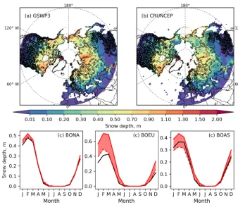
ORCHIDEE-MICT correctly captures the spatial distribu-tion of maximum monthly average snow depth (Fig. 3a, b), and the seasonal decrease in snow depth from March to June (Fig. 3c), but modeled snow depth strongly depends on the atmospheric forcing used. GSWP3 climate forcing tends to produce a larger maximum snow depth than CRUNCEP, greater than those observed in all northern regions, especially over boreal Europe (BOEU) (Fig. 3c). This shows that uncer-tainty from climate forcing data is as large as the model bias compared with observations, making it difficult to attribute a model bias to a particular component of the snow model. However, the rate of sublimation in winter (Pomeroy et al., 1998) and the prescribed albedo value of fresh snow have been shown to be critical in determining the peak value and phase of both snow depth and SWE (T. Wang et al., 2015). 6.1.2 Snow conductivity and snow density
Mean snow density and mean snow thermal conductiv-ity are computed at the month of maximum snow depth over the 1981–2007 period as weighted averages over the three snow layers. Gouttevin et al. (2012b) report density values of 200 kg m−3 for taïga and 330 kg m−3 for tun-dra and conductivity values of 70 mW m−1K−1 for taïga and 250 mW m−1K−1 for tundra, from Sturm and John-son (1992) and Domine et al. (2010). These higher values
over tundra were attributed to snow compaction by wind. This process is not modeled in ORCHIDEE-MICT and we thus simulate similarly high values of conductivity for both biomes (Fig. S3): approximating tundra with C3 grass PFT between 55 and 85◦N, and taïga with the boreal forests PFTs between 45 and 70◦N and considering only grid cells with a fraction of the dominant biome above 0.6. The model yields a mean snow conductivity of 266±203 (GSWP3) and 219±197 (CRUNCEP) mW m−1K−1for tundra com-pared to 221±113 (GSWP3) and 182±100 (CRUNCEP) mW m−1K−1 for taïga and a mean density of 269±102 (GSWP3) and 239±103 (CRUNCEP) kg m−3for tundra and of 233±67 (GSWP3) and 207±63 (CRUNCEP) kg m−3 for taïga. Note that a recent study (Domine et al., 2016) sug-gests for tundra a complex structure with depth-hoar devel-oping at the base of snowpack during the course of the snow season, causing conductivities as low as 20 mW m−1K−1in late winter, whereas snow-compacted upper layers have con-ductivities of 200 to 300 mW m−1K−1, more comparable to ORCHIDEE-MICT.
6.2 Summer land surface temperature
Figure 3.Maximum monthly snow depth (m) simulated (background maps) with(a)GSWP3 and(b)CRUNCEP forcings compared to observations (color filled circles), averaged over the period 1975–2005.(c)Monthly mean seasonal snow depth (m) from observation and the two simulations, averaged over the observation sites in the three high-latitude sub-regions (shown in Fig. 2a).
6.3 Soil temperature
The simulated spatial patterns of mean annual topsoil (0.2 m) temperature generally reproduce the observed gradient along a southwest–northeast transect in Siberia (Fig. 5a, b). How-ever, the CRUNCEP-forced simulation results are colder than those from the GSWP3 ones as well as relative to observa-tions in the permafrost region (Fig. 5a, b), mainly driven by a strong cold bias in CRUNCEP-based winter soil tempera-tures (Fig. 5c, d).
During winter, the snowpack acts as an insulating layer above the soil surface, reducing soil heat loss. Snow thus causes a large positive temperature gradient (1T), which is controlled by both snow depth and snow thermal proper-ties, such as thermal conductivity, density and albedo. Gen-erally, the model underestimates snow insulation in the early (November to January) and late (February to April) cold sea-sons for the same snow depth, as compared to observations (Fig. 6). This indicates that relatively congruent wintertime soil temperatures in the GSWP3-forced simulation in per-mafrost regions (Fig. 5c) may be due to a bias compensation from overestimated snow depth (Fig. 3) and underestimated snow thermal insulation.
A prominent component of the1T–snow depth relation-ship observed at Russian stations (black in Fig. 6) is the
sig-nificantly lower insulation during the late cold season, prob-ably due to snow compaction and densification leading to higher snow conductivity (Decharme et al., 2016). This dif-ferential sensitivity of1T to snow depth between the two pe-riods is effectively captured by ORCHIDEE-MICT, despite small modeled negative1T values (i.e., topsoil colder than air) compared to observations at the termination of the snow season, when snow depth is diminished (<20 cm).
M. Guimberteau et al.: ORCHIDEE-MICT, a LSM for the high latitudes 131
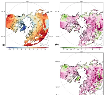
Figure 4. (a)Observed mean summer (JJA) land surface temperature (◦C) and bias in the(b)GSWP3 and(c)CRUNCEP-forced simulations, averaged over the period 1996–2007.
would partly offset the warm bias in CRUNCEP land surface temperatures during summer (Fig. 4c).
6.4 Active layer thickness and permafrost area
Figure 7a, b show the simulated spatial pattern of ALT, as calculated from modeled soil temperatures using a linear interpolation between soil layers to locate the first depth that remains frozen (below 0◦C) year-round. Compared with CALM observations, in which most of the sites have ALT<1 m, the GSWP3-forced model generally overesti-mates ALT by more than 1 m (also see Fig. S5, which compares modeled ALT of Yakutia, eastern Siberia with the map of Beer et al., 2013), whereas CRUNCEP-forced output shows relatively better agreement with the observa-tions. Apart from the uncertainty induced by climate forc-ing, the model–data mismatch may also arise from scale dif-ferences for the organic carbon content that is used to cal-culate soil physical properties for each grid cell. As men-tioned in Sect. 4.2, the empirical SOC map from NCSCD (Hugelius et al., 2013) is prescribed for permafrost regions in the soil thermal and hydrological modules, which is up-scaled by the model to the target spatial resolution (1◦ by 1◦ in this study). These SOC values thus do not represent
the site-level soil conditions, aside from the uncertainty of the NCSCD database itself. To further investigate this im-pact, we conducted additional simulations for the sites that provide explicit organic layer thicknesses (in total, 69 sites), forced by CRUNCEP. In these runs, we assumed pure or-ganic soil, i.e.,fi,SOC in Eq. (9) equaling one, for the soil
layers above the site-specific organic layer thickness, but kept the SOC concentration unchanged below this thickness, i.e., from NCSCD. Note that the moss layer, vegetation mat, and/or organic root zone as described in some sites were all summed to derive a total organic layer thickness. The other configurations including climate forcing and soil tex-ture were the same as the regional simulation. The result is displayed in Fig. S6, showing significantly shallower ALTs simulated by these site runs which better match the observa-tions (Fig. S6a), with different magnitudes of ALT reducobserva-tions among the sites (Fig. S6b).
Figure 5.Mean annual soil temperature at 0.2 m depth (◦C) in the(a)GSWP3 and(b)CRUNCEP-forced simulations (background maps), compared to the site observations (color filled circles), averaged over the period 1981–2000. Monthly mean seasonal soil temperatures at different depths (◦C) in the(c)GSWP3 and(d)CRUNCEP-forced simulations, compared with the observation, averaged over the 51 sites in continuous permafrost region (according to the IPA map) and over the period 1981–2000. The spatial patterns of maximum monthly soil temperature are also shown in Fig. S4.
Figure 6.Relationship between1T (soil temperature at 20 cm depth minus air temperature) and snow depth (cm) over the period 1981–2000, for site-level observations (black), and for model results (red) (9612 site-month values in total), forced by(a)GSWP3 and(b)CRUNCEP. Circles and squares are medians of 5 cm snow depth bins, representing the early (November–January) and late (February–April) snow season, respectively. Upper and lower bars indicate the 25th and 75th percentiles of each bin. The size of circles/squares indicates the frequency of occurrence in each bin.
with differing soil vertical discretizations may include uncer-tainties brought by the arbitrarily chosen definition, whereas evaluation and comparison directly for soil temperatures and ALT should be more robust. A qualitative comparison against the empirical IPA (International Permafrost Association) per-mafrost map (Brown et al., 2002) shows better agreement for CRUNCEP compared to GSWP3-forced output, since CRUNCEP-forced simulation generally matches the distri-bution of continuous permafrost using the former definition, while GSWP3-forced simulation seems to underestimate
per-mafrost extent (Fig. 7c, d). This is consistent with the deeper simulated ALT under GSWP3 climate forcing.
M. Guimberteau et al.: ORCHIDEE-MICT, a LSM for the high latitudes 133
Figure 7.Active layer thickness (ALT in m) from the(a)GSWP3 and(b)CRUNCEP-forced simulations (background maps), compared to the observed ALT from the CALM network (color filled circles), averaged over the period 1990–2007. Permafrost extent from the(c)GSWP3 and(d)CRUNCEP-forced simulations according to two different definitions (yellow and red lines) on top of the IPA permafrost map (Brown et al., 2002).
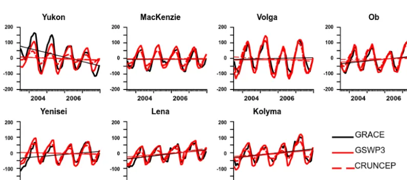
Figure 8.Interannual monthly variation and trend (line) of TWS (mm) simulated with the two forcings compared to GRACE data over the seven basins (see Fig. 2b), for the period July 2003–December 2007.
with attendant impacts on Arctic Ocean discharge and sub-basin-scale water budgets. Here, only sub-basin-scale averages are discussed.
7.1 Total terrestrial water storage change
A realistic phase and amplitude of TWS are simulated with both forcing datasets, although peak-to-peak amplitude is
with both forcings, at the seasonal scale and for the 5-year trends, except in the Yukon Basin, where observed TWS de-creases are not reproduced in our simulations, with no pre-cipitation decrease in the GSWP3-forced model. The Yukon TWS decline is likely due to glacier melt in the northwestern Cordillera (S. Wang et al., 2015). As glaciers are not rep-resented in ORCHIDEE-MICT, the model does not capture these TWS trends. Note that groundwater storage changes re-lated to the development of closed and open taliks (Muskett and Romanovsky, 2009) which contribute to existing TWS trends – increasing storage in the Lena and Yenisei, decreas-ing it in the Mackenzie Basin, and no change in the Ob – are not modeled either in ORCHIDEE-MICT. Despite this, the model reproduces observed trends in these basins.
7.2 Snow-related processes controlling land water storage in the cold season
The modeled seasonal cycle of the SWE and the length of the snowmelt period are in agreement with observations (Fig. 9), suggesting a good parameterization of the snowmelt and sub-limation processes. However, results differ strongly accord-ing to forcaccord-ing inputs. In basins with a large permafrost frac-tion (Yukon, Lena and Kolyma) and, to a lesser extent, in the Mackenzie, Ob and Yenisei basins, SWE is underesti-mated throughout the year compared to GlobSnow data when ORCHIDEE-MICT is forced by CRUNCEP, and it is signif-icantly larger in the GSWP3-forced simulation (in the Volga Basin, the SWE is overestimated in the two simulations). This is due to the low basin-specific snowfall rate in CRUN-CEP forcing compared to GSWP3 (Fig. S12), which is prob-ably the result of the criterion used to partition rainfall and snowfall in CRUNCEP, and strongly affects the simulation of snow depth and SWE (Loth et al., 1993; Wen et al., 2013). By contrast, the GSWP3-forced model captures the early winter SWE accumulation in these basins. In spring, the SWE is sys-tematically overestimated except over the Lena, whose sea-sonal cycle is well reproduced by ORCHIDEE-MICT. This corresponds to an excessive persistence of the snow cover, which may be explained by the absence of hysteresis in the snow depletion curve relating the snow cover extent and the SWE (e.g., Magand et al., 2014). In the Yenisei and Macken-zie basins, the SWE in winter is closer to observations with the GSWP3 forcing, with the exception of springtime val-ues, which are better under CRUNCEP forcing. In basins where the permafrost area is near-zero (Ob and Volga), the SWE from CRUNCEP-forced simulation is closer to Glob-snow than those from GSWP3, in which SWE is overesti-mated in winter and spring. This is related to the large differ-ence in snowfall over these basins between the two forcings (Fig. S12).
7.3 Soil moisture In the topsoil
Seasonal evolution of topsoil moisture (first 2 cm) is com-pared to the ESA-CCI-SM product over the seven basins (Fig. 10a). Liquid soil moisture values from the model are used for the comparison because the ESA-CCI-SM prod-uct measures only the topsoil moisture when temperature is above 0◦C. Because of scaling issues (the satellite product is rescaled to the 10 cm top layer of the NOAH model, as al-ready noted, but is more representative of a thinner soil layer of about 2 cm), the comparison was performed on relative liquid soil moisture values after normalization with their re-spective SD. The observed seasonal moisture variations are captured well by ORCHIDEE-MICT with both forcings over the seven basins (Fig. 10a). The maximum values occur in summer, in contrast to lower latitudes, because of the thaw-ing processes occurrthaw-ing in summer. The local minimum sim-ulated in summer in the Volga and Ob basins is underesti-mated, suggesting a too slow infiltration front of the water in the topsoil layers of the model. Thus, less water in the root zone is available for transpiration, which is found to be underestimated when compared to GLEAM (see Fig. 11b). Compared to observations, a more rapid increase (decrease) in the modeled topsoil moisture in spring during snowmelt (in fall) is found in the Yukon and Mackenzie basins, related to a more rapid thawing (freezing) of the topsoil.
In the root zone
M. Guimberteau et al.: ORCHIDEE-MICT, a LSM for the high latitudes 135
Figure 9.Monthly mean seasonal SWE (mm) simulated with the two forcings compared to GlobSnow over the seven basins (see Fig. 2b), averaged over the period 1981–2007.
Figure 10.Monthly mean seasonal relative(a)topsoil (–) and(b)root soil moisture (–), both normalized by their multi-year SD, simulated with the GSWP3 and CRUNCEP forcings over the seven basins (see Fig. 2b), averaged over the period 1981–2007. The results are compared with(a)satellite-derived observations from ESA CCI and(b)the GLEAM data-driven model assimilated against satellite data.
7.4 Evapotranspiration and component fluxes
The amplitude of the ET seasonal cycle is generally well cap-tured by the model in most basins, when compared to the GLEAM product, despite a systematic underestimation by
Figure 11. (a)Monthly mean seasonal evapotranspiration (mm d−1) simulated with the two forcings compared to the GLEAM data-driven model over the seven basins (see Fig. 2b), averaged over the period 1981–2007.(b)Seasonal bias of ET components (mm d−1) averaged over the same period, with the GSWP3 (solid line) and CRUNCEP (dashed line) forcings.
underestimated in spring and early summer for both forcings, except in the Volga Basin. This is consistent with modeled LAI increasing too late in spring (see Fig. 13), which could be due, at least partially, to an excessive persistence of the snow cover in spring. In fall, the timing of the decrease in ET is reproduced by both forcings. Model biases with re-spect to GLEAM data in the sublimation, soil evaporation and transpiration components of ET are shown in Fig. 11b. In all basins, sublimation bias in simulations forced by GSWP3 is ∼0 in winter, in agreement with GLEAM. By contrast, CRUNCEP-forced simulations slightly overestimate subli-mation in early spring across basins with the exception of the Volga. These results are consistent with SWE underesti-mation (except in the Volga) (Fig. 9) and higher downward shortwave radiation (Fig. S14) that results when CRUNCEP forcing is used. The general underestimation of summer ET by ORCHIDEE-MICT in the Yukon, Mackenzie and Kolyma basins is explained mainly by a too low transpiration despite bare soil evaporation being slightly overestimated (Fig. 11b). When forced by CRUNCEP data, ORCHIDEE-MICT over-estimates interception loss in all basins but the Kolyma and Yukon, which is consistent with CRUNCEP LAI overestima-tion (see Fig. 13).
7.5 River discharge
By comparing the two simulations, it is clear that the mete-orological forcing exerts a significant influence on the sim-ulated river discharge (Fig. 12): GSWP3 leads to systemat-ically higher river discharge than CRUNCEP, which is per-fectly consistent with the SWE biases (Fig. 9). In a ma-jority of basins, GSWP3-forced simulations better capture the seasonal cycle of observed discharge than CRUNCEP-forced ones, especially in the Yukon and eastern Siberian basins, where the discharge is strongly underestimated under CRUNCEP forcing (between 60 % in the Yenisei and 83 % in the Yukon).
reser-M. Guimberteau et al.: ORCHIDEE-MICT, a LSM for the high latitudes 137
Figure 12.Monthly mean seasonal river discharge (m3s−1) simulated with the two forcings compared to the observed non-naturalized (GRDC) and Siberian naturalized river discharge dataset at the gauge stations of the seven basins (see Fig. 2b), averaged over the period 1981–2007.
Figure 13.Monthly mean seasonal LAI (–) simulated with the two forcings compared to GIMMS and GLASS products over the seven basins (see Fig. 2b), averaged over the period 1981–2007.
voirs. No natural lakes are simulated by ORCHIDEE-MICT, which may contribute to the winter discharge underestima-tion, especially for the Mackenzie, which includes massive lakes (Great Slave, Great Bear, and Athabasca).
The nival regime of the studied basins is also characterized by peak flow in late spring, which is broadly captured by the ORCHIDEE-MICT simulations, even if the magnitude of peak flow is strongly biased in some cases, with a strong link to the forcing used and the SWE biases. As an exam-ple, the Volga is the only river where both peak flow and SWE are overestimated with both forcings, and closer to river discharge observations under the CRUNCEP forcing. In this human-altered basin, the absence of the simulation of water withdrawals for irrigation in the model can explain the peak flow overestimation.
An almost systematic weakness of the simulated hydro-graphs is the underestimation of river discharge during
soils, which appear to be too drastic in their prevention of snowmelt infiltration under conditions of frozen topsoils. Al-ternative parameterizations of these dynamics are underway. For example, infiltration of meltwater into frozen soil could be permitted when accounting for sub-grid-scale variability of topsoil freezing and drying which would enhance infiltra-tion (Gray et al., 2001). Other perspectives are the improve-ment of the floodplain parameterization in ORCHIDEE-MICT (Lauerwald et al., 2017) and the inclusion of natural lakes and artificial reservoirs.
8 Evaluation of the leaf area index, gross and net CO2 fluxes
8.1 Leaf area index
According to the two evaluation products, the seasonal cy-cle of LAI (Fig. 13) is similar across the basins, with val-ues near zero during winter, and a maximum in summer. There is a consistent phasing of seasonal LAI between the two evaluation datasets; however, maximum LAI in GIMMS is systematically higher than in GLASS. In all the basins, the LAI simulated by ORCHIDEE-MICT has a phase delay of up to 1 month compared to both products. This is due to a delay in the start of the growing season, which may be re-lated to excessive persistence of the snow cover (Fig. 9). The phenological models in ORCHIDEE (detailed in MacBean et al., 2015, Appendix A) do not explicitly take into ac-count this influence, unlike what is done in Van Wijk et al. (2003), who model the link of the start of the tussock tun-dra growing season to the soil thaw at 10 cm depth. How-ever, there is a first indirect link between the snow cover and the vegetation phenology through air temperature, which in-fluences both the start of the growing season, determined in ORCHIDEE using growing degree days (GDD)-based phe-nological models for deciduous species, and the start of the snowmelt season. There is a second indirect link through snowmelt. While there is still a large amount of snow, the soil surface temperature is kept at zero degree Celsius or be-low, and the soil cannot thaw. Only when snowmelt occurs and when the snow fraction is small enough will the soil start thawing, thus increasing soil liquid water content. This im-pacts the start of the growing season for grasses and crops, which use both a GDD and a soil moisture thresholds, and also reduces water stress, thus favoring photosynthesis for all PFTs. Note here that ORCHIDEE-MICT is prone to over-estimating the timing of senescence (MacBean et al., 2015). This is true in particular for conifers, for which the model lacks an explicit senescence inception model. Except in the Yukon and Mackenzie basins, the maximum LAI simulated by ORCHIDEE-MICT lies between the two satellite prod-uct estimates. Winter LAI of∼1.0 are overestimated in the Yukon, Mackenzie, Ob and Yenisei basins; however, obser-vations show values around zero. Given that these basins are
covered by a larger fraction of evergreen forests compared to the others, these simulated values look reasonable. The mis-match with the observations could be explained here by data errors, the assessment of solar reflectance from space in win-ter at the high latitudes being less reliable.
8.2 Gross (GPP) and net (NPP) primary productivity 8.2.1 Spatial distribution and seasonal cycle of GPP GPP at the high latitudes is co-limited by cold temperatures, constraining the duration of the growing season, and by sum-mer water stress (Schulze et al., 1999) in northern Canada and Siberian boreal forests, for which the water balance is usually negative at this time. The simulated spatial pattern of GPP in Eurasia and North America is close to the MTE-GPP dataset (Fig. 14). Values lower than MTE-GPP were simu-lated in eastern Siberia under the GSWP3 forcing, mainly due to water stress (see also the underestimated biomass for eastern Siberia in Fig. 20). The seasonal GPP cycle in Fig. 14b is generally accurate with respect to observations at the scale of large boreal regions; however, peak GPP is strongly overestimated for boreal North America (BONA).
Interestingly, comparing GPP forced by the two climate datasets shows higher values by CRUNCEP than by GSWP3 (Fig. 14), despite a generally lower precipitation in CRUN-CEP (Fig. S13). This could be explained by the higher spe-cific air humidity during summer in CRUNCEP than in GSWP3 (Fig. S16). A low air humidity increases the atmo-spheric vapor pressure deficit (VPD) and the leaf-to-air vapor pressure difference; plants then partially close the stomata to constrain a potentially fast transpiration (Oren et al., 1999; McAdam and Brodribb, 2015), which leads to a reduced photosynthetic rate. The photosynthesis module in OR-CHIDEE largely follows Yin and Struik (2009), in which stomata conductance decreases with an increasing VPD, and thus is able to simulate a lower GPP under dry air conditions. A recent study (Novick et al., 2016) showed that, between the two factors that impact plant water stress, i.e., soil mois-ture supply and atmospheric demand for water (reflected by VPD), the latter limits evapotranspiration to a greater extent than the former in relatively wet forested ecosystems. In spite of its importance, the effect of VPD on vegetation productiv-ity has been far less studied than soil water availabilproductiv-ity (Kon-ings et al., 2017), warranting further investigations in both observations and land surface models.
8.2.2 Spatial distribution of NPP and site-level comparison
M. Guimberteau et al.: ORCHIDEE-MICT, a LSM for the high latitudes 139
Figure 14. (a)Simulated annual GPP (g C m−2day−1) from the two climate forcings, compared to the data-driven MTE-GPP, averaged over the period 2000–2007.(b)Monthly mean seasonal GPP (g C m−2day−1) simulated with the two forcings compared to MTE-GPP over the three high-latitude sub-regions (shown in Fig. 2a), averaged over the same period.
Figure 15.Mean annual NPP (g C m−2yr−1) simulated with(a)GSWP3 and(b)CRUNCEP forcings (background maps) compared to the site observations (color filled circles), averaged over the period 2000–2007.
and Siberia, the model is able to reasonably capture NPP gradients in BONA and BOEU. In temperate forests of western Europe and the eastern US, modeled NPP is too low (see also Fig. 16b for warm sites), possibly due to high water stress in ORCHIDEE-MICT (see below).
Considering only the 52 sites that were selected (as de-scribed in Appendix C3), we computed the distributions of GPP and NPP by 5◦C mean annual temperature bins for the sites, the MTE-GPP and MODIS-NPP products, and for the ORCHIDEE-MICT simulations. We plot the 95th percentiles of these distributions in Fig. 16, which arguably defines an
Figure 16.95th percentiles of mean annual(a)GPP (g C m−2yr−1) and(b)NPP (g C m−2yr−1) distributions per temperature bins of 5◦C for in situ measurements, the gridded MTE-GPP (MODIS-NPP) product sampled at the sites’ locations and the two simulation results, averaged over the period 2000–2007.
Figure 17.Mean annual CUE (%) over the 52 Campioli sites, aver-aged over the period 2000–2007. The first black boxplot is com-puted using the local estimations of the Campioli et al. (2015) database and the second one (global observations) using MODIS-NPP and MTE-GPP. The red boxplots use the values of the two sim-ulations. For each boxplot the median value is the short horizontal bar within the rectangle, whose bottom and top sides illustrate the 25th and 75th percentiles of the distribution, while the vertical seg-ments link those sides to the points representing, respectively, the minimum and maximum values.
local sites, whereas modeled GPP and NPP saturate for tem-peratures above 10◦C, indicating water stress dominant con-trols.
The local measurements and the global observations prod-ucts give similar median CUE values (51 and 49 %, respec-tively) and first and third quartiles, whereas the model gives a narrower distribution range, with higher median values (57 % for GSWP3 and 53 % for CRUNCEP) (Fig. 17). 8.3 Spatial distribution of burned area and fire
emissions
The spatial distribution of burned area is largely reproduced by ORCHIDEE-MICT, with a higher fraction of burned area in central Eurasia, and a decrease in burned area toward higher latitudes (Fig. 18). For the GSWP3 simulation, mod-eled total burned area over the period 1997–2007 (in the unit of Mha yr−1) is smaller than GFED4s for BONA (1.7 vs. 2.2
in GFED4s), and higher for BOEU (8.1 vs. 5.0) and BOAS (16.1 vs. 10.4). Modeled spatial distribution of natural fire emissions has greater discrepancies with respect to evalu-ation data than burned area, bearing in mind that GFED4s data are based on a biosphere model (CASA), not observa-tions. Higher emissions in eastern Eurasia are reproduced by ORCHIDEE-MICT. However, modeled emissions are over-estimated for central Eurasia and underover-estimated in boreal America, with respect to GFED4s. As a result, regional car-bon emissions (in the unit of Tg C yr−1) in ORCHIDEE-MICT are lower than in GFED4s for BONA (20 vs. 48), much higher for BOEU (45 vs. 6), and in good agreement for BOAS (104 vs. 111). One possible reason for the discrepancy in BOEU is the lack of forest management and fire suppres-sion measures in ORCHIDEE-MICT, leading to higher sim-ulated burned area and carbon emissions than in GFED4s. Changing the climate forcing from GSWP3 to CRUNCEP yields a smaller burned area (Fig. 18b and c). Because the re-duction of burned area mainly occurs in grassland, the impact on carbon emission is small.
M. Guimberteau et al.: ORCHIDEE-MICT, a LSM for the high latitudes 141
Figure 18. (a–c)Mean annual fractional burned area (%) from(a)satellite observation in GFED4s and(b)GSWP3 and(c)CRUNCEP-forced simulations.(d–f)Mean annual carbon emissions from natural fires (g C m−2yr−1) from(d)satellite observation in GFED4s and(e)GSWP3 and(f)CRUNCEP-forced simulations, averaged over the period 1997–2007. The burned area fraction simulated from ORCHIDEE-MICT is corrected for the omission of cropland fires in the simulation.
However, for BONA the fire season starts 1 month later in ORCHIDEE-MICT (Fig. S7a). For BOAS and BOEU, there are stronger discrepancies in seasonal carbon emis-sion (Fig. S7e, f). In particular, ORCHIDEE-MICT fails to account for the April peak in carbon emissions. A possible explanation for the missing April emissions in ORCHIDEE-MICT may be the late timing of snowmelt (Fig. 9) and the delayed spring increase in LAI (Fig. 13). This would cause an unavailability of fuel in springtime. Changing the climate forcing from GSWP3 to CRUNCEP has only a very small effect on burned area and carbon emission seasonality. 8.4 Seasonal cycle of NEE
Monthly NEE from inversions, originally provided at the spatial resolution of each transport model, was aggregated at the scale of the three high-latitude sub-regions (Fig. 2a). Spatially averaged NEE is expected to be more consistent between different inversions at a coarser spatial scale, given the sparseness of atmospheric CO2stations and differences
in transport models. Nevertheless, the seasonal cycle of NEE is generally consistently estimated by the two inversions in each sub-region, although Jena CarboScope estimates gen-erally higher seasonal NEE amplitude, and in BOEU NEE from CAMS peaks 1 month earlier than Jena CarboScope (Fig. 19). Simulated seasonal NEE (defined as GPP minus autotrophic and heterotrophic respiration, fire emissions and
emissions from LUC) magnitude and evolution is very sim-ilar in both simulations and, in general, ORCHIDEE-MICT was able to reproduce the timing and magnitude of the tran-sition between winter release and spring NEE uptake, despite a later onset of spring uptake for all three boreal sub-regions, and a smaller peak summer NEE for BOAS.
Since the timing of NEE uptake in spring and release in fall is well constrained in the inversions from the observed periodical drawdown and buildup of CO2at atmospheric
sta-tions, the modeled delayed onset of spring uptake is consis-tent with the∼1-month lag between ORCHIDEE-simulated and satellite-observed LAI in Fig. 13 (and ET in Fig. 11a) in the basins of the three sub-regions. Even though GPP is over-estimated in BONA during spring and summer (Fig. 14b), the resulting NEE gives a slightly weaker uptake.
Figure 19.Monthly mean seasonal net land–atmosphere CO2fluxes (NEE in Pg C month−1) from the GSWP3 and CRUNCEP-forced
simulations compared to atmospheric inversions, over the three high-latitude sub-regions (shown in Fig. 2a), averaged over the period 2000– 2007. The grey shaded areas correspond to the SD of the monthly values for each inversion. Note that a negative sign in NEE corresponds to CO2uptake from the atmosphere, and a positive sign to release into the atmosphere.
mosses and lichens which could have respiration under win-ter low temperatures (Atanasiu, 1971). This suggests that we should either allow decomposition below the freezing point, perhaps to account for heat produced in the soil by microbial decomposition (Zimov et al., 1993; Hollesen et al., 2015), improve the snow insulation, prescribe an organic layer of in-sulating topsoil (e.g., mosses, O-horizons observed in boreal forests; see O’Donnell et al., 2011) into the thermal module, or explicitly represent the moss/lichen plants, including their carbon cycle and physical effects (Porada et al., 2016; Druel et al., 2017).
NEE discrepancies may be related to the different sea-sonal contributions of evergreen and deciduous trees to GPP and LAI (Fig. S9), as well as to the relative sensitivity of heterotrophic respiration, autotrophic respiration and distur-bances to the warming (cooling) at the beginning of the grow-ing season (winter).
9 Evaluation of carbon stocks 9.1 Biomass
Consistent with the LAI and GPP results, the simulation forced by CRUNCEP shows higher forest biomass carbon densities than the GSWP3 simulation (Fig. 20). The two sim-ulations, however, exhibit similar patterns, which reproduce the general spatial pattern of observed biomass, being higher in the western and eastern regions of North America, with a declining gradient across Eurasia from the west to the east. However, in general, the model tends to overestimate car-bon density in regions of observed high carcar-bon density (e.g., northwestern Europe and European Russia, eastern North America, the Korean Peninsula and Japan). The model also misplaced the region of the highest biomass density in north-western Europe and European Russia rather than central Eu-rope as shown by the observation data. Likewise, the model estimates extremely large biomass in eastern North America, especially by CRUNCEP forcing, which almost doubles the observed amount. For the rest of the study region, simulated carbon density is slightly lower than observations, by around
5–25 Mg C ha−1. The two observation datasets show consid-erable similarities.
M. Guimberteau et al.: ORCHIDEE-MICT, a LSM for the high latitudes 143
Figure 20.Total forest biomass carbon density (Mg C ha−1) from the(a)GSWP3 and(b)CRUNCEP-forced simulations compared with satellite-derived observation products from(c)Avitabile et al. (2016) and(d)Thurner et al. (2014), averaged over the period 2000–2007.
Figure 21. Soil organic carbon from the GSWP3 and CRUNCEP-forced simulations compared with the two inventory datasets NC-SCD (Hugelius et al., 2013) and SoilGrids, averaged over the period 2000–2007.(a)Spatial distribution (kg C m−2).(b)Vertical profiles (kg C m−3) averaged over the three high-latitude sub-regions (shown in Fig. 2a). Since NCSCD does not encompass the whole domain, only grid cells with available data in NCSCD are averaged for BONA and BOAS so that the four vertical profiles are comparable, while for BOEU, NCSCD is not shown, as it has few data in this sub-region.
9.2 Soil carbon
SOC stocks simulated by the model fit to some extent the one of the observed inventory data, including that of NCSCD’s permafrost region near-surface SOC density (Fig. 21), but