https://doi.org/10.5194/essd-9-529-2017 © Author(s) 2017. This work is distributed under the Creative Commons Attribution 3.0 License.
A global data set of soil hydraulic properties and
sub-grid variability of soil water retention and
hydraulic conductivity curves
Carsten Montzka1, Michael Herbst1, Lutz Weihermüller1, Anne Verhoef2, and Harry Vereecken1,3 1Forschungszentrum Jülich GmbH, Institute of Bio- and Geosciences: Agrosphere (IBG-3), Jülich, Germany
2University of Reading, Department of Geography and Environmental Science, Reading, UK 3International Soil Modeling Consortium, Jülich, Germany
Correspondence to:Carsten Montzka (c.montzka@fz-juelich.de)
Received: 14 February 2017 – Discussion started: 23 February 2017 Revised: 19 June 2017 – Accepted: 19 June 2017 – Published: 27 July 2017
Abstract. Agroecosystem models, regional and global climate models, and numerical weather prediction mod-els require adequate parameterization of soil hydraulic properties. These properties are fundamental for describ-ing and predictdescrib-ing water and energy exchange processes at the transition zone between solid earth and atmo-sphere, and regulate evapotranspiration, infiltration and runoff generation. Hydraulic parameters describing the soil water retention (WRC) and hydraulic conductivity (HCC) curves are typically derived from soil texture via pedotransfer functions (PTFs). Resampling of those parameters for specific model grids is typically performed by different aggregation approaches such a spatial averaging and the use of dominant textural properties or soil classes. These aggregation approaches introduce uncertainty, bias and parameter inconsistencies throughout spa-tial scales due to nonlinear relationships between hydraulic parameters and soil texture. Therefore, we present a method to scale hydraulic parameters to individual model grids and provide a global data set that overcomes the mentioned problems. The approach is based on Miller–Miller scaling in the relaxed form by Warrick, that fits the parameters of the WRC through all sub-grid WRCs to provide an effective parameterization for the grid cell at model resolution; at the same time it preserves the information of sub-grid variability of the water retention curve by deriving local scaling parameters. Based on the Mualem–van Genuchten approach we also derive the unsaturated hydraulic conductivity from the water retention functions, thereby assuming that the local parameters are also valid for this function. In addition, via the Warrick scaling parameterλ, information on global sub-grid scaling variance is given that enables modellers to improve dynamical downscaling of (regional) climate models or to perturb hydraulic parameters for model ensemble output generation. The present analysis is based on the ROSETTA PTF of Schaap et al. (2001) applied to the SoilGrids1km data set of Hengl et al. (2014). The example data set is provided at a global resolution of 0.25◦at https://doi.org/10.1594/PANGAEA.870605.
1 Introduction
Hydraulic properties have fundamental importance in the de-scription of water, energy and carbon exchange processes between the land surface and the atmosphere (e.g. Ek and Cuenca, 1994; Xue et al., 1996). Therefore, agroecosystem models (e.g. SWAP; van Dam et al., 2008) and land surface models (LSMs; see below) require adequate parameteriza-tion of soil hydraulic properties – i.e. more specifically, the
stress; see Verhoef and Egea, 2014), and indirectly because the size of the evapotranspiration co-determines land surface temperature, that in turn affects net radiation, sensible heat flux and soil heat flux (the latter is also affected via soil mois-ture dependency of soil thermal properties). With regard to the carbon balance, photosynthesis and soil respiration both strongly depend on soil moisture content and hence implic-itly on choice of soil hydraulic models and their parameters. State-of-the-art LSMs, e.g. NOAH (Niu et al., 2011), CLM (Oleson et al., 2008), VIC (Liang et al., 1994), JULES (Best et al., 2011) and ORCHIDEE (Ngo-Duc et al., 2007), are key components of regional and global climate mod-els (RCMs/GCMs) and numerical weather prediction modmod-els (NWPMs). They form important components of reanalyses (e.g. ERA-Interim/Land; Balsamo et al., 2015) and model– data assimilation systems, such as the NASA Land Infor-mation System (LIS) or the Global Land Data Assimilation System (GLDAS; Rodell et al., 2004). LSMs solve Richard’s equation for the water flow in the saturated/unsaturated zone. A fundamental problem is the adequate parameterization of the water retention and hydraulic conductivity function to solve Richard’s equation. At point scale, a broad suite of experimental methods are available that allow measuring the WRC and HCC. These measurements are, however, ex-pensive and time consuming, and often comprise intensive field sampling campaigns. Alternatively, parameters of the WRC and HCC can be estimated from in situ or remotely sensed data in combination with parameter estimation tech-niques (Scharnagl et al., 2011; Bauer et al., 2012; Dimitrov et al., 2014; Jadoon et al., 2012; Montzka et al., 2011). At larger scales, such as those where RCMS and GCMs are employed, the WRC and HCC are impossible to estimate (because un-derlying soil properties vary widely within grid cells) and are unobtainable by direct measurements.
To overcome this problem, the estimation of the required soil hydraulic properties is usually based on pedotransfer functions (PTFs) that use simple soil properties such as tex-ture, organic matter and bulk density to derive the param-eters of mathematical equations that describe the HCC and the WRC (Vereecken et al., 2010). The idea behind PTFs is that more easily available soil data such as soil texture, soil organic carbon content or bulk density can be used to predict the hydraulic parameters for the WRC and HCC. In the last three decades, soil scientists have developed a broad suite of PTFs that differ with respect to the parameterizations of soil hydraulic properties for which they are used, the type of soil properties needed as inputs to derive the model-dependent parameters, and their spatial patterns. PTFs were developed for the prediction of parameters used in the Campbell (1974) family of hydraulic functions (e.g. Clapp and Hornberger, 1978), Brooks and Corey (1964) (e.g. Rawls and Brakensiek, 1985), and Mualem–van Genuchten equations (e.g. Rawls and Brakensiek, 1985; Vereecken et al., 1989; Scheinost et al., 1997; Wösten et al., 1999; Weynants et al., 2009; Toth et al., 2015). Bouma (1989) distinguished between two types
of PTFs, namely continuous and class type PTFs. Continuous PTFs use information on textural properties, bulk density and soil organic matter amongst others, whereas class type PTFs do not estimate the parameters based on continuous textural and other soil properties but estimate the parameters for de-fined textural classes – e.g. 12 USDA textural classes (Clapp and Hornberger, 1978; Toth et al., 2013). The disadvantage of the latter is that only the class average can be predicted and inner-class variability is neglected.
Another issue with the soil hydraulic parametrization in LSMs is caused by the spatial resolution of the model appli-cation under consideration (e.g. GCM runs for reanalyses or NWP model runs for weather forecasts), which is currently several (tens of) kilometres. This means that the soil input parameters to be provided at this scale have to be derived from existing data sources. Unfortunately, intrinsic soil prop-erties are highly variable in space; in most cases several soil types can be found within a single grid cell of GCMs, for ex-ample. These soil types often differ strongly in soil texture, soil organic carbon content and bulk density, and soil depth and layering. Consequently, the fine-scale soil information, available from state-of-the-art soil maps such as the Euro-pean LUCAS (Land Use/Land Cover Area Frame Survey) (Toth et al., 2013; Ballabio et al., 2016) at 500 m resolution or the global SoilGrid database at 1 km resolution (Hengl et al., 2014), has to be up-scaled to the scale at which the LSMs are being employed. The general problem of up-scaling, or change in spatial resolution of the input data by aggregating small-scale input data, and the resulting output uncertainty for various model states was reported, for example, by Cale et al. (1983), Rastetter et al. (1992), Pierce and Running (1995), Hoffmann et al. (2016), and Kuhnert et al. (2016). A practi-cal example is GLDAS2-NOAH, where the porosity and the percentages of sand, silt and clay at the original scale of the input data from Reynolds et al. (2000) were horizontally re-sampled, i.e. spatially averaged, to the 0.25◦ GLDAS grid (Rodell et al., 2004). Despite their importance, only a few studies investigating the implications of the above-mentioned issues (up-scaling, aggregation or resampling) on the model results have been conducted in the past.
associ-ated with considerable uncertainty. A third and most widely used aggregation technique for soil inputs at coarse model resolution is the one based on dominant soil types, where the dominant soil type within a coarse grid cell is derived from the fine-scale soil map. However, in using this approach some information will get lost in the GCM outputs because non-dominant, but physically very differently behaving soils will not be taken into account during the model runs. In conse-quence, fluxes from non-dominant areas of the grid cell will not be reproduced at large scale.
The theory introduced by Miller and Miller (1956) pro-vided a technique to scale the relationships of pressure head and hydraulic conductivity by considering microscopic laws for capillary pressure forces and viscous flow in porous me-dia based on a similarity assumption of the pore space struc-ture (Warrick et al., 1977). Similarity scaling allows convert-ing hydraulic characteristics (e.g. pressure head or conduc-tivity) of one system (e.g. a soil sample) or location (e.g. a point scale measurement of WRC at field scale) towards corresponding characteristics of another system or location (Tillotson and Nielsen, 1984) under the condition that the internal geometry of the system only differs by size. Miller– Miller scaling therefore allows capturing the spatial variabil-ity of soil hydraulic properties in one single scaling parame-ter rather than having to specify the statistics for each sin-gle hydraulic parameter (Warrick et al., 1977). The set of scaling factors (i.e. each location or sample has one scaling factor) follow approximately a log-normal distribution (Sim-mons et al., 1979). Tuli et al. (2001) analysed a physically based scaling approach of unsaturated hydraulic conductiv-ity and soil water retention functions from pore size dis-tribution. They assumed that the relationship between both characteristics is log-normally distributed and that pores are geometrically similar, and showed that in this case scaling factors computed from median pore size or capillary pres-sure head can be used to describe the variability of unsatu-rated hydraulic conductivity functions. Using a fractal model, Pachepsky et al. (1995) showed that the spatial variability of water retention functions could be described by the spa-tial variability of a single dimensionless parameter. Ahuja et al. (1984) found that scaling factors for different soil depths are also related, and Clausnitzer et al. (1992) investigated the potential to simultaneously scale the WRC and HCC and found evidence that the results do not necessarily require in-dependent scaling. In more detail, Hendrayanto et al. (2000) showed that separate scaling resulted in large estimation er-rors in either effective saturation or hydraulic conductivity. Further scaling methods have been developed based on the fractal method, e.g. the piecewise fractal approach proposed by Millan and Gonzalez-Posada (2005) or the wavelet trans-form modulus maxima introduced by Zeleke and Si (2007). Wang et al. (2009), as well as Fallico et al. (2010), anal-ysed the multifractal distribution of scaling parameters for soil water retention characteristics. Shu et al. (2008) stressed the need for location-dependent scale analyses to improve
the performance for soil water retention characteristic pre-dictions. Jana and Mohanty (2011) showed that a Bayesian neural network can be applied across spatial scales to approx-imate fine-scale soil hydraulic properties. With this approach ground-, air-, and space-based remotely sensed geophysical parameters directly contribute to a PTF in a single process-ing step instead of aggregatprocess-ing/scalprocess-ing the estimated param-eters to other scales in an independent second step. Recently, Fang et al. (2016) established an amplification factor for soil hydraulic conductivity to compensate for the resulting retar-dation of water flow due to the loss of information content as a consequence of spatial aggregation. Liao et al. (2014) pointed out that uncertainty in the soil water retention pa-rameters mainly results from the limited number of samples used for deriving PTFs and the spatial interpolation of basic soil properties. However, the latter error contribution domi-nates the potential to correctly determine spatial parameters, which leads to the assumption for our study that existing PTFs provide adequate parameters for global model appli-cations. Nevertheless, the scaling uncertainty still needs to be considered.
The objectives of this study are therefore as follows: (i) to apply the Miller–Miller scaling approach to the state-of-the-art soil data set SoilGrids1km to provide a global consistent soil hydraulic parameterization for GCMs based on first prin-ciples; these soil hydraulic parameterizations can be used in models of the terrestrial system to predict soil water fluxes based on solving Richard’s equation from local to global scale; (ii) to present a method to identify the sub-grid vari-ability of WRC and HCC with reference to the 1 km reso-lution SoilGrids1km soil texture database – this scaling in-formation can be used to perturb hydraulic parameters to generate ensemble runs with GCMs or to improve GCM downscaling; (iii) to evaluate the performance of the scal-ing approach for the calculation of the WRCs and HCCs against standard aggregation procedures based on two exem-plary grid cells with varying variability in textural properties; and finally (iv) to demonstrate the importance of the scaling variance at different spatial resolutions for three larger re-gions in North America, Africa and Asia. We provide the corresponding aggregated global data set for the ROSETTA PTF (Schaap et al., 2001) at 0.25◦ regular grid spacing at https://doi.org/10.1594/PANGAEA.870605.
2 Material and methods
cal-Figure 1.Proposed method to aggregate soil hydraulic properties and sub-grid variability of soil water retention and hydraulic conductivity curves.
culate soil hydraulic properties for the WRCs and HCCs em-ployed at a coarser scale. In Sect. 2.3, the scaling approach is explained, and additionally the treatment of the sub-grid variance will be presented. In Sect. 2.4 details about the ap-plication to generate the global data set are given.
2.1 SoilGrids1km
The SoilGrids1km database (Hengl et al., 2014) is a consis-tent, coherent and global data set created by automated map-ping (Vereecken et al., 2016). The main inputs are publicly available soil profile data, such as the USA National Coop-erative Soil Survey Soil Characterization database (NCSS), the Land Use/Cover Area frame Statistical Survey LU-CAS (Toth et al., 2013), and the Soil and Terrain Database (SOTER) (Van Engelen and Dijkshoorn, 2012). Moreover, additional information, derived from moderate-resolution imaging spectroradiometer (MODIS) satellite imagery and the Shuttle Radar Topography Mission (SRTM) digital el-evation model, has been used. Artificial surfaces as well as bare rock areas, water bodies, shifting sands, permanent snow and ice were neglected. The resulting soil properties at seven predefined depths (0, 5, 15, 30, 60, 100 and 200 cm) are soil organic carbon (g kg−1), soil pH, sand, silt, and clay fractions (%), coarse fragments (gravel) (%), bulk density (kg m−3), cation-exchange capacity (cmol+kg−1), soil or-ganic carbon stock (t ha−1), depth to bedrock (cm), World Reference Base soil groups and USDA Soil Taxonomy
sub-orders. SoilGrids1km implements model-based geostatistics and multiple linear regressions for predicting sand, silt and clay percentages, and bulk density, as well as general linear models with log-link function for predicting organic carbon content. Lower and upper confidence limits at 90 % prob-ability of the predictions are also provided. In theory, the full prediction uncertainty could be used to estimate soil hy-draulic property uncertainty but in our study we restricted the analysis on the mean predicted values. The findings of Hengl et al. (2014) indicate that the distribution of soil or-ganic carbon content in horizontal direction is mainly con-trolled by climatic conditions (temperatures and precipita-tion), while the distribution of texture is mainly controlled by topography and lithology. The advantage of SoilGrids1km over other soil databases is that it provides pixel-based in-formation rather than gridded vector inin-formation from class-based vector polygons. It should be noted that SoilGrids1km is stored in a World Geodetic System 84 (WGS84) regular grid with 1 km resolution at the equator. The resolution at other latitudes is therefore higher.
2.2 Pedotransfer functions, water retention and hydraulic conductivity functions
required hydraulic parameters (Fig. 1). Several PTFs have been developed; here, we focus on the widely used PTF ROSETTA model H3 by Schaap et al. (2001), which is based on neural network predictions for the estimation of the Mualem–van Genuchten (MvG) parametersθs,θr,α,n,Ks andL(van Genuchten, 1980), whereby the WRC to describe the effective volumetric saturationSeis calculated according to
Se(h) = θ−θr θs−θr
1 h≥0
1+(α|h|)n−m
h <0, α, m >0, n >1, (1)
where θr (cm3cm−3) and θs (cm3cm−3) are the residual and saturated volumetric water content, respectively, and α (cm−1),n(–) andm(–) (m=n−1
n) are shape parameters.
Finally, the MvG approach to describe the HCC is given by
K(h)=KsSLe h
1−1−Se1/m mi2
, (2)
where K (–) is the unsaturated hydraulic conductivity, Ks (cm d−1) is the saturated hydraulic conductivity andLis the pore connectivity parameter (–).
In a first step, ROSETTA was used to predict the MvG parameters based on the textural information of the SoilGrid map for each 1 km cell. In a next step, the water retention pairs (Se versush) were calculated for predefined pressure headsh(cm) using the pressure head vectorh:
h=[−1,−5,−10,−20,30,−40,−50,−60,−70,−90,−110, −130,−150,−170,−210,−300,−345,−690,−1020,
−5100,−15 300,−20 000,−100 000,−1 000 000]. (3)
The pressure heads in h were chosen to reflect pressure steps commonly used in laboratory analysis. We assumed −300 cm to reflect field capacity whereas wilting point (h ∼ −1500 cm) is generally found between −1020 and −5100. In pF terms (log10(h)) thehvector went up to 6.
2.3 Scaling approach and sub-grid variability estimation In this study, the Warrick et al. (1977) scaling approach is ap-plied to the parameters derived from the SoilGrids1km data for each soil depth separately. The procedure characterizes scaling factors to relate the hydraulic properties at a specific location to the mean hydraulic properties at a reference point or a point representative for a larger region.
In a first step we need to find adequate parameters for the retention function at the coarse scale (Fig. 1). This approach has been reported in Clausnitzer et al. (1992). For each sub-pixelithe relative saturationSeiis calculated by
Sei(h)=f(h, αi, ni)=
1+(αi|h|)ni
−mi. (4)
Next, the coarse-scale parametersαˆ andnˆ of the water re-tention curvef(h, αini) need to be found that minimize the
sum of squares of the deviations for all respective subpixels i=1. . .N, withNbeing the number of subpixels within the coarse grid cell:
ˆ
α,nˆ=XN i=1
Sei−f(h, αi, ni)
2
. (5)
The parameter fitting algorithm used in this study was the damped least-squares method of Levenberg–Marquardt (LM) (Marquardt, 1963) to find a global minimum. As ini-tial values for LM fitting, the grid-specific spaini-tial average of α(α) andn(n) was used.
Russo and Bresler (1980), as well as Warrick et al. (1977), showed that scale factors for soil water retention and unsat-urated hydraulic conductivity are not necessarily identical. However, Clausnitzer et al. (1992) reported that an indepen-dent fitting would lead to inconsistencies in the parameter space, and that a single scaling factor is well suited to de-scribe the distribution and correlation structure of HCC and WRC. In this study we use the relationship betweenKrand Sein Eq. (2). Therefore, the scaling of the WRC can be di-rectly transferred to the HCC, by usingαˆnˆfrom Eq. (5), even though these scaling parameters might not be the optimum choice for the HCC. However, this approach was chosen for simplicity – to allow for easy handling of hydraulic parame-ters via a single scaling parameter for global Earth system model applications. For the coarse grid cell representative HCC the missing parametersKsandLare spatially averaged from the sub-grid parameters – in the case ofKsin logarith-mic space. Similarly,θsandθrwere also spatially averaged, i.e. for the coarse resolutionθsandθrwere calculated.
In a second step, the sub-grid variability is estimated by introducing the scale parameterλto the hydraulic head vec-tor to simplify the description of the statistical variation of soil properties (Fig. 1). This is done by
h∗=h
λ. (6)
After substitutinghbyh∗in the van Genuchten (1980) water retention function (Eq. 4), while using previously estimated
ˆ
αandn, only the scaling factor is fitted for each individualˆ subpixel. Equation (5) can then be rewritten as
ˆ λi
=XN
i=1
Sei−f h,α,ˆ n, λˆ i
2
. (7)
Equation (7) is subject to the constraint that the coarse grid mean of the set of scaling factors is unity (N1PN
i=1log10(λˆi)=0). This constraint is already
approx-imated by adequately fitting of αˆ and nˆ in the first step. Again, similar to the first step, the unsaturated HCC is scaled based on the parameters estimated for the WRC.
We recommend calculating the variance of the logarithmic ˆ
λi as a parameter of sub-grid variability for further use. The
further research to perturb the soil hydraulic parameteriza-tion in ensemble runs of climate or weather predicparameteriza-tion mod-els.
2.4 Global application
The scaling method proposed here is applied to the param-eters derived from the whole SoilGrids1km data set. In this study, every terrestrial coarse grid cell is identified with a unique ID, where the SoilGrids1km attribution to the coarse cell was performed within a GIS system. This ensures flex-ibility to predict parameters for any type of grid, no matter whether it is approximately isotropic, such as in the MetOf-fice Global Atmosphere 4.0 and Global Land 4.0 model (Walters et al., 2014), or an unstructured mesh of hexag-onal/triangular grid cells in the Ocean–Land–Atmosphere Model (OLAM) (Walko and Avissar, 2008). We chose a spa-tial resolution of 0.25◦, as used, for example, in GLDAS-NOAH (Rodell et al., 2004). One coarse grid cell contains exactly 30×30=900 fine-resolution pixels. The number of fine-resolution pixels used for calculating the scaling statis-tics is also provided with the data set, because lakes and broad rivers reduce the number of relevant pixels. In addi-tion, for global application a land–sea mask has been estab-lished to omit irrelevant pixels. The final data set is delivered for latitudes ranging from−60 to 90◦, omitting Antarctica.
2.5 Analysis procedure
In this section the procedure is explained concerning how the final data set of hydraulic parameters and scaling infor-mation was evaluated. This was done by selecting sample regions for a detailed presentation of the data set perfor-mance. Two coarse grid cells of different sub-grid hetero-geneity were selected and the scaling results for the WRCs and HCCs compared discussed. The importance of consider-ing sub-grid variability is stressed for different spatial reso-lutions by means of three larger regions.
2.5.1 Detailed grid cells analysis
In order to investigate the performance of the scaling ap-proach in more detail, two coarse grid cells within Germany were selected based on an initial analysis of the sub-grid sand standard deviation (Fig. 2).
The focus on German sites is motivated by the large varia-tion in soil texture, from a heterogeneous region in the north of Germany to a relatively homogeneous region in the Ger-man central lowlands. Moreover, the quantity of soil profile information contribution to the SoilGrids1km neural network approach is quite high in these regions. The first grid cell was selected in the south of Lower Saxony where Pleistocene morainal plains turn into Jurassic and Triassic rocks. This re-gion exhibits small-scale differences in rocks and sediments where the soils developed from. The second region selected
Figure 2.Location of the 0.25◦test pixels in Germany, and their sand fraction based on SoilGrids1km.
is located in the southeast of North Rhine-Westphalia where the soil developed from Devonian weathered rocks as well as fluviatile sediments from the Rhine River system. This re-gion can be regarded to be relatively homogeneous in soil texture. See also the soil texture diagrams in Fig. 3.
In order to compare our results to other commonly ap-plied aggregation schemes, we also calculated the WRCs and HCCs (i) by averaging soil texture information and then using the ROSETTA equations; (ii) by averaging MvG pa-rameters directly; (iii) by identifying the dominant USDA soil class for each coarse grid cell and then utilizing class-representative MvG parameters; and (iv) by identifying the dominant USDA soil class for each coarse grid cell and then utilizing the Clapp and Hornberger (1978) approach to cal-culate the hydraulic properties, which requires dedicated hy-draulic parameters. The Clapp and Hornberger (1978) pa-rameterization is based on the Campbell approach (Camp-bell, 1974) for calculation of water retention and unsatu-rated hydraulic conductivity. This approach has been added to illustrate the differences between the MvG and Campbell (1974) approach that is still often used in GCM.SeCamp after Campbell (1974) is given by
SeCamp(h)= θ θs
1 h≥hB
1
hB |h|
−1b
h < hB,
(8)
wherehBis the air entry value andbis the pore size distri-bution index (–). The related hydraulic conductivity function for Campbell (1974) is given by
Kr,Camp(h)=Ks θ(h)
θs
(3+2b)
Figure 3.Soil texture triangles, illustrating the difference in soil textural variability of the Lower Saxony pixel (left) and the North Rhine-Westphalia pixel (right), according to USDA classification.
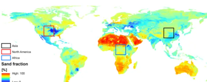
Figure 4.Example regions selected to evaluate the scaling variance loss from Warrick scaling at different spatial resolutions when neglecting the scaling variance. The background shows the sand fraction from SoilGrids1km.
Note that the Campbell approach is similar to the Brooks and Corey (1964) approach – the only difference is that the latter did not setθr=0 in the WRC. Also, Clapp and Hornberger (1978) did not considerθrin their equations.
2.5.2 Analysis of scaling variability for different spatial resolutions
In order to stress the importance of considering the sub-grid scaling information provided by the proposed method, the mean var(log10λˆi) is quantified for different spatial
resolutions. Three regions were analysed in more detail – namely regions in North America, central Africa and China/Mongolia consisting of 2048×2048 fine pixels from the SoilGrids1km database (see Fig. 4). For each of these larger regions a single parameter set ofαˆ andnˆis estimated by using Eq. (5). For each fine 1 km pixel the scaling parame-terλˆiis calculated according to Eq. (7). Different resolutions
of 2, 4, 8, 16, 32, 64, 128, 256, 512 and 1024 km were applied to the resulting map of λˆi. For each spatial resolution the
cell-specific scaling parameter is averaged (mean(log10λˆi)).
Finally, the variance of these averaged scaling parameters is calculated for the large regions. Herein we hypothesize that the variance of the scaling parameter is a function of spatial resolution.
This analysis uses the original SoilGrids1km spatial reso-lution as a reference. However, it has to be mentioned that the calculated scaling variability only refers to the information content of the SoilGrid 1 km reference, and does not neces-sarily provide the real soil scaling variability.
3 Results and discussion
Figure 5.Global map ofαˆ(a),nˆ(b),θs(c)and mean(log10(Ks))(d), as derived when using the SoilGrids1km data set as input to the Rosetta PTF (Schaap et al., 2001), at 0.25◦spatial resolution.
3.1 Global analysis
The resulting global hydraulic parametersα,ˆ n,ˆ θsas well as mean(log10Ks) are presented in Fig. 5. Parameterαˆ ranges between 0.0036 and 0.045 cm−1 with a global average of 0.0143 cm−1and shows a clear biogeographical or climatic related distribution. Relatively low values can be found mainly under boreal forests, but also in the North China
Figure 6.Global map of var(log10λˆi) calculated from SoilGrids1km data set and the Rosetta PTF (Schaap et al., 2001) for 0.25◦resolution.
Table 1.Variables stored in the final data set. The variablezindicates the soil depth, i.e.z∈ [0,5,15,30,60,100,200]cm.
Variable Units Explanation Variable name
Latitude Decimal degree Latitude in degrees north, Southern Hemisphere in negative numbers Latitude Longitude Decimal degree Longitude in degrees east, west of Greenwich in negative numbers Longitude ˆ
α cm−1 Fittedαatzcm depth for MvG parameterization alpha_fit_zcm
ˆ
n – Fittednatzcm depth for MvG parameterization n_fit_zcm
θs m3m−3 Meanθsatzcm depth for MvG parameterization mean_theta_s_zcm
θr m3m−3 Meanθratzcm depth for MvG parameterization mean_theta_r_zcm
L – Mean pore connectivity parameter atzcm depth for MvG parameterization mean_L_zcm
(mean(log10Ks)) cm d−1 Mean saturated hydraulic conductivity atzcm depth mean_Ks_zcm
var(log10λiˆ) – Scaling parameter variance atzcm depth var_scaling_zcm
Valid subpixels – Number of valid subpixels for calculating scaling statistics for thezcm soil depth valid_subpixels_zcm
in Australia. Smaller regions with highαˆ could be traced in Florida and the morainal plains of northern Europe and the Rocky Mountains. The global average ofnˆ is 1.547, with a range between 1.174 and 4.33 (–). The extreme highnˆ val-ues are found only in the non-alluvial regions of the Sahara and Rub’ al Khali (“Empty Quarter”, Arab Peninsula). The relatively high global average ofnˆis caused by the same ef-fect that caused the low αˆ average in the low bulk density of boreal top soils. Those soils typically are characterized by high organic carbon contents, behave quite differently in hydraulic sense compared to more mineral-dominated soils, and are rarely used to develop classical PTFs. Therefore, in-dependent of the aggregation or up-scaling approaches, more research is needed to adequately parameterize boreal soils by appropriate PTFs.
The global map of mean saturated hydraulic conductiv-ity (mean(log10Ks)) in Fig. 5 ranges between 0.174 and 3.105 with a global average of 1.784 (cm d−1). Low soil-saturated hydraulic conductivities are located in India, the Sahel, the Mediterranean, central Asia, the Levant and Iran, Texas, the US prairie regions, California and south-central Canada. Highest mean(log10Ks) are found in the Sahara and Rub’ al Khali, where sandy soils dominate, but also in the upper Amazon Basin (Marthews et al., 2014) and in cold cli-mates.
Figure 6 shows the global map of sub-grid scaling variance calculated from SoilGrids1km data set with a 0.25◦grid ref-erence. Global var(log10λˆi) ranges between∼0 and 1.574,
with an average value of 0.229. This shows that large re-gions, e.g. Siberia, East China, southern coastal provinces of Brazil and Mexico, are relatively homogeneous within in-dividual grid cells. The regions with particularly high sub-grid variability are typically transition zones of soils evolved from young sediments. Examples are the holocene morainal plains in northern Europe and Canada, as well as the slopes of high mountains areas of the Andes and Himalayas. Simi-larly, young deposits of large rivers such as the Amazon and the inner Congo Basin are characterized by high variability. These are the regions where the consideration of the sub-grid variability may have strong impacts on weather prediction and climate simulations.
Figure 7.PF curve after applying typical scaling or aggregation methods: by dominant USDA soil class and Clapp and Hornberger param-eters for the Brooks and Corey equation, by dominant USDA soil class and MvG equation, by averaging soil texture paramparam-eters and then applying ROSETTA PTFs, and by averaging MvG soil hydraulic parameters directly, for Lower Saxony (left) and North Rhine-Westphalia (right).
Figure 8.Retention curves for Lower Saxony (left) and North Rhine-Westphalia (right) calculated using different approaches. The coarse pixel fit is the result of the Warrick scaling approach, where (log10λˆi) was also estimated. Therefore,±1 SD(log10λˆi) could also be provided to identify the sub-grid uncertainty. Further retention curves were calculated by dominant USDA class (both for Brooks and Corey with Clapp and Hornberger and for MvG equation), by averaging texture and by averaging MvG parameters. Blue points indicateSeat standard hydraulic heads for each individual subpixel.
3.2 Example pixels
The detailed analysis of the WRC of two example model grid cells after applying a range of typical aggregation methods is shown in Fig. 7. This includes aggregation by averaging soil texture information, averaging MvG soil hydraulic parame-ters, and by selecting the dominant USDA soil class (both with MvG and Campbell equations). Averaging soil texture and averaging MvG parameters to a coarser grid caused dif-ferences in the WRC for Lower Saxony but showed nearly the same curve for North Rhine-Westphalia. The reasons why textural and MvG parameter averaging yielded the same ag-gregated WRC in North Rhine-Westphalia are unclear but
Figure 9.Hydraulic conductivity curves for Lower Saxony (left) and North Rhine-Westphalia (right). The coarse pixel fit is the result of the Warrick scaling approach, where (log10λˆ
i) was also estimated. Therefore,±1 SD(log10λˆi) could also be provided to identify the sub-grid uncertainty. Further hydraulic conductivity curves were calculated by dominant USDA class (both for Brooks and Corey with Clapp and Hornberger and for MvG equation), by averaging texture and by averaging MvG parameters. Blue points indicate log10(Kr) at standard hydraulic heads for each individual subpixel.
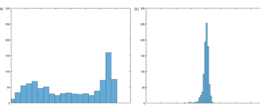
Figure 10.Histograms of the retention scaling parameter (log10λˆ
i) for Lower Saxony (left) and North Rhine-Westphalia (right).
Finally, the WRCs based on the different aggregation ap-proaches (dominant soil class, texture averaging, Warrick scaling) are presented in Fig. 8 for the two example regions. As can be seen, the effective saturation (Sei) calculated for
the 1 km sub-pixels at the standard heads of the head vector h (Eq. 3) (blue dots) reflects the natural variability in soil texture and corresponding soil hydraulic properties of the two example regions. This subscale variability is also ctured by the standard deviation of the Warrick scaling ap-proach, which is larger for Lower Saxony as compared to North Rhine-Westphalia. This indicates nicely that Warrick scaling is an appropriate approach to capture fine-scale vari-ability and to propagate the fine-scale uncertainty into the larger scale of interest.
A similar pattern of the different scaling methods can be also found for the HCCs presented in Fig. 9. By this Warrick
scaling approach, not only can large-scale modelling capture the right aggregated “mean” WRCs and HCCs but also the uncertainty can be taken into account by running the mod-els for the retention/hydraulic characteristics spanned by the variance of the scaling factor.
Figure 11.Retention scaling parameter variance var(log10λˆ
i) for different grid resolutions and regions of interest (North America, Africa and China; see also Fig. 4). (Left) absolute variance and (right) variance normalized as percentage of the maximum variance at 1 km original SoilGrids1km resolution.
3.3 Analysing scaling variability for different spatial resolutions
For the analysis of the scaling variability for different spa-tial resolutions the mean variance (var(log10λˆi)) was
calcu-lated for different grid resolutions and plotted in Fig. 11. For all three case sites (North America, Africa and China; see also Fig. 3) var(log10λˆi) decreased with decreasing spatial
resolution; the absolute scaling parameter variability of the Africa region is largest. This can be explained by the fact that the Sahel is prone to strong seasonal dry–wet cycles, which induces large variability in soil development (Da Costa et al., 2015). On the other hand, the relative decrease of vari-ance with coarser resolution for this region is comparable to the other ones (Fig. 11, right panel).
Interestingly,∼90 % of the variance is still maintained at 16 km grid size, ∼80% at 64 km, and ∼70 % at 128 km. Even at 256 km spatial resolution, more than 50 % of the variability is accounted for, but a diverging trend between the regions is detectable.
3.4 Inherent uncertainties
The use of PTFs and the practice of up-scaling of parame-ters from 1 km to grid scales where LSMs or related mod-els such as GCMs are applied; both introduce uncertainty which needs to be discussed. Here it is important to men-tion that the scaling variance var(log10λˆ
i) calculated with the
proposed approach denotes only the spatial sub-grid vari-ance from 1 km resolution of SoilGrids1km towards 0.25◦ resolution, but this implies no information about the specific uncertainties mentioned above. Moreover, we restricted the analysis to the mean predicted values of SoilGrids1km vari-ables such as texture and bulk density, but the full predic-tion uncertainty within a confidence interval could be used in an extended approach to estimate the soil hydraulic
prop-erty uncertainty. Another source of uncertainty is the use of the log-transform for scaling multiplier in Warrick scaling and averaging the saturated hydraulic conductivity using log transform. The applicability of a PFT to global scale may be limited for specific conditions, because the soil database used to estimate the transfer functions is often regionally lim-ited, so that the extrapolation to soils not included in the sta-tistical analysis introduces large uncertainty (e.g. for boreal soils). Finally, we aimed to provide a consistent data set and therefore derived the HCC from WRC rather than calculat-ing them independently. The new data set was developed and all calculations were made under the hypothesis that spatial variance of WRC and HCC scales with spatial resolution.
4 Data availability
The SoilGrids1km data set can be accessed at www.soilgrids. org.
5 Conclusions and outlook
us-ing Richards’ equation. In addition, the sub-grid variabil-ity of both WRC and HCC is assessed, which can be of use for model ensemble generation in climate and weather forecast models, or for down-/up-scaling approaches. The fi-nal global data set at 0.25◦spatial resolution is available at https://doi.org/10.1594/PANGAEA.870605.
The new data set is presented and analysed at the global scale and in more detail by two different individual pixels differing strongly in textural composition. In comparison to aggregation by using dominant USDA soil classes, averag-ing soil texture and averagaverag-ing soil hydraulic parameters, the curve fitting approach provides better estimates of coarse-scale water retention and conductivity curves and related pa-rameters. Moreover, the Warrick scaling provides an indica-tor of sub-grid variability, which is not available from the other methods mentioned above. For three regions different spatial resolutions were analysed according to their ability to represent the soil hydraulic variability of the original Soil-Grids database at 1 km resolution. For all regions a com-mon general loss of variability was observed, with losing ∼10 % of the variance at 16 km grid size,∼20 % at 64 km, and ∼30 % at 128 km. This has large implications for the application of global climate models. Process descriptions which are directly influenced by the hydraulic parameteriza-tion such as evaporaparameteriza-tion and infiltraparameteriza-tion may lose important information about extreme conditions when applying models at too coarse spatial resolution.
The presented analysis has been conducted on two-dimensional soil maps, without consideration of vertical re-lationships between soil layers or horizons. This approach can be easily extended towards a three-dimensional scaling that honours the vertical spatial dependency. A follow-up pa-per will assess the impact of this data set on water and energy fluxes at the soil surface for global simulations. Similarly, the effect of using other PTFs than Schaap et al. (2001) needs to be evaluated on the global scale as well as the uncertainties introduced during pedotransfer on the scaling parameteriza-tion. We plan to provide similar data sets for other PTFs, e.g. of Rawls and Brakensiek (1985), Wösten et al. (1999), Wey-nants et al. (2009) and Vereecken et al. (1989). A similar ap-proach is planned to provide parameters for the Brooks and Corey equation.
Competing interests. The authors declare that they have no con-flict of interest.
Acknowledgements. This study was supported by the Helmholtz Alliance on “Remote Sensing and Earth System Dynamics”.
Edited by: Giuseppe M. R. Manzella Reviewed by: two anonymous referees
References
Ahuja, L. R., Naney, J. W., and Nielsen, D. R.: Scaling Soil-Water Properties and Infiltration Modeling, Soil Sci. Soc. A. J., 48, 970–973, 1984.
Ballabio, C., Panagos, P., and Monatanarella, L.: Map-ping topsoil physical properties at European scale us-ing the LUCAS database, Geoderma, 261, 110–123, https://doi.org/10.1016/j.geoderma.2015.07.006, 2016.
Balsamo, G., Albergel, C., Beljaars, A., Boussetta, S., Brun, E., Cloke, H., Dee, D., Dutra, E., Muñoz-Sabater, J., Pappen-berger, F., de Rosnay, P., Stockdale, T., and Vitart, F.: ERA-Interim/Land: a global land surface reanalysis data set, Hydrol. Earth Syst. Sci., 19, 389–407, https://doi.org/10.5194/hess-19-389-2015, 2015.
Bauer, J., Weihermuller, L., Huisman, J. A., Herbst, M., Graf, A., Sequaris, J. M., and Vereecken, H.: Inverse determination of heterotrophic soil respiration response to temperature and water content under field conditions, Biogeochemistry, 108, 119–134, https://doi.org/10.1007/s10533-011-9583-1, 2012.
Best, M. J., Pryor, M., Clark, D. B., Rooney, G. G., Essery, R. L. H., Ménard, C. B., Edwards, J. M., Hendry, M. A., Porson, A., Gedney, N., Mercado, L. M., Sitch, S., Blyth, E., Boucher, O., Cox, P. M., Grimmond, C. S. B., and Harding, R. J.: The Joint UK Land Environment Simulator (JULES), model description – Part 1: Energy and water fluxes, Geosci. Model Dev., 4, 677–699, https://doi.org/10.5194/gmd-4-677-2011, 2011.
Bouma, J.: Using Soil Survey Data for Quantitative Land Evalu-ation, in: Advances in Soil Science, edited by: Stewart, B. A., Springer US, New York, NY, 177–213, 1989.
Brooks, R. J. and Corey, A. T.: Hydraulic properties of porous me-dia, Colorado State University Fort Collins, CO, USA, Hydrol-ogy Papers, 3, 37 pp., 1964.
Cale, W. G., Oneill, R. V., and Gardner, R. H.: Aggregation Error in Non-Linear Ecological Models, J. Theor. Biol., 100, 539–550, 1983.
Campbell, G. S.: A Simple Method for Determining Unsaturated Conductivity From Moisture Retention Data, Soil Sci., 117, 311– 314, 1974.
Clapp, R. B. and Hornberger, G. M.: Empirical Equations for Some Soil Hydraulic-Properties, Water Resour. Res., 14, 601– 604, 1978.
Clausnitzer, V., Hopmans, J. W., and Nielsen, D. R.: Simultane-ous Scaling of Soil-Water Retention and Hydraulic Conductivity Curves, Water Resour. Res., 28, 19–31, 1992.
Da Costa, P. Y. D., Nguetnkam, J. P., Mvoubou, C. M., Togbe, K. A., Ettien, J. B., and Yao-Kouame, A.: Old landscapes, pre-weathered materials, and pedogenesis in tropical Africa: How can the time factor of soil formation be assessed in these re-gions?, Quatern. Int, 376, 47–74, 2015.
Dimitrov, M., Vanderborght, J., Kostov, K. G., Jadoon, K. Z., Weihermuller, L., Jackson, T. J., Bindlish, R., Pachepsky, Y., Schwank, M., and Vereecken, H.: Soil Hydraulic Parameters and Surface Soil Moisture of a Tilled Bare Soil Plot Inversely De-rived from L-Band Brightness Temperatures, Vadose Zone J., 13, 1, https://doi.org/10.2136/vzj2013.04.0075, 2014.
boundary-layer development, Bound.-Lay. Meteorol., 70, 369– 383, https://doi.org/10.1007/bf00713776, 1994.
Fallico, C., Tarquis, A. M., De Bartolo, S., and Veltri, M.: Scaling analysis of water retention curves for unsaturated sandy loam soils by using fractal geometry, Eur. J. Soil Sci., 61, 425–436, 2010.
Fang, Z. F., Bogena, H., Kollet, S., and Vereecken, H.: Scale depen-dent parameterization of soil hydraulic conductivity in 3D sim-ulation of hydrological processes in a forested headwater catch-ment, J. Hydrol., 536, 365–375, 2016.
Hendrayanto, Kosugi, K., and Mizuyama, T.: Scaling hydraulic properties of forest soils, Hydrol. Process., 14, 521–538, 2000. Hengl, T., de Jesus, J. M., MacMillan, R. A., Batjes, N. H., and
Heuvelink, G. B. M.: SoilGrids1km – Global Soil Informa-tion Based on Automated Mapping, PLoS ONE, 9, e114788, https://doi.org/10.1371/journal.pone.0114788, 2014.
Hoffmann, H., Zhao, G., Asseng, S., Bindi, M., Biernath, C., Con-stantin, J., Coucheney, E., Dechow, R., Doro, L., Eckersten, H., Gaiser, T., Grosz, B., Heinlein, F., Kassie, B. T., Kerse-baum, K. C., Klein, C., Kuhnert, M., Lewan, E., Moriondo, M., Nendel, C., Priesack, E., Raynal, H., Roggero, P. P., Rotter, R. P., Siebert, S., Specka, X., Tao, F. L., Teixeira, E., Trombi, G., Wallach, D., Weihermuller, L., Yeluripati, J., and Ewert, F.: Impact of Spatial Soil and Climate Input Data Aggrega-tion on Regional Yield SimulaAggrega-tions, PLoS ONE, 11, e0151782, https://doi.org/10.1371/journal.pone.0151782, 2016.
Jadoon, K. Z., Weihermuller, L., Scharnagl, B., Kowalsky, M. B., Bechtold, M., Hubbard, S. S., Vereecken, H., and Lam-bot, S.: Estimation of Soil Hydraulic Parameters in the Field by Integrated Hydrogeophysical Inversion of Time-Lapse Ground-Penetrating Radar Data, Vadose Zone J., 11, 4, https://doi.org/10.2136/vzj2011.0177, 2012.
Jana, R. B. and Mohanty, B. P.: Enhancing PTFs with remotely sensed data for multi-scale soil water retention estimation, J. Hy-drol., 399, 201–211, 2011.
Kuhnert, M., Yeluripati, J., Smith, P., Hoffmann, H., van Oijen, M., Constantin, J., Coucheney, E., Dechow, R., Eckersten, H., Gaiser, T., Grosz, B., Haas, E., Kersebaum, K.-C., Kiese, R., Klatt, S., Lewan, E., Nendel, C., Raynal, H., Sosa, C., Specka, X., Teixeira, E., Wang, E., Weihermüller, L., Zhao, G., Zhao, Z., Ogle, S., and Ewert, F.: Impact analysis of climate data aggregation at different spatial scales on simulated net pri-mary productivity for croplands, Eur. J. Agron., 88, 41–52, https://doi.org/10.1016/j.eja.2016.06.005, 2016.
Liang, X., Lettenmaier, D. P., Wood, E. F., and Burges, S. J.: A Simple Hydrologically Based Model of Land-Surface Water and Energy Fluxes for General-Circulation Models, J. Geophys. Res., 99, 14415–14428, 1994.
Liao, K., Xu, S., Wu, J., and Zhu, Q.: Uncertainty analysis for large-scale prediction of the van Genuchten soil-water retention param-eters with pedotransfer functions, Soil Res., 52, 431–442, 2014. Marquardt, D. W.: An Algorithm for Least-Squares Estimation of
Nonlinear Parameters, J. Soc. Ind. Appl. Math., 11, 431–441, 1963.
Marthews, T. R., Quesada, C. A., Galbraith, D. R., Malhi, Y., Mullins, C. E., Hodnett, M. G., and Dharssi, I.: High-resolution hydraulic parameter maps for surface soils in tropical South America, Geosci. Model Dev., 7, 711–723, https://doi.org/10.5194/gmd-7-711-2014, 2014.
Millan, H. and Gonzalez-Posada, M.: Modelling soil water retention scaling. Comparison of a classical fractal model with a piecewise approach, Geoderma, 125, 25–38, 2005.
Miller, E. E. and Miller, R. D.: Physical Theory for Capillary Flow Phenomena, J. Appl. Phys., 27, 324–332, 1956.
Montzka, C., Moradkhani, H., Weihermüller, L., Hendricks Franssen, H.-J., Canty, M., and Vereecken, H.: Hydraulic pa-rameter estimation by remotely-sensed top soil moisture ob-servations with the particle filter, J. Hydrol., 399, 410–421, https://doi.org/10.1016/j.jhydrol.2011.01.020, 2011.
Ngo-Duc, T., Laval, K., Ramillien, G., Polcher, J., and Cazenave, A.: Validation of the land water storage simulated by Organ-ising Carbon and Hydrology in Dynamic Ecosystems (OR-CHIDEE) with Gravity Recovery and Climate Experiment (GRACE) data, Water Resources Resour. Res., 43, W04427, https://doi.org/10.1029/2006WR004941, 2007.
Niu, G. Y., Yang, Z. L., Mitchell, K. E., Chen, F., Ek, M. B., Barlage, M., Kumar, A., Manning, K., Niyogi, D., Rosero, E., Tewari, M., and Xia, Y. L.: The community Noah land surface model with multiparameterization options (Noah-MP): 1. Model description and evaluation with local-scale measurements, J. Geophys. Res., 116, D12109, https://doi.org/10.1029/2010JD015139, 2011 Oleson, K. W., Niu, G. Y., Yang, Z. L., Lawrence, D. M.,
Thornton, P. E., Lawrence, P. J., Stöckli, R., Dickinson, R. E., Bonan, G. B., Levis, S., Dai, A., and Qian, T.: Im-provements to the Community Land Model and their impact on the hydrological cycle, J. Geophys. Res., 113, G01021, https://doi.org/10.1029/2007JG000563, 2008.
Pachepsky, Y. A., Shcherbakov, R. A., and Korsunskaya, L. P.: Scal-ing of Soil-Water Retention UsScal-ing a Fractal Model, Soil Sci., 159, 99–104, 1995.
Pierce, L. L. and Running, S. W.: The Effects of Aggregating Sub-grid Land-Surface Variation on Large-Scale Estimates of Net Pri-mary Production, Landscape Ecol., 10, 239–253, 1995. Rastetter, E. B., King, A. W., Cosby, B. J., Hornberger, G. M.,
Oneill, R. V., and Hobbie, J. E.: Aggregating Fine-Scale Eco-logical Knowledge to Model Coarser-Scale Attributes of Ecosys-tems, Ecol. Appl., 2, 55–70, 1992.
Rawls, W. J. and Brakensiek, D. L.: Prediction of soil water prop-erties for hydrologic modelling, American Society of Civil Engi-neers, 293–299, 1985.
Reynolds, C. A., Jackson, T. J., and Rawls, W. J.: Estimating soil water-holding capacities by linking the Food and Agriculture Or-ganization soil map of the world with global pedon databases and continuous pedotransfer functions, Water Resour. Res., 36, 3653–3662, 2000.
Rodell, M., Houser, P. R., Jambor, U., Gottschalck, J., Mitchell, K., Meng, C. J., Arsenault, K., Cosgrove, B., Radakovich, J., Bosilovich, M., Entin, J. K., Walker, J. P., Lohmann, D., and Toll, D.: The global land data assimilation system, B. Am. Meteorol. Soc., 85, 381–394, 2004.
Russo, D. and Bresler, E.: Scaling Soil Hydraulic-Properties of a Heterogeneous Field, Soil Sci. Soc. Am. J., 44, 681–684, 1980. Schaap, M. G., Leij, F. J., and van Genuchten, M. T.: ROSETTA: a
computer program for estimating soil hydraulic parameters with hierarchical pedotransfer functions, J. Hydrol., 251, 163–176, 2001.
investigat-ing the effect of different prior distributions of the soil hy-draulic parameters, Hydrol. Earth Syst. Sci., 15, 3043–3059, https://doi.org/10.5194/hess-15-3043-2011, 2011.
Scheinost, A. C., Sinowski, W., and Auerswald, K.: Regionaliza-tion of soil water retenRegionaliza-tion curves in a highly variable soilscape. 1. Developing a new pedotransfer function, Geoderma, 78, 129– 143, 1997.
Shu, Q. S., Liu, Z. X., and Si, B. C.: Characterizing Scale- and Location-Dependent Correlation of Water Retention Parameters with Soil Physical Properties Using Wavelet Techniques, J. Env-iron. Qual., 37, 2284–2292, 2008.
Simmons, C. S., Nielsen, D. R., and Biggar, J. W.: Scaling of Field-Measured Soil-Water Properties, Hilgardia, 47, 77–173, 1979. Tillotson, P. M. and Nielsen, D. R.: Scale Factors in Soil Science,
Soil Sci. Soc. Am. J., 48, 953–959, 1984.
Toth, B., Weynants, M., Nemes, A., Mako, A., Bilas, G., and Toth, G.: New generation of hydraulic pedotransfer functions for Eu-rope, Eur. J. Soil Sci., 66, 226–238, 2015.
Toth, G., Jones, A., and Montanarella, L.: LUCAS Topsoil Survey. Methodology, data and results, Publications Office of the Euro-pean Union, Luxembourg, 2013.
Tuli, A., Kosugi, K., and Hopmans, J. W.: Simultaneous scaling of soil water retention and unsaturated hydraulic conductivity func-tions assuming lognormal pore-size distribution, Adv. Water Re-sour., 24, 677–688, 2001.
van Dam, J. C., Groenendijk, P., Hendriks, R. F. A., and Kroes, J. G.: Advances of modeling water flow in variably saturated soils with SWAP, Vadose Zone J., 7, 640–653, 2008.
Van Engelen, V. and Dijkshoorn, J.: Global and National Soils and Terrain Digital Databases (SOTER), Procedures Manual, version 2.0, Wageningen, The Netherlands, 192 pp., 2012.
van Genuchten, M. T.: A Closed Form Equation for Predicting the Hydraulic Conductivity of Unsaturated Soils, Soil Sci. Soc. Am. J., 44, 892–898, 1980.
Vereecken, H., Maes, J., Feyen, J., and Darius, P.: Estimating the Soil-Moisture Retention Characteristic from Texture, Bulk-Density, and Carbon Content, Soil Sci., 148, 389–403, 1989. Vereecken, H., Weynants, M., Javaux, M., Pachepsky, Y., Schaap,
M. G., and van Genuchten, M. T.: Using Pedotransfer Functions to Estimate the van Genuchten-Mualem Soil Hydraulic Proper-ties: A Review, Vadose Zone J., 9, 795–820, 2010.
Vereecken, H., Schnepf, A., Hopmans, J. W., Javaux, M., Or, D., Roose, T., Vanderborght, J., Young, M. H., Amelung, W., Aitkenhead, M., Allison, S. D., Assouline, S., Baveye, P., Berli, M., Brüggemann, N., Finke, P., Flury, M., Gaiser, T., Gov-ers, G., Ghezzehei, T., Hallett, P., Hendricks Franssen, H. J., Heppell, J., Horn, R., Huisman, J. A., Jacques, D., Jonard, F., Kollet, S., Lafolie, F., Lamorski, K., Leitner, D., McBrat-ney, A., Minasny, B., Montzka, C., Nowak, W., Pachepsky, Y., Padarian, J., Romano, N., Roth, K., Rothfuss, Y., Rowe, E. C., Schwen, A., Šim˚unek, J., Tiktak, A., Van Dam, J., van der Zee, S. E. A. T. M., Vogel, H. J., Vrugt, J. A., Wöh-ling, T., and Young, I. M.: Modeling Soil Processes: Review, Key Challenges, and New Perspectives, Vadose Zone J., 15, 5, https://doi.org/10.2136/vzj2015.09.0131, 2016.
Verhoef, A. and Egea, G.: Modeling plant transpiration under lim-ited soil water: Comparison of different plant and soil hydraulic parameterizations and preliminary implications for their use in land surface models, Agr. Forest Meteorol., 191, 22–32, 2014. Walko, R. L. and Avissar, R.: The Ocean-Land-Atmosphere Model
(OLAM). Part I: Shallow-Water Tests, Mon. Weather Rev., 136, 4033–4044, 2008.
Walters, D. N., Williams, K. D., Boutle, I. A., Bushell, A. C., Ed-wards, J. M., Field, P. R., Lock, A. P., Morcrette, C. J., Strat-ton, R. A., Wilkinson, J. M., Willett, M. R., Bellouin, N., Bodas-Salcedo, A., Brooks, M. E., Copsey, D., Earnshaw, P. D., Hardi-man, S. C., Harris, C. M., Levine, R. C., MacLachlan, C., Man-ners, J. C., Martin, G. M., Milton, S. F., Palmer, M. D., Roberts, M. J., Rodríguez, J. M., Tennant, W. J., and Vidale, P. L.: The Met Office Unified Model Global Atmosphere 4.0 and JULES Global Land 4.0 configurations, Geosci. Model Dev., 7, 361–386, https://doi.org/10.5194/gmd-7-361-2014, 2014.
Wang, Z. Y., Shu, Q. S., Liu, Z. X., and Si, B. C.: Scaling analysis of soil water retention parameters and physical properties of a Chinese agricultural soil, Aust. J. Soil Res., 47, 821–827, 2009. Warrick, A. W., Mullen, G. J., and Nielsen, D. R.: Scaling
Field-Measured Soil Hydraulic-Properties Using a Similar Media Con-cept, Water Resour. Res., 13, 355–362, 1977.
Weynants, M., Vereecken, H., and Javaux, M.: Revisiting Vereecken Pedotransfer Functions: Introducing a Closed-Form Hydraulic Model, Vadose Zone J., 8, 86–95, 2009.
Wösten, J. H. M., Lilly, A., Nemes, A., and Le Bas, C.: Develop-ment and use of a database of hydraulic properties of European soils, Geoderma, 90, 169–185, 1999.
Xue, Y. K., Zeng, F. J., and Schlosser, C. A.: SSiB and its sensitivity to soil properties – A case study using HAPEX-Mobilhy data, Global Planet Change, 13, 183–194, 1996.
Zeleke, T. B. and Si, B. C.: Wavelet-based multifractal analysis of field scale variability in soil water retention, Water Resour. Res., 43, W07446, https://doi.org/10.1029/2006WR004957, 2007. Zhu, J. T. and Mohanty, B. P.: Spatial Averaging of van Genuchten