https://doi.org/10.5194/gmd-10-2651-2017 © Author(s) 2017. This work is distributed under the Creative Commons Attribution 3.0 License.
Global evaluation of gross primary productivity in the JULES land
surface model v3.4.1
Darren Slevin1, Simon F. B. Tett1, Jean-François Exbrayat1,2, A. Anthony Bloom1,2,3, and Mathew Williams1,2
1School of GeoSciences, The University of Edinburgh, Crew Building, Alexander Crum Brown Road, Edinburgh,
EH9 3FF, UK
2National Centre for Earth Observation, The University of Edinburgh, Crew Building, Alexander Crum Brown Road,
Edinburgh, EH9 3FF, UK
3Jet Propulsion Laboratory, California Institute of Technology, Pasadena, CA 91109, USA Correspondence to:Darren Slevin ([email protected])
Received: 26 August 2016 – Discussion started: 21 September 2016 Revised: 18 May 2017 – Accepted: 2 June 2017 – Published: 11 July 2017
Abstract.This study evaluates the ability of the JULES land surface model (LSM) to simulate gross primary productivity (GPP) on regional and global scales for 2001–2010. Model simulations, performed at various spatial resolutions and driven with a variety of meteorological datasets (WFDEI-GPCC, WFDEI-CRU and PRINCETON), were compared to the MODIS GPP product, spatially gridded estimates of upscaled GPP from the FLUXNET network (FLUXNET-MTE) and the CARDAMOM terrestrial carbon cycle analy-sis. Firstly, when JULES was driven with the WFDEI-GPCC dataset (at 0.5◦×0.5◦ spatial resolution), the annual aver-age global GPP simulated by JULES for 2001–2010 was higher than the observation-based estimates (MODIS and FLUXNET-MTE), by 25 and 8 %, respectively, and CAR-DAMOM estimates by 23 %. JULES was able to simulate the standard deviation of monthly GPP fluxes compared to CARDAMOM and the observation-based estimates on global scales. Secondly, GPP simulated by JULES for var-ious biomes (forests, grasslands and shrubs) on global and regional scales were compared. Differences among JULES, MODIS, FLUXNET-MTE and CARDAMOM on global scales were due to differences in simulated GPP in the trop-ics. Thirdly, it was shown that spatial resolution (0.5◦×0.5◦, 1◦×1◦and 2◦×2◦) had little impact on simulated GPP on these large scales, with global GPP ranging from 140 to 142 PgC year−1. Finally, the sensitivity of JULES to mete-orological driving data, a major source of model uncertainty, was examined. Estimates of annual average global GPP were higher when JULES was driven with the PRINCETON
meteorological dataset than when driven with the WFDEI-GPCC dataset by 3 PgC year−1. On regional scales, differ-ences between the two were observed, with the WFDEI-GPCC-driven model simulations estimating higher GPP in the tropics (5◦N–5◦S) and the PRINCETON-driven model simulations estimating higher GPP in the extratropics (30– 60◦N).
1 Introduction
The land surface is an important component of the climate system, providing the lower boundary for the atmosphere and exchanging energy, water and carbon (C) with the atmo-sphere (Pielke et al., 1998; Pitman, 2003; Seneviratne and Stöckli, 2008). It also controls the partitioning of available energy (into latent and sensible heat) and water (into evap-oration and runoff) at the surface (Bonan, 2008). Changes in the land surface due to human activities, such as those from tropical deforestation, can influence climate on vari-ous timescales and spatial scales, and since the land surface is the location of the terrestrial C cycle, its ability to act as a C source or sink can influence atmospheric CO2
concen-trations (Le Quéré et al., 2009; Pan et al., 2011; Le Quéré et al., 2013; Tian et al., 2016). The reduced ability of the land surface to absorb increased anthropogenic CO2emissions in
Friedlingstein et al., 2014; Sitch et al., 2015). Friedlingstein et al. (2006) and Friedlingstein et al. (2014) have suggested that a major source of model uncertainty is the land C cycle which can affect the ability of Earth system models (ESMs; also known as coupled carbon-cycle–climate models) to re-liably simulate future atmospheric CO2 concentrations and
climate (Dalmonech et al., 2014).
Plants fix CO2 as organic compounds through
photosyn-thesis on the leaf scale, and gross primary productivity (GPP) is the total amount of C used in photosynthesis by plants at the ecosystem level (Beer et al., 2010; Chapin III et al., 2012). Photosynthesis on the leaf and canopy scale vary in response to changes in climate (temperature, precipitation, humidity and downward radiation fluxes) and nutrient avail-ability (Anav et al., 2015). Terrestrial GPP is an important (and the largest) C flux since it drives several ecosystem functions such as respiration and growth (Beer et al., 2010). GPP contributes to the production of food, fibre and wood for humans and, along with respiration, is one of the major pro-cesses controlling the exchange of CO2between the land and
atmosphere (Beer et al., 2010). It also plays an important role in the global C cycle, helping terrestrial ecosystems to par-tially offset anthropogenic CO2 emissions (Janssens et al.,
2003; Cox and Jones, 2008; Battin et al., 2009; Anav et al., 2015)
However, on the global scale, there are no direct mea-surements of GPP (Anav et al., 2015). Global estimates of GPP exist, but are not solely based on measurements and, therefore, large uncertainties exist in these estimates (Anav et al., 2015). In LSMs, the correct simulation of GPP is im-portant since errors in its calculation can propagate through the model and affect biomass and other flux calculations, such as net ecosystem exchange (NEE; Schaefer et al., 2012). The correct representation of leaf-level stomatal conductance influences GPP and transpiration, and errors in GPP can also introduce errors into simulated latent and sensible heat fluxes.
Land surface models (LSMs) have become considerably more complex since the simple “bucket” model of Manabe (1969). Deardorff (1978) developed a model which could simulate temperature and moisture for two soil layers and included a vegetation layer. Sellers et al. (1986) built on the work of Deardorff (1978) by developing a globally ap-plicable LSM. Foley et al. (1996) incorporated vegetation dynamics into an LSM. These developments have led to LSMs which can realistically represent complex vegetation responses to meteorology, the climate effect of snow and bio-geochemical processes (Pitman, 2003; van den Hurk et al., 2011). Therefore, as LSMs become more complex, their ac-curacy must be evaluated.
The Joint UK Land Environment Simulator (JULES) has been evaluated on various scales: point (Blyth et al., 2010, 2011; Slevin et al., 2015; Ménard et al., 2015), regional (Galbraith et al., 2010; Burke et al., 2013; Chadburn et al., 2015) and globally as part of model-intercomparison studies
(Anav et al., 2015; Sitch et al., 2015). Evaluating simulated GPP on a range of scales and its sensitivity to spatial reso-lution and meteorological data is essential for informing fu-ture model developments. In this paper, we do this using two observation-based datasets (FLUXNET-MTE and MODIS) and the Carbon Data Model Framework (Bloom et al., 2016, CARDAMOM).
In this study, the ability of JULES version 3.4.1 to sim-ulate global and regional fluxes of GPP for various biomes, at various spatial resolutions and using different meteorolog-ical data to drive the model, is evaluated. In particular, the following research questions are addressed:
– How do estimates of global GPP compare to those from the observation-based datasets and the CARDAMOM framework? Can JULES capture interannual variability of GPP on the global scale?
– How does JULES GPP compare for various biomes on the global and regional scales?
– How sensitive are fluxes of GPP to the spatial resolution of the model?
– Is the meteorological dataset used to drive the model important on the global scale?
2 Methods and model 2.1 Model description
JULES is driven by the downward shortwave and long-wave radiation fluxes, rainfall and snowfall rates, surface air temperature, wind speed, surface pressure, and specific humidity. The downward shortwave and longwave radiation fluxes play an important role in the surface energy balance, where the downwelling radiation fluxes must equal the out-going fluxes of sensible heat, latent heat, ground flux, re-flected shortwave radiation and upwelling thermal energy, and the calculation of photosynthesis (Best et al., 2011; Clark et al., 2011). GPP is the total C uptake by plants in pho-tosynthesis on the canopy scale with potential (without wa-ter and ozone stress) leaf-level photosynthesis calculated as the smoothed minimum of three limiting rates: (1) Rubisco-limited rate (determined using surface air temperature and atmospheric CO2concentrations), (2) light-limited rate
(de-termined using downward shortwave radiation) and (3) rate of transport of photosynthetic products (C3plants) and
PEP-Carboxylase limitation (C4plants; determined using surface
air temperature and pressure; Clark et al., 2011). Soil mois-ture stress is taken into account when calculating leaf-level photosynthesis by multiplying the potential leaf-level photo-synthesis by a soil moisture factor (determined using mean soil moisture concentration in the root zone).
In JULES, there are two options available for radiation in-terception and the scaling of photosynthesis from leaf level to canopy level: (i) big leaf approach and (ii) multi-layer ap-proach. For all model simulations performed in this study, the multi-layer approach was used, which takes into account the vertical gradient of canopy photosynthetic capacity (de-creasing leaf nitrogen from top to bottom of canopy) and includes light inhibition of leaf respiration (Option 4 in Ta-ble 3 of Clark et al., 2011). Canopy-scale fluxes are estimated to be the sum of the leaf-level fluxes in each canopy layer, scaled by leaf area. LAI (leaf area index) is calculated for each canopy level (default number is 10), with a maximum LAI prescribed for each PFT.
Phenology (bud burst and leaf senescence) in JULES is usually updated once per day by multiplying the annual max-imum LAI by a scaling factor (calculated using accumulated temperature-dependent leaf turnover rates). For each PFT, the C fluxes are calculated using a coupled photosynthesis– stomatal conductance model on each model timestep (typi-cally 30 to 60 min; Cox et al., 1998). These fluxes are then time-averaged (usually every 10 days) before being passed to TRIFFID (Top-down Representation of Interactive Foliage and Flora Including Dynamics), JULES’ dynamic global vegetation model, which updates the vegetation distribution, based on the net C available to it and competition with other vegetation types, and soil C in each model grid box on a longer timestep (usually every 10 days; Cox, 2001). Clark et al. (2011) and Best et al. (2011) contain a more detailed description of JULES.
2.2 Experimental design
Offline simulations of GPP were performed on the global scale for the 2001–2010 period using various meteorological datasets and spatial resolutions (Table 1). A general overview is provided of how sensitive JULES GPP is to the meteoro-logical dataset used on global scales rather than for each me-teorological variable. By analysing the model sensitivity to each meteorological dataset, different analyses of the global climate are compared, and therefore a multi-factor analysis of combined changes in meteorological variables can be per-formed. The land cover was kept constant at the year 2000 values (Loveland et al., 2000) and annual atmospheric CO2
concentrations were varied as in the historical record. The 2001–2010 time period was used to due to the availability of multiple global meteorological and GPP datasets for this pe-riod. JULES is compared against FLUXNET-MTE, MODIS and CARDAMOM GPP.
Prior to performing the global-scale model simulations, the soil moisture was brought to equilibrium using a 40-year global spin-up by cycling 10 40-years of meteorological data (1979–1989) twice and 10 years of meteorological data (1989–1999) twice (in equilibrium mode), followed by a 12 year spin-up by cycling 12 years of meteorological data (1999–2010) once (in dynamical mode). Clark et al. (2011) contains more information on spinning up the soil C pools. 2.3 Data
The datasets used in this study include those used as input to JULES (soil, vegetation and meteorological data) and the benchmarking data. The soil dataset used was the Harmo-nized World Soil Database version 1.2 (Nachtergaele et al., 2012, HWSD) and contains soil property data such as soil texture fractions, water storage capacity, soil depth and pH (Nachtergaele et al., 2012). In this study, the soil texture frac-tions (percentage of sand, silt and clay) were used to calcu-late the soil thermal and hydraulic conductivity parameters listed in Table 3 of Best et al. (2011). The land cover clas-sification scheme used for specifying the PFT fractions for each model grid box on the global scale was Global Land Cover Characterization database version 2.0 (Loveland et al., 2000, http://edc2.usgs.gov/glcc/glcc.php). Two meteorologi-cal datasets were used to drive the model offline (i.e. run sep-arately from its host Earth system model) on global scales: WFDEI (Weedon et al., 2014) and PRINCETON (Sheffield et al., 2006).
Table 1.Types of global-scale model simulations performed.
Model Meteorological Spatial Grid simulations forcing resolution dimensions∗ JULES-WFDEI-GPCC WFDEI-GPCC 0.5◦×0.5◦ 720×360 JULES-WFDEI-CRU WFDEI-CRU 0.5◦×0.5◦ 720×360 JULES-WFDEI-GPCC-1degree WFDEI-GPCC 1◦×1◦ 360×180 JULES-PRINCETON PRINCETON 1◦×1◦ 360×180 JULES-WFDEI-GPCC-2degree WFDEI-GPCC 2◦×2◦ 180×90
∗Grid dimensions are given as the number of grid boxes in the longitudinal direction by the number of grid
boxes in the latitudinal direction.
Carbon Data Model Framework (Bloom et al., 2016, CAR-DAMOM). These global gridded estimates of GPP provide a means of evaluating LSMs on large scales (Jung et al., 2009, 2010; Beer et al., 2010; Zhao and Running, 2010; Bonan et al., 2011; Lei et al., 2014).
2.3.1 Forcing data
As part of the EMBRACE EU FP7 programme (http:// www.embrace-project.eu/), the WATCH forcing data (WFD) methodology was applied to the ERA-Interim reanalysis data for the 1979–2013 period to generate the WFDEI meteoro-logical forcing data (Weedon et al., 2014). As for the WFD, WFDEI has two precipitation products, corrected using ei-ther CRU (Climate Research Unit at the University of East Anglia) or GPCC (Global Precipitation Climatology Cen-tre) precipitation totals (Weedon et al., 2014) and are re-ferred to as WFDEI-CRU and WFDEI-GPCC, respectively. The GPCC data product is a gridded gauged precipitation dataset and provides a higher resolution dataset (i.e. better station coverage, particularly at high latitudes, and especially for the end of the 20th century) than the CRU precipitation totals (Weedon et al., 2014). The WFDEI dataset consists of 3-hourly, regularly gridded data at half-degree (0.5◦×0.5◦) spatial resolution and is only available for land points includ-ing Antarctica. The dataset contains the followinclud-ing meteoro-logical variables: downward shortwave and longwave radia-tion fluxes (W m−2), rainfall rate (kg m−2s−1), snowfall rate (kg m−2s−1), 2 m temperature (K), 10 m wind speed (m s−1), surface pressure (Pa), and 2 m specific humidity (kg kg−1).
The PRINCETON dataset is a global 62-year near-surface meteorological dataset used for driving land surface mod-els and was created by Princeton University’s Terrestrial Hydrology Group (Sheffield et al., 2006, http://hydrology. princeton.edu/home.php). The PRINCETON dataset consists of 3-hourly, regularly gridded data at 1-degree (1◦×1◦) spa-tial resolution for the 1948–2010 period and is only available for land points excluding Antarctica. The dataset contains the same meteorological variables as WFDEI with the exception of rainfall and snowfall rates summed as total precipitation (kg m−2s−1).
2.3.2 Benchmarking data
The upscaled FLUXNET GPP (hereafter referred to as FLUXNET-MTE) was derived using a model tree ensem-ble (MTE) approach, a type of machine learning technique that can be trained to predict land–atmosphere fluxes (Jung et al., 2009). Based on observed meteorological data, land cover data and remotely sensed vegetation properties (frac-tion of absorbed photosynthetic active radia(frac-tion), the upscal-ing principle can predict estimates of C fluxes at FLUXNET sites with available quality-filtered flux data, and the trained model is then applied spatially using grids of the input data (Jung et al., 2009, 2011). However, these machine learn-ing algorithms are typically data-limited due to the quan-tity, quality and representativeness of the training dataset (Jung et al., 2009). There are two upscaled FLUXNET GPP datasets available depending on the flux partitioning method used to separate net ecosystem exchange (NEE) of CO2into
GPP and terrestrial ecosystem respiration (TER; Reichstein et al., 2005; Lasslop et al., 2010). In this study, GPP based on the work by Reichstein et al. (2005) was used (this is the flux partitioning method used by the FLUXNET network). How-ever, differences between the two upscaled FLUXNET GPP datasets are small. FLUXNET-MTE is a 0.5◦×0.5◦spatial and monthly temporal resolution dataset for the 1982–2011 period and is available from the Max Planck Institute for Biogeochemistry Data Portal (https://www.bgc-jena.mpg.de/ geodb/projects/Home.php).
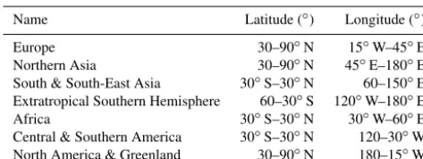
Table 2.List of regions used. Only land grid points are used in the analysis.
Name Latitude (◦) Longitude (◦)
Europe 30–90◦N 15◦W–45◦E
Northern Asia 30–90◦N 45◦E–180◦E
South & South-East Asia 30◦S–30◦N 60–150◦E Extratropical Southern Hemisphere 60–30◦S 120◦W–180◦E
Africa 30◦S–30◦N 30◦W–60◦E
Central & Southern America 30◦S–30◦N 120–30◦W North America & Greenland 30–90◦N 180–15◦W
coarse resolution meteorological data, temporal infilling of cloud-contaminated MOD15A2 LAI/FPAR data and mod-ification of BPLUT (Biome Property Look-Up Table) pa-rameters based on observed GPP from flux tower measure-ments in order to create an improved MOD17 GPP product (Zhao et al., 2005). The global monthly MODIS GPP (ver-sion 55) dataset at 0.05◦×0.05◦ spatial resolution for the 2001–2010 period was downloaded from ftp://ftp.ntsg.umt. edu/pub/MODIS/NTSG_Products/. For the purposes of this study, the data were regridded to 0.5◦×0.5◦ spatial reso-lution using the first-order conservative remapping function (remapcon) of the Climate Data Operators (CDO) software package (https://code.zmaw.de/projects/cdo).
The Carbon Data Model Framework (CARDAMOM) is a model–data fusion approach which consists of merg-ing observational data with models in order to improve model quality and characterise its uncertainty (Bloom and Williams, 2015; Bloom et al., 2016). CARDAMOM relies on a Bayesian Markov Chain Monte Carlo (MCMC) algo-rithm to explore the parametric uncertainty of the ecosystem C balance model Data Assimilation Linked Ecosystem Car-bon Model version two (DALEC2; Bloom et al., 2016) ac-cording to available C-relevant data streams (fluxes, leaf area index, changes in biomass, etc.). CARDAMOM can be ap-plied on the point scale and spatially with available remote-sensing-based products such as MODIS LAI, biomass and soil carbon maps. When the framework is applied spatially, the Bayesian model–data fusion approach is performed in ev-ery model grid box independently without using pre-defined biome maps. C fluxes, pool increments and parameter values with explicit confidence intervals attached to them are out-put from the MCMC algorithm. In this study, MODIS LAI, a tropical biomass map (Saatchi et al., 2011), a soil C dataset (Hiederer and Köchy, 2011), MODIS burned area (Giglio et al., 2013) and the ERA-Interim reanalysis data have been used as input to CARDAMOM in order to produce a global monthly-mean GPP dataset at 1◦×1◦spatial resolution for the 2001–2010 period (Bloom et al., 2016).
2.4 Outline of experiments
This section describes the model simulations performed in this study (Table 1). For the JULES model simulations, the
first part of the model simulation name refers to JULES ver-sion 3.4.1 and the second part refers to the global gridded meteorological dataset used to drive the model (Table 1). The spatial resolution of the model grid is appended to the end of the model simulation name. Model simulation names without an attached spatial resolution refer to the model simulations that were performed at 0.5◦×0.5◦spatial resolution. Vegeta-tion competiVegeta-tion (simulated by TRIFFID, JULES’ dynamic global vegetation model) has been switched off for the ma-jority of model simulations. This was done in order to pre-vent unrealistic vegetation fractions in model grid boxes for global-scale simulations of GPP. Differences between hav-ing prescribed PFTS (no vegetation competition) and allow-ing competition between PFTs was also examined. For the CARDAMOM simulation, the ERA-Interim reanalysis prod-uct was used to drive the DALEC2 model at 1◦×1◦ res-olution. Model results were compared to FLUXNET-MTE, MODIS and CARDAMOM GPP.
Firstly, model estimates of total annual GPP (JULES-WFDEI-GPCC) were integrated globally. The ability of JULES to simulate the interannual variability (IAV) of GPP on global scales was examined from 2001 to 2010 (JULES-WFDEI-GPCC; Table 1). Secondly, the modelled and observation-based estimates of GPP were further com-pared by biome type (forest, grassland and shrub) on global and regional scales (global, tropics and extratropics). The Forest, grassland and shrub biomes were determined by summing the PFT fractions in the land cover map for the broadleaf and needleleaf tree surface types, the C3 and C4 surface types, and the shrub surface type, respectively, and dividing each by the sum of the fractions of the five PFTs in order to exclude the non-vegetation land cover types. GPP was analysed by biome type on regional scales by divid-ing the global land area into seven regions (Fig. 1; Table 2). Thirdly, the sensitivity of the model to the spatial resolution of the input data was evaluated by varying the resolution of the ancillary data (soil and vegetation) and meteorological data (WFDEI-GPCC; Table 1). The input data was regrid-ded from 0.5◦×0.5◦to 1◦×1◦spatial resolution (JULES-WFDEI-GPCC-1degree; Table 1) and from 0.5◦×0.5◦ to 2◦×2◦ spatial resolution (JULES-WFDEI-GPCC-2degree) using the Climate Data Operators (CDO) software package. Further information on how the datasets were regridded can be found in Appendix D of Slevin (2016).
Figure 1.Map showing the regions specified in Table 2.
2.5 Model analyses
In order to quantify how the model performs on the global scale, the following metrics were used: global area-weighted mean (x¯; Eq. 1), coefficient of variation (CV; Eq. 2) and monthly anomalies (Eq. 3).
¯ x=
Pi=m, j=n i,j=1 ai,jxi,j Pi=m, j=n
i,j=1 ai,j
(1)
The global area-weighted mean is calculated by multiplying the monthly GPP flux for each grid box (xi,j) by the area of
its grid box (ai,j) and dividing the sum of these values by the
total land surface area. The variables mandn are the total number of grid boxes in thexandydirections, respectively. For example, when running a global-scale model simulation at half-degree (0.5◦×0.5◦) spatial resolution,m=720 (num-ber of grid boxes in the west–east direction) and n=360 (number of grid boxes in the north–south direction). CV=σ
µ×100 (2)
CV (also known as relative variability) is a measure of the relative magnitude of the standard deviation (σ) and is calcu-lated by dividing the standard deviation by the mean (µ). It is expressed as a percentage and is always positive. CV is a use-ful statistic since it allows the degree of variation of various datasets to be compared even if the means are quite different from each other. It is also dimensionless, which means that CVs can be used to compare the dispersion (variability) of the data when other measures like standard deviation or root mean squared error cannot.
To quantify model performance on the global scale, CV was calculated by first computing the standard deviation and means of the global area-weighted means for each month and then dividing the average of the standard deviations by the average of the means for each month.
Monthly anomaly=x− ¯xclim (3)
The monthly anomaly is defined as the departure of the ob-served monthly values (x) from the long-term (climatologi-cal) average for that month (x¯clim).
3 Results 3.1 Global GPP
In general, JULES simulates higher annual average global GPP than MODIS, FLUXNET-MTE and CARDAMOM, with JULES GPP closer to FLUXNET-MTE estimates. When driven with the WFDEI-GPCC dataset (JULES-WFDEI-GPCC; Table 1), JULES simulates global GPP with an annual average of 140 PgC year−1 (the combined
GPP of all terrestrial ecosystems) over the 2001–2010 period (Fig. 2c). This value is greater than those esti-mated by MODIS, FLUXNET-MTE and CARDAMOM, with annual average global GPP estimated to be 112, 130 and 114 PgC year−1, respectively, for the same period (Fig. 2a, b and d). The higher global GPP simulated by the JULES-WFDEI-GPCC-driven simulations is greater than the MODIS, FLUXNET-MTE and CARDAMOM estimates by 25, 8 and 23 % on average, respectively.
The difference in average annual global GPP be-tween JULES-WFDEI-GPCC and MODIS (both at 0.5◦×
0.5◦ spatial resolution) is greater (28 PgC year−1) than that between JULES-WFDEI-GPCC and FLUXNET-MTE (10 PgC year−1) and between JULES-WFDEI-GPCC and
CARDAMOM (26 PgC year−1). This difference between
the model-simulated and observation-based GPP estimates is also shown in the zonal mean of the total an-nual JULES-WFDEI-GPCC, MODIS, FLUXNET-MTE and CARDAMOM GPP with the largest differences between datasets found in the tropics at 10◦S–10◦N and subtropics at 15–30◦N (Fig. 2e).
Figure 2. Total annual and zonal mean model-simulated (JULES-WFDEI-GPCC), observed (FLUXNET-MTE and MODIS) and CAR-DAMOM GPP fluxes for the 2001–2010 period on the global scale. JULES, FLUXNET-MTE and MODIS GPP are at 0.5◦×0.5◦spatial resolution and CARDAMOM is at 1◦×1◦resolution. Panels(a),(b),(c)and(d)show the total annual GPP of JULES-WFDEI-GPCC, FLUXNET-MTE, MODIS and CARDAMOM GPP, respectively. At the top right of each map subplot, the average global annual GPP for 2001–2010 is displayed. Panel(e)shows the zonal mean of the total annual JULES-WFDEI-GPCC, FLUXNET-MTE, MODIS and CAR-DAMOM GPP, respectively. Included in each map subplot are contour lines for the tropical regions.
Figure 3.Comparison of JULES, observation-based (FLUXNET-MTE and MODIS) and CARDAMOM (Table 1) GPP fluxes for the 2001–
2010 period on global scales. Panel(a)shows the global average of the mean monthly GPP,(b) shows the coefficient of variation (CV) expressed as percentages of the mean monthly GPP and(c)shows the monthly anomalies expressed as percentages of the mean monthly GPP for each month.
monthly climatologies by 10 g C m−2month−1 on average
(Fig. 3a).
The standard deviation of the monthly GPP fluxes is used to measure interannual variability and this is expressed as
Global 800
- 600
()
0)
e:._ 400 a.. a.. CJ 200
0
Forest Grassland
Extratropics 800
(c) - 600
()
0)
e:._ 400 a.. a.. CJ 200
0
Forest Grassland
Subtropics (Mexico) 24 (e)
20
-() 160)
a..
-
12a.. a.. 8
CJ 4 0
Forest Grassland
Shrub
Shrub
Shrub
800
0 600
0)
e:._ 400 a.. a.. CJ 200
0
800
0 600
0)
e:._ 400 a.. a.. CJ 200
0
D
D
-Tropics (30° S––30° N)
(b)
Forest Grassland Shrub
Tropics (30° S––15° N)
(d)
Forest Grassland Shrub
MODIS FLUXNET-MTE JULES-WFDEI-GPCC JULES-WFDEI-CRU CARDAMOM
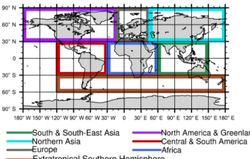
Figure 4.Total (summed over 10 years) model-simulated (JULES-WFDEI-GPCC, JULES-WFDEI-CRU and CARDAMOM),
observation-based (FLUXNET-MTE and MODIS) GPP fluxes for the 2001–2010 period on global and regional scales (tropics, subtropics and extratrop-ics) for three biome types (forest, grassland and shrub). Panel(a)shows the global total annual GPP,(b)for the tropics (30◦S–30◦N),(c)the extratropics (30–90◦N and 30–90◦S),(d)the tropics at 30◦S–15◦N and(e)the subtropics at 15–30◦N for forests, grasslands and shrubs.
The CV of the model-simulated and observation-based GPP fluxes range between 0.8 and 4 % for the mean monthly GPP, with the highest differences between the monthly val-ues being found for Northern Hemisphere winter and spring (February, March, April, November and December; Fig. 3b). This pattern is similar to the global average of the monthly climatologies (Fig. 3a).
The monthly anomalies (computed using the global mean values) expressed as percentages of the global mean of model-simulated monthly GPP (JULES-WFDEI-GPCC) compare equally well to both FLUXNET-MTE and MODIS GPP for 2001–2010, with both having root mean squared er-rors of 2.4 % and CARDAMOM having much lower year-to-year variation (Fig. 3c). JULES is able to capture simulated monthly anomalies from 2001 to 2010, with the exception of those in 2002 (Fig. 3c).
3.3 Global and regional comparison of simulated GPP for various biomes
In addition to examining the ability of JULES to simulate global GPP (integrated across all ecosystem types), the to-tal annual GPP for 2001–2010 was compared for various
biomes (forests, grasslands and shrubs) on global and re-gional scales (Fig. 4). This means that areas for model im-provement can be identified on scales smaller than the global. JULES overestimates GPP in all tropical land areas (central and South America, Africa, and South and South-East Asia), but is able to simulate it in the extratropics (Europe, northern Asia, North America and Greenland, and the extratropical Southern Hemisphere; Fig. 4).
When JULES was driven with WFDEI-GPCC (JULES-WFDEI-GPCC), JULES simulated average annual GPP to be 68, 62 and 9 PgC year−1 for forests, grasslands and shrubs, respectively (Fig. 4a). With the exception of shrubs, JULES overestimates average annual GPP by 30 % (24 %), 12 % (7 %) and 21 % (28 %) compared to MODIS, FLUXNET-MTE and CARDAMOM GPP, respectively, for forests (grasslands) compared to MODIS, FLUXNET-MTE and CARDAMOM GPP (Fig. 4a). Differences between JULES, MODIS, FLUXNET-MTE and CARDAMOM GPP for shrubs are small, with average annual GPP ranging within 9–10 PgC year−1(Fig. 4a).
40
N 30 E 0
� 20
a.. a.. CJ 10
0
60° S 30° S
--JULES-WFDEI-GPCC
---JULES-WFDEI-GPCC-1 degree ---JULES-PRINCETON --- CARDAMOM
---JULES-WFDEI-GPCC-2degree --MODIS
--FLUXNET-MTE
0 30° N 60° N 90° N
Figure 5. Zonal mean of total annual model-simulated (JULES-WFDEI-GPCC, JULES-WFDEI-GPCC-1degree, JULES-PRINCETON, CARDAMOM and JULES-WFDEI-GPCC-2degree) and observed (FLUXNET-MTE and MODIS) GPP fluxes for 2001–2010. JULES-WFDEI-GPCC, FLUXNET-MTE and MODIS are at 0.5◦×0.5◦spatial resolution.
and CARDAMOM estimates in the tropics (30◦S–30◦N; Fig. 4b) with a large negative bias in JULES occurring in the subtropics at 15–30◦N (Fig. 5). In the tropics, JULES simulates total annual GPP to be 55, 44 and 6 PgC year−1 for forests, grasslands and shrubs, respectively, for the 2001– 2010 period. JULES overestimates total annual GPP by 19–40 % compared to MODIS, FLUXNET-MTE and CAR-DAMOM GPP for forests and by 22–52 % for grasslands in the tropical regions (Fig. 4b). Differences between model-simulated and observation-based estimates of GPP are small in the tropics for shrubs, with total annual GPP ranging from 5 to 6 PgC year−1(Fig. 4b). In the extratropics (30–90◦N and 30–90◦S), differences between model and observed GPP are small, with average annual GPP for forests, grasslands and shrubs found to be 13–16, 18–23 and 3–5 PgC year−1, re-spectively (Fig. 4c).
Total annual GPP on the regional scale was further exam-ined by splitting the land area into seven regions (Fig. 1; Ta-ble 2). The tropical regions (30◦S–30◦N) were divided up into three regions: Central and South America, Africa, and South and South-East Asia. The extratropics (30–90◦N and 30–90◦S) were divided into four regions: Europe, northern Asia, North America and Greenland, and the extratropical Southern Hemisphere. JULES overestimates GPP in all three tropical land areas compared to MODIS, FLUXNET-MTE and CARDAMOM (Fig. 6c, e and f).
Differences in average annual GPP between JULES, MODIS, FLUXNET-MTE and CARDAMOM GPP range from 2.8 to 5.04, 3 to 6.1 and 0.8 to 3.7 PgC year−1 for
forests, grasslands and shrubs, respectively, in South and South-East Asia; 3.5–4.6, 3.2–4.2 and 0.1–4.2 PgC year−1 for forests, grasslands and shrubs, respectively, in Africa; and 1.9–5.6, 1.7–4.5 and 0.07–0.3 PgC year−1for forests, grass-lands and shrubs, respectively, in Central and South Amer-ica (Fig. 6c, e and f, respectively). In the extratropics, differ-ences between JULES, MODIS, FLUXNET-MTE and
CAR-DAMOM GPP are small, with average annual GPP ranging from 0.08 to 0.5, 0.1 to 1.5 and 0.029 to 0.12 PgC year−1
for forests, grasslands and shrubs, respectively, in Europe; 0.09–1.4, 0.7–1.8 and 0.2–0.6 PgC year−1for forests, grass-lands and shrubs, respectively, in northern Asia; 0.09– 0.14 PgC, 0.7–1.8 PgC year−1 and 0.03–0.2 PgC year−1 for forests, grasslands and shrubs, respectively, in the extrat-ropical Southern Hemisphere; and 0.005–5, 3–5 and 0.3– 0.5 PgC year−1 for forests, grasslands and shrubs, respec-tively, in North America and Greenland (Fig. 6a, b, d and g, respectively).
3.4 Sensitivity to spatial resolution
When simulating GPP on global and regional scales, there was little impact from varying spatial resolution (0.5◦×0.5◦, 1◦×1◦ and 2◦×2◦; Fig. 5). When simu-lations of GPP were performed at lower spatial resolu-tions (GPCC-1degree and JULES-WFDEI-GPCC-2degree; Table 1), the average annual global GPP at 0.5◦×0.5◦, 1◦×1◦and 2◦×2◦spatial resolutions was 140, 141 and 142 PgC year−1, respectively. The percentage differ-ences between JULES and the observation-based GPP esti-mates (MODIS and FLUXNET-MTE) at the various spatial resolutions are approximately equal with JULES differing from MODIS and FLUXNET-MTE by 8 and 25 %, respec-tively, at 0.5◦×0.5◦spatial resolution; by 8 and 26 %, respec-tively, at 1◦×1◦resolution; and by 9 and 26 %, respectively, at 2◦×2◦resolution.
The zonal mean of modelled total annual GPP at vari-ous spatial resolutions are approximately equal (Fig. 5). This insensitivity to spatial resolution is also found on regional scales (Fig. 6). This insensitivity to spatial resolution is a use-ful result since it means that model simulations can be per-formed at 2◦×2◦resolution with little difference to model output from the simulations at 0.5◦×0.5◦, and due to the lower computational cost, model run times (at 2◦×2◦ resolu-tion) are short (approximately 16×faster than the 0.5◦×0.5◦ resolution simulations).
3.5 Sensitivity to meteorological dataset
When JULES was driven with the PRINCETON dataset, simulated global GPP was found to be higher than that sim-ulated using WFDEI-GPCC by 3 PgC year−1 on average, with the largest differences occurring in the tropics (Figs. 5, 7a and 7d). When driven with the PRINCETON dataset (JULES-PRINCETON; Table 1), JULES simulates global GPP with an annual average of 144 PgC year−1for the 2001– 2010 period (Fig. 7d).
Figure 6. Total annual model-simulated (GPCC-1degree, JULES-PRINCETON, CARDAMOM and JULES-WFDEI-GPCC-2degree) and observed (FLUXNET-MTE and MODIS) GPP fluxes for the 2001–2010 period normalised by model-simulated (JULES-WFDEI-GPCC) GPP for various regions (Table 2) for three biome types (forest, grassland and shrub). Panels show normalised GPP(a)for Europe,(b)for northern Asia,(c)for South & South-Asia,(d)for extratropical Southern Hemisphere,(e)for Africa,(f)for Central & South America and(g)for North America & Greenland. The dotted line aty=1 represents where the model and observations match.
when driven with the WFDEI-GPCC dataset, which had an annual average global GPP of 140 PgC year−1. GPP simu-lated by JULES-WFDEI-GPCC was only higher than that of MODIS, FLUXNET-MTE (both at 0.5◦×0.5◦spatial reso-lution) and CARDAMOM (at 1◦×1◦resolution) by 8–25 %. The pattern in zonal mean of total annual GPP simulated by the model (when driven with PRINCETON) is similar to that when driven with WFDEI-GPCC (at 1◦×1◦spatial reso-lution), with differences between JULES-PRINCETON and JULES-WFDEI-GPCC-1degree and the observation-based estimates (MODIS and FLUXNET-MTE) being mostly in the tropics (Fig. 5).
Figure 7.Total annual model-simulated (JULES-WFDEI-GPCC-1degree and JULES-PRINCETON) GPP when simulations were performed with prescribed PFTs (vegetation competition switched off) and with different PFTs competing against each other (vegetation competition switched on) for 2001–2010. Panels(a)and(b)show the total annual JULES-WFDEI-GPCC-1degree GPP with vegetation competition switched off and on, respectively, and(c)shows the difference. Panels(d)and(e)show the total annual JULES-PRINCETON GPP with vegetation competition switched off and on, respectively, and(f)shows the difference. At the top right of(a),(b),(d)and(e), the average annual global GPP for 2001–2010 is displayed.
4 Discussion
4.1 How do estimates of total annual GPP compare to those from observational datasets? Can JULES capture the seasonal and interannual variability of GPP on global scales?
On global scales, JULES estimates the annual average GPP (combined GPP of all terrestrial ecosystems) to be 140 PgC year−1, which is greater than MODIS, FLUXNET-MTE and CARDAMOM GPP by 8–25 % (Fig. 2). The an-nual average MODIS, FLUXNET-MTE and CARDAMOM GPP estimates over 2001–2010 are 112, 130 and 114 PgC year−1, respectively (Fig. 2). Differences in these esti-mates are due to differences in forest and grassland GPP in the tropics (Fig. 4b). MODIS and CARDAMOM GPP esti-mates are similar on global and regional scales since both use MODIS LAI data to determine GPP (Fig. 2). In the extratropics, JULES was able to simulate GPP well com-pared to MODIS, FLUXNET-MTE and CARDAMOM since its phenology model and associated model parameters may have been designed for temperate regions. When JULES was driven with the WFDEI-GPCC dataset (at 0.5◦×0.5◦spatial resolution), the model was able to capture interannual vari-ability on the global scale (Fig. 3b).
The main difference between JULES and CARDAMOM GPP estimates was found in the tropics with CARDAMOM GPP being between the two observation-based datasets (Fig. 2e). Photosynthesis is also modelled differently in JULES and CARDAMOM. In JULES, leaf-level photosyn-thesis is calculated as the minimum of three limiting rates which is then scaled up to canopy level using the sum of the leaf-level fluxes in each canopy layer, scaled by leaf area (Clark et al., 2011). In CARDAMOM, GPP is
calcu-lated as a function of LAI, air temperature and radiation using the aggregated-canopy model (ACM; Williams et al., 1997). ACM is an emulator of the soil plant atmosphere (SPA) model and uses a set of equations to simulate daily GPP estimates produced by SPA (Williams et al., 1996).
JULES simulates lower GPP than MODIS, FLUXNET-MTE and CARDAMOM at 15–30◦N (Figs. 5 and 8). This large negative bias in JULES was due to the incorrect simula-tion of GPP in subtropical regions such as Mexico and south-ern China (Fig. 8a, b and c). The total annual MODIS and FLUXNET-MTE GPP estimates for 2001–2010 are higher than that simulated by JULES by 1 and 7 %, respectively, for Mexico, with CARDAMOM GPP estimates for the same period being lower than JULES GPP by 6 %. The tropical GPP fluxes for forests, grasslands and shrubs were further subdivided into two regions: (1) the tropics at 30◦S–15◦N (Fig. 4d) and (2) Mexico (Fig. 4e). The total (summed over 10 years) JULES GPP was similar for the two tropical re-gions at 30◦S–30◦N and 30◦S–15◦N, with positive biases in forest and grassland GPP (Fig. 4b and d). GPP in Mex-ico was similar for forests and grasslands, with differences in shrub GPP (Fig. 4e). The negative bias in JULES GPP in the subtropics is due to low LAI simulated by the model compared to MODIS (Fig. 5.10 in Slevin, 2016; Fig. 8d). MODIS LAI is used as input when generating the MODIS, FLUXNET-MTE and CARDAMOM GPP estimates.
Figure 8.Difference in total annual GPP between JULES-WFDEI-GPCC and the observation-based (FLUXNET-MTE and MODIS) and CARDAMOM estimates of GPP and in monthly mean LAI between JULES-WFDEI-GPCC and MODIS at latitudes 15–30◦N for the 2001–2010 period. Panel(a)shows the difference in GPP between FLUXNET-MTE and JULES,(b)between MODIS and JULES and(c)
between CARDAMOM and JULES. Panel(d)shows the difference in LAI between MODIS and JULES. A positive change in GPP means the observation-based estimates (FLUXNET-MTE and MODIS) or CARDAMOM estimate are higher than the model and in LAI means MODIS LAI is higher than JULES.
northwestern South America and southern China. The im-plementation of a drought-deciduous shrub PFT would help improve simulated GPP in these regions. In JULES, phe-nology is updated once per day by multiplying the annual maximum LAI by a scaling factor, which is calculated us-ing temperature-dependent leaf turnover rates. Leaf turnover rates are a function of surface air temperature and increase when the temperature drops below a certain value (this varies depending on the PFT). While this is suitable for deciduous broadleaf forests in temperate regions, such as northern Eu-rope, it will lead to inaccurate modelled LAI for drought-deciduous forests. Instead of modifying modelled LAI using a temperature-derived scaling factor, the scaling factor could be calculated by using periods of dryness as the controlling factor.
In general, when JULES was driven with the WFDEI-GPCC dataset on global scales (JULES-WFDEI-WFDEI-GPCC- (JULES-WFDEI-GPCC-1degree), it was found that simulated photosynthesis was Rubisco-limited (Figs. 5.6 and 5.7 in Slevin, 2016). Under saturated irradiance and limited atmospheric CO2
concentra-tions, the Rubisco-limiting rate is the main limiting factor (Marcus et al., 2008). Since the multi-layer approach for ra-diation interception and scaling from leaf-level to
canopy-level photosynthesis was used by JULES in this study, the model simulates competition between Rubisco-limited and light-limited photosynthesis for each canopy layer (Clark et al., 2011). This means that, lower in the canopy, there is in-creased light limitation, and in the upper layers of the canopy, Rubisco limitation dominates (Clark et al., 2011). Overall, the percentage of model grid boxes that were found to be Rubisco-limited was high (40–100 %), whereas the percent-age of model grid boxes that were found to be light-limited were small (0–20 %; Figs. 5.7 and 5.8, respectively, in Slevin, 2016). A description of the methods used to determine which limiting rate dominates each model grid box when calcu-lating potential leaf-level photosynthesis is provided in Ap-pendix F of Slevin (2016).
4.2 How do fluxes of GPP simulated by JULES compare for various biomes on the global and regional scales?
On global scales, JULES (JULES-WFDEI-GPCC) simu-lated average annual GPP to be 68, 62 and 9 PgC year−1 for forests, grasslands and shrubs, respectively. Simulated GPP for forests is higher than that calculated by Beer et al. (2010) (sum of the values for tropical, temperate and bo-real forests), with average annual GPP being 59 PgC year−1. Since Beer et al. (2010) provides average annual GPP values for tropical savannahs and grasslands, temperate grasslands and shrublands and croplands, these are summed in order to obtain average annual global GPP for grasslands and shrubs of 54.6 PgC year−1, which is lower than the JULES grass-lands and shrubs simulated total value of 71 PgC year−1.
Differences between MODIS and CARDAMOM esti-mates of average annual GPP are similar, with MODIS simulating average annual GPP to be 52.3, 50.1 and 9.4 PgC year−1 for forests, grasslands and shrubs, respec-tively, and CARDAMOM simulating average annual GPP to be 56.5, 48.6 and 9.2 PgC year−1 for forests, grass-lands and shrubs, respectively (Fig. 4a). The MODIS and CARDAMOM GPP estimates are similar due to MODIS LAI being assimilated into CARDAMOM GPP simulations. FLUXNET-MTE GPP is higher than the MODIS and CAR-DAMOM estimates for all biomes (Fig. 4). JULES simu-lates higher GPP than MODIS, FLUXNET-MTE and CAR-DAMOM on global scales and this was found to be due to higher GPP simulated by JULES for forests and grasslands in the tropics (Fig. 4b). The average annual GPP for shrubs was similar between model (JULES and CARDAMOM) and observation-based (MODIS and FLUXNET-MTE) estimates for all three regions (Fig. 4).
A simple sensitivity study of the model to changes in cli-mate (surface (2 m) air temperature, precipitation and atmo-spheric CO2concentrations) when simulating GPP on global
and regional scales for 2000–2010 was performed (Slevin, 2016). Only changes to one climate variable were made at a time due to complex interactions associated with multi-ple changes in climatic factors resulting in commulti-plex non-linear ecosystem responses which can be difficult to explain. JULES GPP was found to be sensitive to changes in all three climate variables, with modelled LAI only sensitive to changes in surface air temperature (Slevin, 2016). On the re-gional scale, for model simulations with varying air temper-ature, GPP increased with increasing temperature in the ex-tratropics, but decreased with increasing temperature in the tropics. Model simulations with varying precipitation on re-gional scales show the same trend as those on global scales, with GPP increasing with increasing precipitation and de-creasing with dede-creasing precipitation except for the magni-tude of the effect observed. More detailed information on the sensitivity study is provided in chap. 6 of the PhD thesis of Darren Slevin (Slevin, 2016).
There are two possible reasons for the larger simulated GPP in the tropics at 30◦S–15◦N. Firstly, the high bias in the tropics during December, January, February and March (Figs. 2e and 3b) implies that JULES GPP is overestimated in the tropical wet season. The lower air temperatures and higher soil moisture availability during the wet season as a re-sult of the meteorological data leads to higher simulated GPP in these regions. Secondly, the higher tropical GPP is due to the incorrect simulation of GPP by the PFTs in the version of JULES (version 3.4.1) used in this study. In this version, the PFT used to represent tropical forests is the broadleaf tree, which is used to simulate GPP in both tropical and temperate regions. This means that the model parameters used for the broadleaf tree PFT may not be suitable for simulating GPP in the tropics. The addition of extra PFTs more suited to tropi-cal regions (such as tropitropi-cal broadleaf evergreen (in version 4.2) and a drought-deciduous PFT) and a phenology model which can simulate LAI in tropical regions would both im-prove GPP simulations.
By dividing the global land area into seven regions (Ta-ble 2), it was found that for all three tropical regions (cen-tral and South America, Africa, and South and South-East Asia), JULES overestimated total annual GPP for forests, grasslands and shrubs (Fig. 6c, e, and f). In the four extra-tropical regions (Europe, northern Asia, extraextra-tropical South-ern Hemisphere and North America and Greenland), JULES simulated similar GPP to MODIS, FLUXNET-MTE and CARDAMOM for the three biomes in Europe and the tratropical Southern Hemisphere (Fig. 6a and d), with the ex-ception of northern Asia, and North America and Greenland, where the model is either equal to or lower than all three datasets (Fig. 6b and g).
One possibility for the higher GPP estimates in northern Asia and North America and Greenland is due to a different land cover map being used by the observation-based datasets (MODIS and FLUXNET-MTE) and JULES. The PFT frac-tions specified in the land cover map used by JULES were used to calculate the GPP estimates for the forests, grasslands and shrubs biomes for MODIS, FLUXNET-MTE and CAR-DAMOM. So for a particular grid box, the land cover map of JULES may specify a shrub, but in the land cover map used by MODIS or FLUXNET-MTE, it may be a needle-leaf tree. Another possibility is that shrubs in these northern regions have adapted to the cold environment and the lower surface air temperatures have a lesser impact on photosynthe-sis than they do on shrubs in warmer climates. The addition of a shrub PFT to JULES which is adapted to cold climates may improve GPP estimates in these regions.
4.3 How sensitive are fluxes of GPP to the spatial resolution of the model?
respec-tively. This pattern was also observed in the zonal mean of total annual GPP (Fig. 5). The insensitivity of the model to spatial resolution on the global scale was also observed on the regional scale when comparing simulated GPP fluxes for forests, grasslands and shrubs in the tropics and extratropics (Fig. 6).
Little research has been performed on the effects of spatial resolution on JULES simulations (as well as those of other LSMs). Studies using atmospheric chemistry models have shown that the spatial resolution of the input meteorologi-cal data can affect model output (Ito et al., 2009; Pugh et al., 2013; Schaap et al., 2015). The results found here agree with those from Compton and Best (2011). Compton and Best (2011) showed that JULES was insensitive to spatial resolu-tion when the WFD dataset was regridded from half-degree to 1-degree and 2-degree when simulating the terrestrial hy-drological cycle. It was found that spatial resolution had little or no effect on simulations of global mean total evaporation and total runoff. However, the study showed that JULES was sensitive to temporal resolution when simulating the same hydrological components.
Using a different soil ancillary dataset or land cover map (which specifies the PFT fractions) may have a larger im-pact than changing the spatial resolution. The regridding method used in this study was the conservative method, which preserves the same information when interpolating from 0.5◦×0.5◦to 1◦×1◦and 2◦×2◦ spatial resolutions, and results in only small differences in global GPP between the model simulations with varying spatial resolution. These small differences are due to differences in the PFT fractions of the land cover map after regridding.
4.4 Is the meteorological dataset used to drive the model important on the global scale?
When JULES was driven with the PRINCETON dataset at 1◦×1◦ spatial resolution (Table 2), the annual average global GPP was slightly higher, by 3 PgC year−1, than that simulated by JULES when driven with the WFDEI-GPCC dataset at the same resolution. In general, differences in GPP fluxes for model simulations driven using WFDEI-GPCC and PRINCETON are mainly in the deep tropics (at 5◦N–5◦S), with JULES-WFDEI-GPCC-1degree simulating higher GPP than JULES-PRINCETON, and in the extrat-ropics at 30–60◦N, JULES-PRINCETON simulates slightly higher GPP (Figs. 5 and 6).
The higher simulated GPP at 5◦N–5◦S in the Amazo-nian, African and South-East Asian tropics in the WFDEI-GPCC-driven simulation is due to lower surface air temper-atures (Fig. G.6a and c in Slevin, 2016) and higher precip-itation (Fig. G.6b and d in Slevin, 2016) in these regions (Slevin, 2016). In extratropical regions, such as northern Eurasia (above 60◦N), there are differences in the meteo-rological datasets with slightly higher downward shortwave radiation fluxes and surface air temperatures in the
PRINCE-TON dataset, with little difference between the JULES sim-ulations driven with either WFDEI-GPCC or PRINCETON in this region (Fig. 5).
Other studies have shown that the meteorological dataset used to drive LSMs is a large source of uncertainty in global land surface modelling (Hicke, 2005; Jung et al., 2007; Poul-ter et al., 2011). Different methods are used to create time series of global gridded climate data in order to drive LSMs, and this can introduce uncertainty that can propagate through model simulations (Zhao et al., 2006). Even on the point scale, differences in simulated GPP were observed when driving JULES with the WFDEI-GPCC and PRINCETON datasets (Slevin et al., 2015). As in this study, it also occurred in the tropics.
When JULES was driven with the PRINCETON dataset, simulated photosynthesis was mostly Rubisco-limited (Figs. 5.25 and 5.6 in Slevin, 2016). This is a similar result to when JULES was driven with the WFDEI-GPCC dataset. When model grid-box fractions were compared be-tween the WFDEI-GPCC- and PRINCETON-driven model simulations, photosynthesis in the PRINCETON-driven sim-ulation was more Rubisco-limited than that when driven with WFDEI-GPCC (Fig. 5.26 in Slevin, 2016); this is due to higher surface air temperatures (used in calculating photo-synthesis for the Rubisco limiting rate) in the PRINCETON dataset (Fig. G.6a and c in Slevin, 2016).
Since the WFDEI-GPCC dataset has lower downward shortwave radiation than PRINCETON, photosynthesis in the WFDEI-GPCC-driven simulation was more light-limited than the PRINCETON simulation (Figs. 5.27, G.5a and G.5c in Slevin, 2016). The number of model grid boxes in which transport limitation dominated in the PRINCETON-driven simulation were fewer than those for the JULES-WFDEI-GPCC-1degree model simulation (Fig. 5.28 in Slevin, 2016). There is a pronounced geographical varia-tion with the WFDEI-GPCC-driven simulavaria-tion being more transport-limited in the tropics and the PRINCETON-driven simulation being more transport-limited in the extratropics (Fig. 5.28 in Slevin, 2016). This is likely due to the lower surface air temperatures in the WFDEI-GPCC, which results in lower potential leaf-level photosynthesis for C3 and C4 plants in the extratropics and tropics, respectively.
stretches from the Atlantic Ocean in the west to the Ethiopian Highlands in the east of Africa) and northern Australia, there is higher GPP with prescribed PFTs (Fig. 7c and f). These are also fire-prone regions. The version of JULES used in this study has no fire or deforestation module implemented, and TRIFFID may overestimate woody cover and therefore GPP.
In terms of global GPP, the WFDEI-GPCC- and PRINCETON-driven simulations produce similar increases (Fig. 7b and e). However, the spatial pattern is slightly dif-ferent, with higher GPP simulated in the Amazon region when JULES was driven with the WFDEI-GPCC dataset and higher GPP in southern Brazil and Argentina and Southeast Asia when JULES was driven with the PRINCETON dataset (Fig. 7c and f). The spatial pattern of simulated GPP is more sensitive to the meteorological data than the annual average global GPP if competition between PFTs is allowed. This may be due to compensating differences in the sensitivity of the model to the two meteorological datasets.
5 Conclusions
An evaluation of JULES was performed on global and re-gional scales with simulated GPP compared to global grid-ded (0.5◦×0.5◦ spatial and monthly temporal resolution) estimates of GPP derived from upscaled FLUXNET obser-vations (FLUXNET-MTE), satellite obserobser-vations (MODIS) and that produced by the CARDAMOM data assimilation framework (CARDAMOM). JULES simulated higher aver-age annual global GPP than FLUXNET-MTE, MODIS and CARDAMOM, but on regional scales, differences arose in the tropics. It was found that JULES was able to capture in-terannual variability on the global scale.
Differences in GPP between JULES and the benchmark-ing datasets (FLUXNET-MTE, MODIS and CARDAMOM) at 15–30◦N is due to higher FLUXNET-MTE, MODIS and CARDAMOM GPP in regions such as Mexico and southern China. These differences may be due to a lack of drought-deciduous PFTs in JULES. The inclusion of these PFTs could improve GPP simulations at latitude 15–30◦N. By di-viding the global land area into seven regions, it was found that all three tropical regions (Central and South Amer-ica, AfrAmer-ica, and South and South-East Asia) contribute to model–observation differences on the global scale compared to FLUXNET-MTE and MODIS. The model can reasonably reproduce GPP estimates in the four extratropical regions (Europe, northern Asia, North America and Greenland, and the extratropical Southern Hemisphere).
Improved GPP simulations in the tropics could be at-tained with the introduction of more PFT classes and their associated model parameters. In the version of JULES used in this study (3.4.1), each model grid box is composed of nine different surface types and five of these are PFTs. Since model version 4.2, each JULES grid box contains nine
PFTS (tropical broadleaf evergreen, temperate broadleaf ev-ergreen, broadleaf deciduous, needleleaf evev-ergreen, needle-leaf deciduous, C3, C4, evergreen shrub, deciduous shrub; Harper et al., 2016). In addition to these PFTs, a phenology model which can simulate LAI in both temperate and tropi-cal regions would help to reduce differences between model-simulated and observation-based estimates of GPP in the dry and wet tropics.
When JULES was driven on the global and regional scale with the WFDEI-GPCC dataset at various spatial resolutions (0.5◦×0.5◦, 1◦×1◦and 2◦×2◦), it was found that the model was insensitive to spatial resolution. Similar results were shown by Compton and Best (2011) when simulating com-ponents of the terrestrial hydrological cycle. Differences be-tween high (0.5◦×0.5◦) and low (2◦×2◦) spatial resolution simulations of GPP are very similar. This means that low-spatial-resolution model simulations on these scales can be performed in place of high resolution when simulating GPP and results in shorter model run times.
The meteorological dataset used to drive LSMs on the global scale is an important source of model uncertainty (Poulter et al., 2011). By using a different meteorological dataset (PRINCETON) to drive the model, it was found that simulated GPP was similar to that when the model was driven with the WFDEI-GPCC dataset (at 1◦×1◦ spatial resolu-tion), with exceptions to this being in the tropics and the northern extratropics. Differences in the tropics are due to lower surface air temperatures and higher precipitation (and therefore increased soil moisture availability) in the WFDEI-GPCC dataset and in the extratropics, due to higher air tem-peratures in the PRINCETON dataset. Photosynthesis in the WFDEI-GPCC- and PRINCETON-driven simulations were Rubisco-limited. The model simulations in this study were largely performed with prescribed PFTs (i.e. no competi-tion between PFTs was allowed). With competicompeti-tion between PFTs, the annual average global GPP was higher by 15 and 17 %, for the WFDEI-GPCC- and PRINCETON-driven sim-ulations, respectively, with the spatial pattern of simulated GPP more sensitive to the meteorological data used.
representing temperate, boreal, wet and dry tropical ecosys-tems. Overall, there is not much difference in retrieved pa-rameters because of the large error and/or uncertainty terms used when computing the likelihood.
In general, differences between JULES GPP and the benchmarking datasets (FLUXNET-MTE, MODIS and CARDAMOM) occur mostly in the tropics, with differences at 15–30◦N possibly due to a lack of drought-deciduous PFTs in JULES. When JULES was driven with different me-teorological datasets (WFDEI-GPCC and PRINCETON), the WFDEI-GPCC-driven model simulations estimated higher GPP in the tropics (at 5◦N–5◦S) and the PRINCETON-driven model simulations higher GPP in the extratropics (at 30–60◦N). The meteorological dataset used to drive JULES was found to be a source of model uncertainty in the trop-ics, though this may be due to model error. By using a dif-ferent precipitation product (WFDEI-CRU), differences in JULES GPP were very small. Finally, when model simula-tions of GPP were performed at various spatial resolusimula-tions (0.5◦×0.5◦, 1◦×1◦and 2◦×2◦), JULES was found to be insensitive to spatial resolution.
Code and data availability. The JULES model code (v3.4.1) is stored at the Met Office Science Repository Service in the JULES repository (https://code.metoffice.gov.uk/trac/jules), and access to the code can be requested from the official website of JULES (http: //jules.jchmr.org/). The outputs from the JULES model simulations reported in this paper have been deposited online at DataShare, the University of Edinburgh’s digital repository of multidisciplinary re-search datasets, https://doi.org/10.7488/ds/1461. The ancillary data (soil, vegetation, etc.) used for these simulations have also been de-posited on DataShare (https://doi.org/10.7488/ds/1995).
Author contributions. DS, SFBT and MW designed the research. DS, J-FE and AAB performed the model simulations. DS, SFBT and MW analysed the data. DS prepared the paper with contribu-tions from all co-authors.
Competing interests. The authors declare that they have no conflict of interest.
Acknowledgements. The authors would like to thank the anony-mous reviewers and editor for their valuable comments which improved the quality of the paper. We would like to gratefully acknowledge the School of GeoSciences, University of Edinburgh, which provided Darren Slevin with a School Scholarship that allowed him to pursue his PhD research, during which this work was carried out. Part of this work was conducted at the Jet Propulsion Laboratory, California Institute of Technology, under a contract with NASA and supported by the Natural Environment Research Council (NERC) and the UK National Centre for Earth Observation (NCEO). This work would not have been possible without help from the following people. Rich Ellis at the Centre for
Ecology and Hydrology (CEH) provided the soil and vegetation ancillary files as well as advice on modifying the namelist files in order to set up the model simulations to run on a 2-D grid. Doug Clark (also at CEH) provided advice on model spin-up on global scales. Information on the snow schemes used by JULES and advice on which one to use on global scales were provided by Richard Essery. Graham Weedon provided invaluable advice on using the WFDEI meteorological dataset.
Edited by: Hisashi Sato
Reviewed by: two anonymous referees
References
Anav, A., Friedlingstein, P., Beer, C., Ciais, P., Harper, A., Jones, C., Murray-Tortarolo, G., Papale, D., Parazoo, N. C., Peylin, P., Piao, S., Sitch, S., Viovy, N., Wiltshire, A., and Zhao, M.: Spatio-temporal patterns of terrestrial gross pri-mary production: A review, Rev. Geophys., 53, 785–818, https://doi.org/10.1002/2015RG000483, 2015.
Battin, T. J., Luyssaert, S., Kaplan, L. A., Aufdenkampe, A. K., Richter, A., and Tranvik, L. J.: The boundless carbon cycle, Nat. Geosci., 2, 598–600, https://doi.org/10.1038/ngeo618, 2009. Beer, C., Reichstein, M., Tomelleri, E., Ciais, P., Jung, M.,
Carval-hais, N., Rödenbeck, C., Arain, M. A., Baldocchi, D., Bonan, G. B., Bondeau, A., Cescatti, A., Lasslop, G., Lindroth, A., Lo-mas, M., Luyssaert, S., Margolis, H., Oleson, K. W., Roupsard, O., Veenendaal, E., Viovy, N., Williams, C., Woodward, F. I., and Papale, D.: Terrestrial Gross Carbon Dioxide Uptake: Global Distribution and Covariation with Climate, Science, 329, 834– 838, https://doi.org/10.1126/science.1184984, 2010.
Best, M. J., Pryor, M., Clark, D. B., Rooney, G. G., Essery, R. L. H., Ménard, C. B., Edwards, J. M., Hendry, M. A., Porson, A., Gedney, N., Mercado, L. M., Sitch, S., Blyth, E., Boucher, O., Cox, P. M., Grimmond, C. S. B., and Harding, R. J.: The Joint UK Land Environment Simulator (JULES), model description – Part 1: Energy and water fluxes, Geosci. Model Dev., 4, 677–699, https://doi.org/10.5194/gmd-4-677-2011, 2011.
Bloom, A. A. and Williams, M.: Constraining ecosystem carbon dy-namics in a data-limited world: integrating ecological “common sense” in a model–data fusion framework, Biogeosciences, 12, 1299–1315, https://doi.org/10.5194/bg-12-1299-2015, 2015. Bloom, A. A., Exbrayat, J.-F., van der Velde, I. R., Feng, L.,
and Williams, M.: The decadal state of the terrestrial carbon cycle: Global retrievals of terrestrial carbon allocation, pools, and residence times, P. Natl. Acad. Sci. USA, 113, 1285–1290, https://doi.org/10.1073/pnas.1515160113, 2016.
Blyth, E., Gash, J., Lloyd, A., Pryor, M., Weedon, G. P., and Shut-tleworth, J.: Evaluating the JULES Land Surface Model Energy Fluxes Using FLUXNET Data, J. Hydrometeorol., 11, 509–519, https://doi.org/10.1175/2009JHM1183.1, 2010.
Bonan, G. B.: Forests and Climate Change: Forcings, Feedbacks, and the Climate Benefits of Forests, Science, 320, 1444–1449, https://doi.org/10.1126/science.1155121, 2008.
Bonan, G. B., Lawrence, P. J., Oleson, K. W., Levis, S., Jung, M., Reichstein, M., Lawrence, D. M., and Swenson, S. C.: Improving canopy processes in the Community Land Model version 4 (CLM4) using global flux fields empirically in-ferred from FLUXNET data, J. Geophys. Res., 116, G02014, https://doi.org/10.1029/2010JG001593, 2011.
Burke, E. J., Dankers, R., Jones, C. D., and Wiltshire, A. J.: A retrospective analysis of pan Arctic permafrost using the JULES land surface model, Clim. Dynam., 41, 1025–1038, https://doi.org/10.1007/s00382-012-1648-x, 2013.
Canadell, J. G., Le Quéré, C., Raupach, M. R., Field, C. B., Buiten-huis, E. T., Ciais, P., Conway, T. J., Gillett, N. P., Houghton, R. A., and Marland, G.: Contributions to accelerating atmo-spheric CO2 growth from economic activity, carbon intensity,
and efficiency of natural sinks, P. Natl. Acad. Sci. USA, 104, 18866–18870, https://doi.org/10.1073/pnas.0702737104, 2007. Chadburn, S., Burke, E., Essery, R., Boike, J., Langer, M.,
Heikenfeld, M., Cox, P., and Friedlingstein, P.: An im-proved representation of physical permafrost dynamics in the JULES land-surface model, Geosci. Model Dev., 8, 1493–1508, https://doi.org/10.5194/gmd-8-1493-2015, 2015.
Chapin III, F. S., Matson, P. A., and Vitousek, P.: Principles of Terrestrial Ecosystem Ecology, Springer-Verlag New York, https://doi.org/10.1007/978-1-4419-9504-9, 2012.
Clark, D. B., Mercado, L. M., Sitch, S., Jones, C. D., Gedney, N., Best, M. J., Pryor, M., Rooney, G. G., Essery, R. L. H., Blyth, E., Boucher, O., Harding, R. J., Huntingford, C., and Cox, P. M.: The Joint UK Land Environment Simulator (JULES), model description – Part 2: Carbon fluxes and vegetation dynamics, Geosci. Model Dev., 4, 701–722, https://doi.org/10.5194/gmd-4-701-2011, 2011.
Compton, E. and Best, M.: Impact of spatial and temporal reso-lution on modelled terrestrial hydrological cycle components, Tech. Rep. 44, WATCH Technical Report, 19 pp., available at: http://www.eu-watch.org (last access: 7 July 2017), 2011. Cox, P. and Jones, C.: Illuminating the Modern Dance
of Climate and CO2, Science, 321, 1642–1644,
https://doi.org/10.1126/science.1158907, 2008.
Cox, P. M.: Description of the “TRIFFID” Dynamic Global Vege-tation Model, Tech. Rep. 24, Hadley Centre, Met Office, London Road, Bracknell, Berkshire, RG12 2SY, UK, 2001.
Cox, P. M., Huntingford, C., and Harding, R. J.: A canopy conductance and photosynthesis model for use in a GCM land surface scheme, J. Hydrol., 212–213, 79–94, https://doi.org/10.1016/S0022-1694(98)00203-0, 1998. Cox, P. M., Betts, R. A., Bunton, C. B., Essery, R. L. H.,
Rown-tree, P. R., and Smith, J.: The impact of new land surface physics on the GCM simulation of climate and climate sensitivity, Clim. Dynam., 15, 183–203, https://doi.org/10.1007/s003820050276, 1999.
Dalmonech, D., Zaehle, S., Schürmann, G. J., Brovkin, V., Reick, C., and Schnur, R.: Separation of the Effects of Land and Climate Model Errors on Simulated Contemporary Land Carbon Cycle Trends in the MPI Earth System Model version 1, J. Climate, 28, 272–291, https://doi.org/10.1175/JCLI-D-13-00593.1, 2014.
Deardorff, J. W.: Efficient Prediction of Ground Sur-face Temperature and Moisture, With Inclusion of a Layer of Vegetation, J. Geophys. Res., 83, 1889–1903, https://doi.org/10.1029/JC083iC04p01889, 1978.
Foley, J. A., Prentice, I. C., Ramankutty, N., Levis, S., Pol-lard, D., Sitch, S., and Haxeltine, A.: An integrated biosphere model of land surface processes, terrestrial carbon balance, and vegetation dynamics, Global Biogeochem. Cy., 10, 603–628, https://doi.org/10.1029/96GB02692, 1996.
Friedlingstein, P., Cox, P., Betts, R., Bopp, L., Von Bloh, W., Brovkin, V., Cadule, P., Doney, S., Eby, M., Fung, I., Bala, G., John, J., Jones, C., Joos, F., Kato, T., Kawamiya, M., Knorr,W., Lindsay, K., Matthews, H. D., Raddatz, T., Rayner, P., Reick, C., Roeckner, E., Schnitzler, K.-G., Schnur, R., Strassmann, K., Weaver, A. J., Yoshikawa, C., and Zeng, N.: Climate-Carbon Cycle Feedback Analysis: Results from the C4MIP Model Intercomparison, J. Climate, 19, 3337–3353, https://doi.org/10.1175/JCLI3800.1, 2006.
Friedlingstein, P., Meinshausen, M., Arora, V. K., Jones, C. D., Anav, A., Liddicoat, S. K., and Knutti, R.: Uncertainties in CMIP5 climate projections due to carbon cycle feedbacks, J. Cli-mate, 27, 511–526, https://doi.org/10.1175/JCLI-D-12-00579.1, 2014.
Galbraith, D., Levy, P. E., Sitch, S., Huntingford, C., Cox, P., Williams, M., and Meir, P.: Multiple mechanisms of Ama-zonian forest biomass losses in three dynamic global vegeta-tion models under climate change, New Phytol., 187, 647–665, https://doi.org/10.1111/j.1469-8137.2010.03350.x, 2010. Giglio, L., Randerson, J. T., and van der Werf, G. R.:
Analy-sis of daily, monthly, and annual burned area using the fourth-generation global fire emissions database (GFED4), J. Geophys. Res.-Biogeo., 118, 317–328, https://doi.org/10.1002/jgrg.20042, 2013.
Harper, A. B., Cox, P. M., Friedlingstein, P., Wiltshire, A. J., Jones, C. D., Sitch, S., Mercado, L. M., Groenendijk, M., Robertson, E., Kattge, J., Bönisch, G., Atkin, O. K., Bahn, M., Cornelis-sen, J., Niinemets, Ü., Onipchenko, V., Peñuelas, J., Poorter, L., Reich, P. B., Soudzilovskaia, N. A., and Bodegom, P. V.: Im-proved representation of plant functional types and physiology in the Joint UK Land Environment Simulator (JULES v4.2) us-ing plant trait information, Geosci. Model Dev., 9, 2415–2440, https://doi.org/10.5194/gmd-9-2415-2016, 2016.
Hicke, J. A.: NCEP and GISS solar radiation data sets available for ecosystem modeling: Description, differences, and impacts on net primary production, Global Biogeochem. Cy., 19, GB2006, https://doi.org/10.1029/2004GB002391, 2005.
Hiederer, R. and Köchy, M.: Global Soil Organic Carbon Esti-mates and the Harmonized World Soil Database, Tech. Rep. EUR 25225 EN, Publications Office of the European Union, Luxem-bourg, 2011.