www.geosci-model-dev.net/10/1233/2017/ doi:10.5194/gmd-10-1233-2017
© Author(s) 2017. CC Attribution 3.0 License.
Modeling surface water dynamics in the Amazon Basin using
MOSART-Inundation v1.0: impacts of geomorphological
parameters and river flow representation
Xiangyu Luo1, Hong-Yi Li1,2, L. Ruby Leung1, Teklu K. Tesfa1, Augusto Getirana3, Fabrice Papa4,5, and Laura L. Hess6
1Pacific Northwest National Laboratory, Richland, WA 99352, USA 2Montana State University, Bozeman, MT 59715, USA
3NASA Goddard Space Flight Center, Greenbelt, MD 20771, USA
4LEGOS/IRD, Universite de Toulouse, IRD-CNRS-CNES-UPS, Toulouse 31400, France
5Indo-French Cell for Water Sciences, IISc-NIO-IITM–IRD Joint International Laboratory, IISc, Bangalore, India 6University of California, Santa Barbara, CA 93106, USA
Correspondence to:L. Ruby Leung ([email protected])
Received: 6 August 2016 – Discussion started: 10 August 2016
Revised: 18 February 2017 – Accepted: 20 February 2017 – Published: 23 March 2017
Abstract. In the Amazon Basin, floodplain inundation is a key component of surface water dynamics and plays an important role in water, energy and carbon cycles. The Model for Scale Adaptive River Transport (MOSART) was extended with a macroscale inundation scheme for repre-senting floodplain inundation. The extended model, named MOSART-Inundation, was used to simulate surface hydrol-ogy of the entire Amazon Basin. Previous hydrologic mod-eling studies in the Amazon Basin identified and addressed a few challenges in simulating surface hydrology of this basin, including uncertainties of floodplain topography and chan-nel geometry, and the representation of river flow in reaches with mild slopes. This study further addressed four aspects of these challenges. First, the spatial variability of vegetation-caused biases embedded in the HydroSHEDS digital eleva-tion model (DEM) data was explicitly addressed. A vegeta-tion height map of about 1 km resoluvegeta-tion and a land cover dataset of about 90 m resolution were used in a DEM correc-tion procedure that resulted in an average elevacorrec-tion reduccorrec-tion of 13.2 m for the entire basin and led to evident changes in the floodplain topography. Second, basin-wide empirical for-mulae for channel cross-sectional dimensions were refined for various subregions to improve the representation of spa-tial variability in channel geometry. Third, the channel Man-ning roughness coefficient was allowed to vary with the
chan-nel depth, as the effect of riverbed resistance on river flow generally declines with increasing river size. Lastly, backwa-ter effects were accounted for to betbackwa-ter represent river flow in mild-slope reaches. The model was evaluated against in situ streamflow records and remotely sensed Envisat altime-try data and Global Inundation Extent from Multi-Satellites (GIEMS) inundation data. In a sensitivity study, seven sim-ulations were compared to evaluate the impacts of the five modeling aspects addressed in this study. The comparisons showed that representing floodplain inundation could signif-icantly improve the simulated streamflow and river stages. Refining floodplain topography, channel geometry and Man-ning roughness coefficients, as well as accounting for back-water effects had notable impacts on the simulated surface water dynamics in the Amazon Basin. The understanding ob-tained in this study could be helpful in improving modeling of surface hydrology in basins with evident inundation, espe-cially at regional to continental scales.
1 Introduction
land surface and the atmosphere. For instance, surface wa-ter bodies are important natural sources of greenhouse gases (e.g., carbon dioxide and methane) (Bousquet et al., 2006; Richey et al., 2002). Extreme events such as river inunda-tion have extraordinary effects on land surface–groundwater interactions and sediment and nutrient exchanges between rivers and floodplains, and thereby influence land and aquatic ecosystems as well as their feedback to the atmosphere. Therefore, improving parameterizations of surface water dy-namics is meaningful in studying the land–climate linkage.
Many previous studies of surface-hydrology modeling were conducted for the Amazon River, which is the largest river of the globe and accounts for about 18 % of the total continental freshwater discharge to oceans (Dai and Tren-berth, 2002). Seasonal floods occur every year and wetlands occupy a considerable fraction of the total area in the basin (Hess et al., 2003, 2015a). River and inundation dynamics were simulated by using 2-D hydrodynamic models in the central Amazon Basin (e.g., Baugh et al., 2013; Wilson et al., 2007). Using fine-resolution grid cells (e.g., ∼300 m) as computation units, 2-D hydrodynamic models could repre-sent water flow over floodplains. They were not applied at regional or larger scales due to computational cost. On the other hand, some computationally efficient macroscale in-undation schemes were used in a few continental-scale hy-drologic models for the entire Amazon Basin (Coe et al., 2008; Decharme et al., 2008; Getirana et al., 2012; Paiva et al., 2013a; Vörösmarty et al., 1989; Yamazaki et al., 2011), which could capture some aspects of surface water dynam-ics fairly well. These previous studies also identified and ad-dressed a number of modeling challenges, including uncer-tainties in model inputs of floodplain and channel morphol-ogy, flow parameterization for gentle-gradient reaches, etc.
The Model for Scale Adaptive River Transport (MOSART) was developed to simulate terrestrial sur-face water flow from hillslopes to the basin outlet (Li et al., 2013). It was designed to be applicable at the local, regional or continental scale. Some details of this model are provided in Sect. 2.1. In this study, the MOSART model was extended with a macroscale inundation scheme for repre-senting floodplain inundation. The extended model, named MOSART-Inundation, was applied to the entire Amazon Basin. In addition, some efforts were made to further address four aspects of the aforementioned challenges: (1) while alleviating the vegetation-caused biases embedded in the digital elevation model (DEM) data, we explicitly considered the spatial variability of those biases; (2) the approach for estimating channel cross-sectional dimensions was refined to improve its representation of the spatial variability in channel geometry; (3) the Manning roughness coefficient of the channel was allowed to vary with the channel depth; and (4) backwater effects were accounted for to better represent river flow in gentle-gradient reaches.
Topography data are essential inputs in hydrologic mod-eling. At present, the common practice is to use the DEM to
represent topography. Because the coverage of high-accuracy DEM data (e.g., with elevation errors less than 1 m) is lim-ited, hydrologic modeling at regional or larger scales uses DEM data obtained by spaceborne sensors. The Shuttle Radar Topography Mission (SRTM) DEM data have been widely used for hydrologic modeling, but some factors limit their accuracy. In forested regions such as the Amazon Basin, primary biases in the SRTM DEM data were caused by veg-etation cover because the radar signal was not able to pene-trate the vegetation canopy (Sanders, 2007). Previous studies in the Amazon Basin adopted various approaches to alleviate the vegetation-caused biases embedded in the SRTM data. In some modeling studies, elevation values were lowered by a constant in forested areas of the entire basin, so the spa-tial variability of vegetation heights was ignored (Coe et al., 2008; Paiva et al., 2013a). In a few hydrodynamic modeling studies for the central Amazon Basin, the vegetation-caused biases in the SRTM elevations were derived from spatially varying vegetation heights. For example, Wilson et al. (2007) estimated the vegetation height distribution based on their surveyed heights of various vegetation types, and a map of vegetation types by Hess et al. (2003) and Baugh et al. (2013) utilized a global dataset of spatially distributed vegetation heights developed by Simard et al. (2011). These two studies estimated the vegetation-caused biases as products of spa-tially varying vegetation heights and a fixed percentage. In this study, we used the HydroSHEDS DEM data which were derived from the SRTM data and inherited the vegetation-caused biases. To alleviate those biases, we used a method similar to that of Baugh et al. (2013). Besides the vegeta-tion height map by Simard et al. (2011), we also used a land cover dataset for wetlands of the lowland Amazon Basin de-veloped by Hess et al. (2003, 2015a). A “bare-earth” DEM of the Amazon Basin was created and employed in the hydro-logic modeling for the entire basin. To our knowledge, this was the first time that the spatial variability of vegetation-caused biases in the DEM data was explicitly considered in hydrologic modeling for the entire Amazon Basin.
were estimated by using one set of channel geometry for-mulae and corresponding parameters which represent the av-erage characteristics of the entire basin. Thus, for different subregions of the basin, channel cross-sectional dimensions derived from the same formulae and parameters contained biases of various magnitudes. Hydrologic modeling results were demonstrated to be sensitive to channel cross-sectional dimensions and shapes (Getirana et al., 2013; Neal et al., 2015; Paiva et al., 2013a; Yamazaki et al., 2011), so improv-ing the representation of channel morphology could be im-portant. In this study, the basin-wide parameters for the chan-nel geometry formulae were refined for various subregions of the Amazon Basin based on local channel morphology infor-mation to better represent the spatial variability in channel morphology.
The Manning formula has been used for estimating flow velocities of rivers in many continental-scale hydrologic models. In this formula, the Manning roughness coefficient (also abbreviated to Manning coefficient hereinafter; in this article, the Manning roughness coefficient discussed is for river channels) is a key and sensitive parameter (Paiva et al., 2013a; Yamazaki et al., 2011) that can only be esti-mated empirically. In previous studies of the Amazon Basin, the Manning coefficient was determined using various ap-proaches: (a) a constant value for the entire basin (Beighley et al., 2009; Yamazaki et al., 2011); (b) different values for different subregions as a result of calibration using hydro-graphs of major rivers (Paiva et al., 2013a); and (c) diverse values dependent on the channel cross-sectional dimensions that vary spatially (Getirana et al., 2012, 2013). For natural river channels, the Manning coefficient depends on many fac-tors, including riverbed roughness, cross-sectional geometry and channel sinuosity (Arcement and Schneider, 1989). The significant variations of these factors within a basin under-mine the rationale of using a uniform Manning coefficient across the entire basin or using a few Manning coefficients for different subregions of the basin. The approaches of the aforementioned category (c) reflect the general phenomenon that the relative importance of riverbed friction in river flow becomes smaller for larger rivers, and can be used to repre-sent the dominant spatial variability of the Manning coeffi-cients. We adopted a method of category (c), similar to those of Decharme et al. (2010) and Getirana et al. (2012), to esti-mate the spatially varying Manning coefficients for different channels of the Amazon Basin.
The Amazon Basin is characterized by flat gradients and backwater effects are evident in river flow (Meade et al., 1991). Trigg et al. (2009) analyzed the characteristics of flood waves and conducted hydraulic modeling for reaches of the central Amazon Basin. They demonstrated that it was necessary to account for backwater effects and the diffu-sion wave method was valid for modeling the Amazon flood waves. Backwater effects were also represented in some continental-scale models applied in the Amazon Basin. Ya-mazaki et al. (2011) used both the kinematic wave and
diffu-sion wave methods to simulate river flow, with the latter ca-pable of representing backwater effects. Paiva et al. (2013a, b) used the full Saint-Venant equations (or the dynamic wave method) to represent water flow of river reaches with gentle riverbed slopes and large floodplains. These studies showed that accounting for backwater effects could evidently im-prove the modeling of surface water dynamics in this basin. In this study, river flow was modeled with the diffusion wave method that could represent backwater effects. Moreover, the impacts of backwater effects on surface hydrology of the Amazon Basin were investigated through numerical exper-iments in a comprehensive manner.
The four factors described above could have important im-pacts on modeling surface hydrology in the Amazon Basin and were accounted for in the simulations conducted with the MOSART-Inundation model. The model performance was evaluated against gauged streamflow data, as well as river-stage and inundation data obtained by satellites. In a sen-sitivity study, the roles of the following factors in hydro-logic modeling for the Amazon Basin were separately ex-amined and demonstrated: (1) representing floodplain inun-dation; (2) alleviating vegetation-caused biases in the DEM data; (3) refining channel cross-sectional geometry; (4) ad-justing Manning roughness coefficients; and (5) representing backwater effects. The results of this study were also com-pared with those of a few previous studies on modeling sur-face hydrology in the Amazon Basin.
2 Methods and data 2.1 MOSART model
The continuity equation is expressed as (Chow et al., 1988) ∂ (v·y·w)
∂x +
∂ (y·w)
∂t =q, (1)
wherevis the flow velocity (unit: m s−1);yis the water depth in the channel (unit: m);wis the channel width (unit: m);xis the distance along the river (unit: m);tis time (unit: s); andq is the lateral inflow per unit length of channel (unit: m2s−1). In the diffusion wave method, the momentum equation is expressed as (Chow et al., 1988)
∂y
∂x−S0+Sf=0, (2)
whereS0is the riverbed slope (dimensionless) andSfis the
friction slope (dimensionless), which could be positive or negative.
Manning’s equation is expressed as v= Sf
|Sf|
n−1R23|Sf|
1
2, (3)
wherenis the Manning roughness coefficient (unit: s m−1/3) andRis the hydraulic radius (unit: m).
The continuity equation, momentum equation and Man-ning’s equation are combined to determine the flow velocity, channel water depth and friction slope. The friction slope de-pends on water depth variation along the channel so it is af-fected by the river stage of the downstream channel. This way, backwater effects are represented. One extreme phe-nomenon caused by backwater effects is that when the down-stream river stage is higher than the river stage of the cur-rent channel, and henceSfis negative, the flow velocity from
Eq. (3) is also negative, so water flows from downstream to upstream.
In the kinematic wave method, the term ∂y∂x is neglected from the momentum equation. With this simplification, the friction slope equals the riverbed slope and backwater effects are not represented.
In this model, the equations are solved with the explicit fi-nite difference method. Either square grid cells or irregular subbasins can be used as computation units. The Courant– Friedrichs–Lewy (CFL) condition can be used to obtain a preliminary estimate of the time-step size (Cunge et al., 1980). In order to satisfy the CFL condition, the time-step size should be reduced with decreasing computation-unit length or increasing water depth. However, the CFL condi-tion may not be sufficient to guarantee a stable numerical simulation (e.g., Hunter et al., 2005). In practice, the final time-step size is determined through sensitivity tests to en-sure numerical stability.
2.2 Macroscale inundation scheme
In this study, the MOSART model was extended with a macroscale inundation scheme and the extended model was
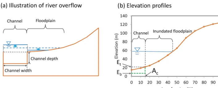
named MOSART-Inundation. Floodplain inundation dynam-ics were represented by macroscale inundation schemes in a few previous studies (Coe et al., 2008; Decharme et al., 2008; Getirana et al., 2012; Paiva et al., 2013a; Yamazaki et al., 2011). Those studies used relatively coarse compu-tation units with the area magnitude ranging from 100 to 10 000 km2. The main feature of their macroscale inundation schemes was that the water level–inundated area relationship for the computation unit was used to estimate flood extent. The inundation scheme of this study is similar to those of Yamazaki et al. (2011) and Getirana et al. (2012). In this scheme, each computation unit (a square grid cell or a sub-basin) has a main channel and a floodplain reservoir (Fig. 1a). Flooding water can spill out of the main channel and enter the floodplain reservoir or recede from the floodplain reservoir to the main channel. The lateral flow between adjacent compu-tation units is restricted to the main channel; namely, it is assumed that there is no water exchange between floodplains of different computation units. The water volume within each computation unit is used with an “elevation profile” (i.e., the relationship between the water stage and the inundated frac-tion of a computafrac-tion unit) to estimate the surface water area within the computation unit.
The brown solid line in Fig. 1b is the original elevation profile which is developed from all the elevations of the fine-resolution DEM within the computation unit. The channel area is implicitly included in the original elevation profile. Getirana et al. (2012) proposed an amended elevation profile in which the channel area was distinguished from the non-channel area. Their method was adopted in this study. It is assumed that the main channel consists of the lowest pixels of the DEM within a computation unit. Thus, the main chan-nel and the rest of the computation unit, including the flood-plain and the upland, are represented by the lower part and the upper part of the elevation profile, respectively (Fig. 1b). The dividing point corresponds to the fraction of channel area which is estimated as the product of the channel length de-rived from DEM data and the channel width calculated with empirical formulae in Sect. 2.5. The elevation of the dividing point corresponds to the channel bank top (Etin Fig. 1b). If
the channel cross-sectional shape is assumed to be a rectan-gle, the channel part of the elevation profile changes to follow the green dashed line in Fig. 1b. The channel bed elevation Ebequals the difference of the bank top elevationEtand the
channel depth, which is estimated in Sect. 2.5. The channel bed could be lower than the lowest DEM pixel of the compu-tation unit, as shown in Fig. 1b, because the DEM does not reflect the channel bed elevation.
loca-Figure 1.Illustrations of the macroscale inundation scheme:(a)illustration of river overflow;(b)elevation profiles of a computation unit (e.g., a grid cell or subbasin). The brown solid line is the original elevation profile. The green dashed line is the amended elevation profile (its non-channel part overlaps with the original elevation profile).Acis the fraction of the channel area in the computation unit,Etis the bank top elevation andEbis the channel bed elevation.
tions). Specifically, the exchange calculation is described as follows.
At the beginning of each time step, the total water volume Vtotal, including the channel water volume and floodplain
wa-ter volume, is compared with the channel storage capacity Schannel (i.e., the product of the channel length, width and
depth):
1. IfVtotal is less than or equal to Schannel, after the
ex-change process, all the water remains in the channel and the floodplain is not inundated according to the assump-tion of instantaneous exchange. That is, the river stage does not exceed the bank top (Etin Fig. 1b). When the
rectangular channel cross section is used, the surface water area does not change with the river stage and is always equal to the channel area (Fig. 1b).
2. IfVtotalis greater thanSchannel, after the exchange
pro-cess, the floodplain is inundated, and the water stage over the floodplain and the water stage in the channel are level due to the assumption of instantaneous ex-change, as shown by the blue water stage line in Fig. 1b. The final water stage can be derived fromVtotaland the
amended elevation profile becauseVtotal is equal to the
product of the computation unit area and the area of the polygon surrounded by the amended elevation profile, water stage line and they axis in Fig. 1b. The channel water volume is calculated as the product of the channel length, width and the water depth in the channel (i.e., the difference between the final water stage and the channel bed elevation Eb). The intersection of the final water
stage and the elevation profile indicates the fraction of the surface water area which includes the channel area and the inundated floodplain area.
The amount of the channel–floodplain water exchange is re-vealed by the change in the channel water volume during the exchange process and is used in the channel routing
com-putation described in Sect. 2.1. Specifically, the exchange amount is incorporated with the outflows from the tributary channels as the lateral inflow term in the continuity equation (i.e., Eq. 1). The lateral inflow term could be positive (the channel receives water) or negative (the channel loses wa-ter), depending on the amount and direction of the channel– floodplain exchange and the amount of tributary-channel out-flows.
2.3 Application in the Amazon Basin
The MOSART-Inundation model was applied to the entire Amazon Basin. The 3 arcsec HydroSHEDS DEM data de-veloped by the United States Geological Survey (USGS) was used in this study. The hydrologically conditioned Hy-droSHEDS DEM was used to generate the digital river net-work and subbasins. Relatively coarse-resolution subbasins were adopted, as MOSART-Inundation is intended for global earth system modeling which is constrained by computa-tional cost. The study domain of 5.89 million km2 was di-vided into 5395 subbasins (the average area was 1091.7 km2 and the standard deviation was 921.5 km2), which were used as computation units (Fig. 2a and b). Each subbasin had a main channel and the entire river network consisted of 5395 main channels (Fig. 2a). To ensure stable computation, the time-step size was determined based on the CFL condition and sensitivity tests. The time step of 1 min was used for all the simulations.
Figure 2.Basin discretization and model inputs.(a)The river network extracted from the DEM overlaps with 13 stream gauges: (a) Altamira; (b) Itaituba; (c) Fazenda Vista Alegre; (d) Canutama; (e) Gavião; (f) Acanaui; (g) Serrinha; (h) Cachoeira da Porteira; (i) Santo Antônio do Içá; (j) Itapeua; (k) Manacapuru; (l) Jatuarana and Careiro; (m) Óbidos. Panel(b)indicates the magnified quadrat. The thin (thick) black lines mark boundaries between subbasins (subregions). Panel(c)indicates the delineation of 10 subregions (including 9 tributary subregions and the main stem subregion indicated by dark green color). Panel(d)indicates average DEM deductions at each subbasin for alleviating vegetation-caused biases;(e)the corrected DEM;(f) averaged elevation profiles based on the original and corrected DEMs;(g)channel widths;(h)channel depths; and(i)Manning roughness coefficients of channels.
subregion and the remaining five large catchments were in-corporated into their adjacent tributary subregions. This way, nine tributary subregions were delineated. Lastly, all the small tributary catchments and the area draining directly to the main stem were aggregated to be the 10th subregion (i.e., the main stem subregion).
The inputs of surface and subsurface runoff, which were of 1◦resolution, were produced by the ISBA land surface model
2.4 Vegetation-caused biases in DEM
In the previous section, it is mentioned that the digital river network and subbasins were derived from the hydrologically conditioned HydroSHEDS DEM. However, this conditioned DEM was not suitable for representing floodplain topogra-phy and generating elevation profiles. In the DEM condi-tioning process, the elevation values of pixels for river chan-nels and their buffer zones were lowered by non-negligible amounts that could, for example, be larger than 20 m in the lower main stem area of the Amazon Basin. Thus, the chan-nels and their adjacent areas in the conditioned DEM could hold more water than the actual counterparts, which would lead to underestimation of flood extent. Therefore, the void-filled HydroSHEDS DEM, which was not altered by the con-ditioning process, is more appropriate for use in generating the elevation profiles.
However, the void-filled HydroSHEDS DEM was derived from the SRTM data, so it inherited the vegetation-caused bi-ases. Before being used for producing elevation profiles, the void-filled HydroSHEDS DEM was processed to alleviate the biases caused by vegetation. The vegetation height data with ∼1 km resolution developed by Simard et al. (2011) was used. For vegetated areas, the original void-filled DEM represented elevations of locations within the vegetation canopy. Thus, part of the vegetation height needed to be deducted from the original elevation. Baugh et al. (2013) found that deducting 50–60 % of the vegetation height of the Simard et al. (2011) data from the original DEM achieved the greatest improvements to hydrodynamic model accuracy in the Amazon floodplain. A deduction ratio of 50 % was used for the vegetated area in this study.
The resolution of the vegetation height data was coarser than that of the DEM data. It might not be appropriate to assume a uniform vegetation height for all the DEM pixels within the grid cell of the vegetation height dataset. Hess et al. (2003, 2015a) developed a high-resolution (3 arcsec) land cover dataset for floodplains (or wetlands) located in the low-land Amazon Basin (i.e., areas with elevations lower than 500 m). This land cover dataset was used in our DEM cor-rection process. In the floodplains of the lowland Amazon Basin, vegetation height removal was conducted differently for different land cover classes. For DEM pixels with forest or woodland classes, 50 % of the vegetation height was de-ducted from the original DEM. In the high-resolution land cover dataset, shrubs were defined to be less than 5 m tall (Junk et al., 2011). Thus, for DEM pixels with shrubs, the vegetation height was determined by the vegetation height data, but with an upper limit of 5 m. After this correction, the elevations were lowered by 50 % of the vegetation heights for shrub DEM pixels. For DEM pixels with other land cover classes (open water, bare soil, etc.), the elevations were not modified. For areas outside of the floodplains of the low-land basin, a uniform vegetation height was applied for all the DEM pixels within each vegetation height pixel. This
ap-proximation was not expected to have obvious effects on in-undation modeling since most inin-undation occurred within the floodplains of the lowland basin.
The DEM correction obviously changed the topographic features in the DEM data. The average elevation deduction in each subbasin ranged from 0 to 21 m (Fig. 2d). After the DEM correction, the average elevation in each subbasin ranged from 0 to 4772 m (Fig. 2e). For all the subbasins, the ratio of the average elevation deduction to the subbasin ele-vation difference (i.e., the difference between the highest and lowest elevations in the subbasin) ranged from 0 to 52.9 % (average: 9.2 %; standard deviation: 7.1 %). The average el-evation profile of the Amazon Basin was generated for the original DEM and corrected DEM, respectively (Fig. 2f). At first, the normalized elevation profile was produced for each subbasin. For each DEM pixel within a subbasin, the eleva-tion relative to the lowest pixel of the subbasin was divided by the subbasin elevation difference to give the normalized elevation, which was used to generate the normalized ele-vation profile. Then, the normalized eleele-vation profiles of all subbasins were averaged to give the average elevation profile of the entire basin. Figure 2f illustrates that the DEM pro-cessing evidently lowers the average elevation profile.
O’Loughlin et al. (2016) estimated the vegetation-caused biases in the SRTM DEM data based on vegetation height data, canopy density data and the distribution of five cli-matic zones (i.e., tropical, arid, temperate, cold and po-lar). They created the first global bare-earth high-resolution (3 arcsec) DEM from the SRTM DEM data. They compared their method with the static correction method (i.e., estimat-ing the vegetation-caused bias as the product of vegetation height and a fixed percentage) used by Baugh et al. (2013) and this study, and noted that the static correction method was effective but moderately worse than their method.
2.5 Channel geometry
as follows:
w=1.956A0.413 (A <10 000 km2) (4) w=0.403A0.600 (A≥10 000 km2) (5)
d=0.245A0.342, (6)
wherewis channel width (unit: m);dis channel depth (unit: m); and A is upstream drainage area (unit: km2). Beigh-ley and Gummadi (2011) showed that the channel cross-sectional dimensions estimated from their channel geome-try formulae agreed well with those from the formulae by Coe et al. (2008). Based on extensive river morphology data obtained from stations spread throughout the Amazon and Tocantins basins, Coe et al. (2008) derived the general chan-nel geometry formulae for the Amazon Basin and, in their formulae, channel cross-sectional dimensions were also ex-pressed as power functions of upstream drainage area.
The channel geometry formulae of Beighley and Gum-madi (2011) were obtained through regression analysis of data from 82 locations over the Amazon Basin and reflected the average feature of the basin. Directly applying the same formulae and parameters to the entire basin could cause large biases in the estimated channel cross-sectional dimensions for some subregions. In order to reduce those biases, in this study, the coefficients in the basin-wide channel geometry formulae of Beighley and Gummadi (2011) were adjusted for the majority of the 10 subregions (Fig. 2c) based on channel cross-sectional dimensions of local locations. The 82 streamflow gauging locations scattered over the Amazon Basin and each subregion contained a few streamflow gaug-ing locations. For the streamflow gauggaug-ing locations of the same subregion, the root mean square error (RMSE) between the channel cross-sectional dimensions estimated with the channel geometry formulae and the corresponding dimen-sions presented in Beighley and Gummadi (2011) could be calculated. During the adjustment process, the coefficient of the channel geometry formula (i.e., 1.956, 0.403 or 0.245 in Eqs. 4–6) was multiplied by a factor to reduce the RMSE. The factor values for the 10 subregions are listed in Table 1. The ranges for the channel width and depth of each subbasin are shown in Fig. 2g and h, respectively.
It is worth mentioning that Paiva et al. (2013a) also ac-counted for spatial variability of channel geometry formulae and used various coefficients in their formulae for six zones of the Amazon Basin. In this study, we used both the basin-wide channel geometry formulae and the diverse formulae for various subregions and investigated the effects of refin-ing channel geometry on modeled surface water dynamics.
In order to convert the calculated channel water depths to river stages, we estimated the riverbed elevations by using the following equation, since observed data were not available:
Ec=Emouth+
n X
i=1 LiSi+
1
2LcSc, (7)
where Ec is the average riverbed elevation of the current
channel (unit: m); Emouth is the riverbed elevation at the
mouth of the Amazon River (unit: m);nis the total number of downstream channels;Li is the flow length of a down-stream channeli(unit: m);Si is the average riverbed slope of a downstream channeli (dimensionless);Lc is the flow
length of the current channel (unit: m) andSc is the
aver-age riverbed slope of the current channel (dimensionless). Emouth is assumed to be the negative channel depth at the
mouth of the Amazon River, which is calculated with Eq. (6). The riverbed slopes were extracted from the DEM and could contain uncertainties since the DEM did not reflect the actual riverbed elevations.
2.6 Manning roughness coefficients for channels The Manning roughness coefficient for channels reflects the resistance to water flows in channels and is determined by many factors, such as roughness of riverbed and riverbank, shape and size of channel cross sections and channel mean-derings. In general, within a basin, these factors have con-siderable spatial heterogeneities. Therefore, it is more rea-sonable to use spatially varying coefficients estimated based on these factors than using a constant coefficient. However, distributed hydrologic modeling requires a channel Man-ning coefficient for each subbasin. It is not realistic to sep-arately estimate each of the Manning coefficients given the lack of information. For continental-scale studies, the river network consists of river channels of distinct magnitude or-ders. Riverbed resistance plays a relatively smaller role in water flows of larger channels. Assuming that the Manning coefficient decreases linearly with the channel top width, Decharme et al. (2010) showed that the assumed relationship produced acceptable variation in flow velocity in a global ap-plication of the ISBA-TRIP continental hydrologic modeling system. Getirana et al. (2012) expressed the Manning coeffi-cient as a power function of the channel depth in their study of inundation dynamics in the Amazon Basin. In our study, the Manning coefficient also depended on the channel depth and was estimated using the following function:
n=nmin+(nmax−nmin)
hmax−h hmax−hmin
, (8)
where the maximum Manning coefficient nmax is for the
channel with the shallowest channel depth and the minimum Manning coefficientnminis for the channel with the largest
channel depth. Following Getirana et al. (2012),nmax and nmin were set as 0.05 and 0.03, respectively. In addition, a
few other studies of the Amazon Basin adopted similar val-ues around the range of 0.03–0.05 for the Manning coeffi-cient (Beighley et al., 2009; Paiva et al., 2013a; Yamazaki et al., 2011). In Eq. (8),hmaxandhminare the maximum and
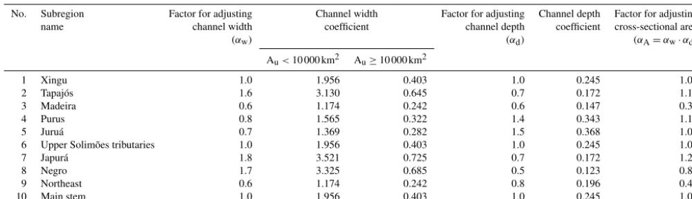
cur-Table 1.Coefficients in channel geometry formulae for the 10 subregions.
No. Subregion Factor for adjusting Channel width Factor for adjusting Channel depth Factor for adjusting
name channel width coefficient channel depth coefficient cross-sectional area
(αw) (αd) (αA=αw·αd)
Au<10 000 km2 Au≥10 000 km2
1 Xingu 1.0 1.956 0.403 1.0 0.245 1.00
2 Tapajós 1.6 3.130 0.645 0.7 0.172 1.12
3 Madeira 0.6 1.174 0.242 0.6 0.147 0.36
4 Purus 0.8 1.565 0.322 1.4 0.343 1.12
5 Juruá 0.7 1.369 0.282 1.5 0.368 1.05
6 Upper Solimões tributaries 1.0 1.956 0.403 1.0 0.245 1.00
7 Japurá 1.8 3.521 0.725 0.7 0.172 1.26
8 Negro 1.7 3.325 0.685 0.5 0.123 0.85
9 Northeast 0.6 1.174 0.242 0.8 0.196 0.48
10 Main stem 1.0 1.956 0.403 1.0 0.245 1.00
Note:Auis the upstream drainage area.
rent channel. The spatial distribution of the channel Manning coefficient is shown in Fig. 2i.
In this study, the function of the Manning coefficient (i.e., Eq. 8) was compared to those of Decharme et al. (2010) and Getirana et al. (2012). In general, compared to the equations of the two previous studies, Eq. (8) gave smaller Manning coefficients and resulted in better simulation of hydrographs, which suggested that Eq. (8) was more appropriate for the simulations of this study.
2.7 Control simulation
The aforementioned factors could have important impacts on modeling surface hydrology of the Amazon Basin. We con-figured a control simulation (abbreviated as CTL) using the preferred methodologies for five aspects: (1) the inundation scheme was turned on; (2) vegetation-caused biases in the DEM data were alleviated; (3) the basin-wide channel geom-etry formulae were refined for different subregions; (4) the Manning coefficient varied with the channel size; and (5) the diffusion wave method was used to represent river flow in channels. The control simulation was run for 14 years (1994– 2007) and the results of 13 years (1995–2007) were eval-uated against gauged streamflow data and remotely sensed river stage and inundation data.
3 Model evaluation 3.1 Streamflow
The observed daily streamflow data for model evaluation were from 13 stream gauges operated by the Brazilian Wa-ter Agency. A total of 8 of the 13 gauges either control the major area of a tributary subregion or are typical gauges in their tributary subregions. None of the 13 gauges are located in the tributary subregion “upper Solimões tributaries” in the western Amazon Basin. Most of this subregion is controlled by the Santo Antônio do Içá gauge at the upper main stem.
The remaining four gauges are located along the middle or lower main stem.
The simulated daily streamflow results were compared with the observed data for a 12-year period (1995–2006) at the 13 stream gauges (Fig. 3). The Nash–Sutcliffe effi-ciency coefficient (NSE) and the relative error of mean an-nual streamflow (RE) were calculated for each gauge (Fig. 3). For the majority of the 13 gauges, daily streamflow val-ues were reproduced fairly well. The NSE value is higher than 0.62 at seven gauges. The four gauges with NSE values lower than 0.5 have high absolute values of RE (i.e.,>0.20), which suggests that large biases in runoff inputs for the ar-eas upstream of those gauges degrade the streamflow results. Overall, runoff inputs have large negative biases in the west-ern portion of the Amazon Basin and large positive biases in the southern and southeastern portions. The runoff biases could be caused by errors in the precipitation forcing dataset or errors in the land surface water fluxes calculated by the land surface model (e.g., canopy evaporation, plant transpi-ration and soil evapotranspi-ration). In general, the simulated stream-flow results are comparable to those of a few previous stud-ies (e.g., Getirana et al., 2012; Yamazaki et al., 2011) and slightly worse than those of Paiva et al. (2013a).
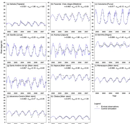
3.2 River stage
Figure 3.Comparison between modeled and observed daily streamflow for a 12-year period (1995–2006) at 13 stream gauges (the cor-responding subregion names are shown in the brackets):(a)Altamira (Xingu);(b)Itaituba (Tapajós);(c)Fazenda Vista Alegre (Madeira);
(d)Canutama (Purus);(e)Gavião (Juruá);(f)Acanaui (Japurá);(g)Serrinha (Negro);(h)Cachoeira da Porteira (northeast);(i)Santo Antônio do Içá (main stem);(j)Itapeua (main stem);(k)Manacapuru (main stem);(l)Jatuarana and Careiro (main stem);(m)Óbidos (main stem). The Nash–Sutcliffe efficiency coefficient and the relative error of mean annual streamflow are indicated at the upper right corner of each panel. Figure 2a shows the stream-gauge locations.
uncertainties in the riverbed elevation are expected due to the large uncertainties in the riverbed elevation at the mouth and the riverbed slopes. Therefore, the simulated river stage of a channel is negatively affected by parameter biases of downstream channels and cannot be directly compared to the observations. The timing and magnitude of simulated river-stage fluctuations were compared to those of observed data. The comparison was conducted at the daily scale during a 6-year period (2002–2007) for the 11 subbasins containing the 11 virtual stations (Fig. 4). For better visual comparison,
over-estimated for the subbasins of four gauges (i.e., Canutama, Acanaui, Serrinha and Santo Antônio do Içá). The standard deviation of the simulated river stages is much larger than that of the observed data, which could be primarily due to a few reasons: (1) overestimation of streamflow peaks (e.g., Canutama and Acanaui), which could be caused by biases of runoff inputs or underestimation of flood extent in the up-stream area; (2) uncertainties in model parameters of chan-nel cross-sectional geometry, chanchan-nel Manning coefficients, etc. Overall, in terms of the timing and magnitude of fluctu-ations, the modeled river stages of this study are comparable to those reported in some previous investigations (Coe et al., 2008; Getirana et al., 2012; Paiva et al., 2013a).
3.3 Flood extent
The simulated flood extent results were evaluated using the Global Inundation Extent from Multi-Satellites (GIEMS) data (Papa et al., 2010; Prigent et al., 2007, 2012). The GIEMS data contained monthly surface water area during a 15-year period (1993–2007) for each of the land pixels of equal area (i.e., 773 km2). The area-weighted averaging method was used to convert the grid-based surface water ex-tent data to subbasin-based data for use in this study. Lake area was not deducted from the GIEMS data because in the Amazon Basin the lakes usually were located in the low por-tion of one subbasin and the simulated inundated area also contained lake areas.
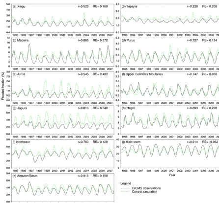
The simulated monthly flood extent results (including channel surface area and flooded area over floodplains) were compared to the GIEMS data during a 13-year period (1995–2007) for 10 subregions and the entire Amazon Basin (Fig. 5). The Pearson correlation coefficient and the mean annual relative difference between the simulated flood extent results and the observations were calculated. The timing of inundation was reproduced well for most area of the Ama-zon Basin: the Pearson correlation coefficient was equal to or larger than 0.727 at 7 of the 10 subregions and the entire basin. The mean annual value of simulated flood extent was comparable to that of the GIEMS observations for a major portion of the basin: the absolute value of the mean annual relative difference was less than 0.23 at 7 of the 10 subre-gions and the entire basin.
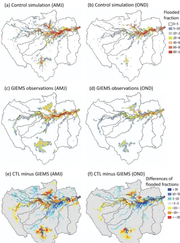
The spatial pattern of simulated flood extent was also com-pared to that of the GIEMS observations for high-water and low-water seasons (Fig. 6). For each subbasin, the simu-lated or observed flooded fractions of 13 years (1995–2007) were averaged for the high-water season (April, May and June) and low-water season (October, November and De-cember), respectively. Both the observations and the simu-lated results show evident inundation in the regions near the middle and lower main stem. The observed inundation in the upper Madeira subregion and middle Negro subregion is par-tially captured by the model. The comparison also shows spa-tially varying differences between the modeled and observed
flood extent (Fig. 6e and f). The modeled flood extent ex-ceeds the observations in the lower Madeira subregion near the main stem and around the major reaches in the middle Negro subregion. At the same time, the modeled flood extent is lower than the observations for some subbasins in the main stem, upper Madeira, upper Solimões and middle Negro sub-regions.
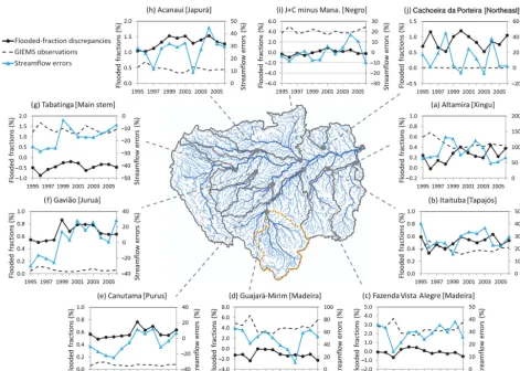
The aforementioned discrepancies between the simulated flood extent and the GIEMS data could be related to biases of runoff inputs, which have important effects on the stream-flow simulation, as noted earlier. The runoff biases (i.e., the differences between runoff inputs and “actual” runoff) in the upstream area of a stream gauge could be inferred from the long-term mean streamflow errors. Comparing the annual streamflow errors to the flood extent errors upstream of the gauge from the year 1995 to 2006 (Fig. 7) shows that runoff biases could be the partial cause for the flood extent discrep-ancies. For 3 of the 10 gauges (i.e., (b) Itaituba, (g) Tabatinga and (h) Acanaui), the upstream flood extent discrepancies are consistent with the streamflow errors (i.e., both are posi-tive or negaposi-tive) in all 12 years. For the other seven gauges, upstream flood extent discrepancies and streamflow errors are consistent for some years, but contradictory for other years. This result suggests that flood extent discrepancies were also caused by other factors such as (1) uncertainties in model parameters including floodplain topography, chan-nel cross-sectional geometry, chanchan-nel Manning coefficients, the riverbed slope, etc.; (2) surface water bodies (e.g., lakes and swamps) not represented by the model that were lumped into the inundated floodplains; (3) subsurface processes and wetlands sustained by groundwater that were not simulated; and (4) inundation that could be underestimated or overesti-mated in the GIEMS data which were of comparatively low resolution (Hess et al., 2015a; Prigent et al., 2007). The ef-fects of model parameters (including floodplain topography, channel cross-sectional geometry and channel Manning co-efficients) on the inundation results were investigated in the sensitivity study.
Figure 4.Comparison of modeled daily river stages with the observations for a 6-year period (2002–2007) at the subbasins containing or close to 11 of the 13 stream gauges (the corresponding subregion names are shown in the brackets):(a)Itaituba (Tapajós);(b)Fazenda Vista Alegre (Madeira);(c)Canutama (Purus);(d)Gavião (Juruá);(e)Acanaui (Japurá);(f)Serrinha (Negro);(g)Santo Antônio do Içá (main stem);(h)Itapeua (main stem);(i)Manacapuru (main stem);(j)Jatuarana and Careiro (main stem);(k)Óbidos (main stem). The Pearson correlation coefficient between modeled river stages and the observations, as well as standard deviation for modeled and observed river stages, is indicated in each panel. The simulated river stages are shifted to coincide with the observations for better visual comparison (please see Sect. 3.2 for the detailed explanation).
4 Sensitivity study
A sensitivity study was carried out to investigate the roles of the following factors in modeling of surface hydrology of the Amazon Basin: (1) representing floodplain inundation; (2) alleviating vegetation-caused biases in the DEM; (3) re-fining channel geometry; (4) adjusting Manning coefficients; and (5) accounting for backwater effects. Six scenario simu-lations were designed so that for each simulation only one of the above five factors was changed from the control simula-tion described in Sect. 2.7 (Table 2). All simulasimula-tions were run
for 14 years (1994–2007) and the results of 13 years (1995– 2007) were analyzed. The results of the control simulation were compared with those of each scenario simulation to sep-arately examine the impacts of each factor on the modeled streamflow, river stages and inundation.
Figure 5.Comparison of modeled monthly flood extent to the GIEMS satellite observations during a 13-year period (1995–2007) for 10 subregions and the entire Amazon Basin:(a)Xingu;(b)Tapajós;(c)Madeira;(d)Purus;(e)Juruá;(f)upper Solimões tributaries;(g)Japurá;
(h)Negro;(i)northeast;(j)main stem;(k)Amazon Basin. The Pearson correlation coefficient between the modeled and observed monthly flood extent and the relative error of mean annual flood extent are indicated in each panel.
Table 2.Setup of seven simulations.
No. Inundation DEM Channel cross- Manning roughness Method for representing Abbreviations scheme sectional geometry coefficients of channels river flow
1 On Corrected Refined Spatially varying Diffusion wave method CTL
2 Off Corrected Refined Spatially varying Diffusion wave method NoInund
3 On Original Refined Spatially varying Diffusion wave method OriDEM
4 On Corrected No refining Spatially varying Diffusion wave method OriSec
5 On Corrected Refined 0.03 Diffusion wave method n003
6 On Corrected Refined 0.04 Diffusion wave method n004
Figure 6.Average spatial patterns of flooded fractions for all subbasins during 13 years (1995–2007):(a)results of the control simulation in the high-water season (AMJ – April, May and June);(b)results of the control simulation in the low-water season (OND – October, November and December);(c)GIEMS observations in the high-water season;(d)GIEMS observations in the low-water season;(e)differences between the control simulation and GIEMS observations in the high-water season; and(f)differences between the control simulation and GIEMS observations in the low-water season.
inundation scheme in improving the modeled streamflow and river stages (Sect. 4.1).
The original HydroSHEDS DEM data without the correc-tion of vegetacorrec-tion-caused biases were used in the third simu-lation (abbreviated as OriDEM); the basin-wide channel ge-ometry formulae were not refined for different subregions and were directly used for the entire basin in the fourth
simu-lation (abbreviated as OriSec). The results of these two sim-ulations were contrasted with those of the control simulation to show the effects of geomorphological parameters on mod-eling surface water dynamics (Sect. 4.2 and 4.3).
et al., 2011). A constant Manning coefficient of 0.03 and 0.04 was used in the fifth and sixth simulations, respectively (abbreviated as n003 and n004). The diffusion wave method was replaced by the kinematic wave method for representing water flow through channels in the seventh simulation (ab-breviated as KW). These three simulations were compared with the control simulation to reveal the impacts of river flow representations on modeled surface hydrology (Sect. 4.4 and 4.5).
In the comparisons between the control simulation and the contrasting scenario simulations, we examined the model re-sults of various locations spread over the Amazon Basin, in-cluding streamflow at 13 major main stem or tributary gauges (Fig. 8), river stages near 11 major gauges (Fig. 9), the main stem water surface profile (Fig. 10), inundation of 10 subre-gions (Fig. 11) and spatial patterns of inundation differences for the entire basin (Fig. 12). In the following discussions, Figs. 8–12 are used jointly to reveal the impacts of the five factors on surface water dynamics.
4.1 Representing floodplain inundation
The comparison of streamflow results between the control simulation CTL and the simulation NoInund shows that in-corporating the inundation scheme evidently improves the modeled streamflow. More specifically, streamflow peaks are reduced and delayed, and the streamflow hydrographs be-come smoother (Fig. 8). The impacts are especially promi-nent in the subregions with evident inundation (e.g., Fig. 8c) and at the gauges in the middle and lower main stem (Fig. 8j– m). This result demonstrates that floodplains play a signifi-cant role in regulating streamflow of the Amazon Basin.
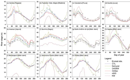
Figure 9 shows that incorporating the inundation scheme has prominent impacts on the modeled river stages of most of the 11 subbasins examined in this study: the river-stage peaks are attenuated and delayed, and the river-stage tim-ing and fluctuation magnitude are improved. The impacts are most obvious in the subregions with evident inundation (e.g., Fig. 9b) and in the middle and lower main stem (Fig. 9h–k). One exception is that the large improvement of river stages near the Itaituba gauge (Fig. 9a) is primarily caused by the improvement of main stem river stages because the Itaituba gauge is close to the lower main stem and its river stages are influenced by the main stem through backwater effects.
Including the inundation scheme brings about changes of the main stem water surface profile and the changes are more evident in the rising-flood season than in other sea-sons (Fig. 10). In the rising-flood season, the average water surface profile is lowered for the entire main stem section examined here and the large river-stage differences occur in the middle main stem with magnitude up to more than 5 m (Fig. 10a). In the high-water season, the average water sur-face profile is also lowered (Fig. 10b). However, Fig. 10c shows that in the falling-flood season the main stem river stages are raised because water stored in the floodplains
re-turns to the river channels. Similar to the rising-flood season, large river-stage differences appear in the middle main stem with a magnitude of about 3 m. In the low-water season, the average water surface profile is slightly lowered (Fig. 10d). It should be noted that the main stem river stages are first raised and then lowered during the 3 months (Fig. 9h–k).
The above comparisons and analyses reveal that incorpo-rating the inundation scheme into hydrologic modeling has prominent impacts on the simulated surface hydrology in the Amazon Basin and significantly improves both the stream-flow and the river-stage hydrographs, especially at reaches whose upstream area involves large floodplains. This result suggests that floodplain inundation is an important compo-nent of the surface water dynamics in the Amazon Basin and should be represented in hydrologic modeling for this basin. Some previous studies also examined and reported the im-pacts of representing the floodplain inundation on the mod-eled surface hydrology in the Amazon Basin (Getirana et al., 2012; Paiva et al., 2013a; Yamazaki et al., 2011). Yamazaki et al. (2011) showed the impacts of floodplain inundation on the streamflow, water depths and flow velocities at the Óbidos gauge (in their Fig. 5) and the main stem water surface pro-file (in their Fig. 7). Getirana et al. (2012) demonstrated the effects of floodplain inundation on streamflow of a few main stem gauges (in their Fig. 16). When investigating the im-pacts of floodplain inundation on surface hydrology, these two studies used the kinematic wave river routing method that could not represent the important backwater effects in the Amazon Basin, while we used the diffusion wave river routing method that captured backwater effects. Backwater effects were also represented in the dynamic wave river rout-ing method used by Paiva et al. (2013a) when they studied the impacts of floodplain inundation on streamflow of a few major tributary or main stem gauges including Óbidos and Manacapuru (in their Table 2 and Fig. 14). Besides stream-flow, in this study, we also examined and revealed the promi-nent impacts of floodplain inundation on the river stages near 11 major gauges or along the main stem.
4.2 Correcting DEM
The vegetation-caused biases in the HydroSHEDS DEM data were alleviated via DEM correction. This lowered the flood-plain elevations and changed the slope of the elevation pro-file, which could lead to changes in simulated flood extent. Figure 11 shows that the DEM correction increases flood ex-tent in all 10 subregions. The increase of inundation post-pones and lowers streamflow peaks in the downstream chan-nels, especially in the middle and lower main stem (Fig. 8j– m).
el-Figure 7.Streamflow errors and the flood extent discrepancies (i.e., the differences between simulated flood extent and the GIEMS data) in the area upstream of the gauge for 10 gauges at the annual scale during 12 years (1995–2006). Streamflow of the Negro subregion(i)is approximated by the streamflow difference between the Jatuarana and Careiro gauge and the Manacapuru gauge. The upstream area of each gauge is enclosed by the gray lines (or brown dotted lines for the Guajará-Mirim gauge) in the basin map.
evated in the falling-flood and low-water seasons (Fig. 10c and d), with a magnitude up to about 1 m.
Figure 12a and b show that DEM correction leads to in-undation changes in many subbasins: while flood extent is mostly enlarged, DEM correction also could increase the slope of the elevation profile in some subbasins and reduce flood extent.
The vegetation-caused biases in DEM data were alleviated with various approaches in a few previous studies modeling the surface hydrology in the Amazon Basin (Baugh et al., 2013; Coe et al., 2008; Getirana et al., 2012; Paiva et al., 2011, 2013a; Wilson et al., 2007; Yamazaki et al., 2011). Most of these studies did not examine and explicitly report the effects of the DEM correction on the modeled results. Baugh et al. (2013) demonstrated that alleviating vegetation-caused biases in DEM could improve the modeled water levels and inundation over floodplains adjacent to a 280 km reach of the central Amazon (in their Figs. 2 and 5).
4.3 Refining channel geometry
Adjusting channel cross-sectional geometry could evidently affect the simulated surface water area (Fig. 11) and the changes are caused by two mechanisms: (1) reducing the channel cross-sectional area, which is equivalent to reduc-ing channel conveyance capacity, could increase flooded area over floodplains, and vice versa; (2) broadening the channel width, hence increasing channel surface area, and vice versa. The nine tributary subregions can be placed in five categories according to the changes of channel cross-sectional area, the channel width and the total surface water area (Table 3). The channel geometry of the main stem is not adjusted. The inun-dation changes in the tributary subregions affect streamflow in the main stem and slightly delay and attenuate the inunda-tion peak there (Fig. 11j).
Figure 8.Observed and modeled daily streamflow of the year 2005 at 13 stream gauges. The setup of the six simulations is described in Table 2: CTL – control simulation; NoInund – without inundation scheme; OriDEM – using the original DEM (with vegetation-caused biases); OriSec – using basin-wide channel geometry formulae; n003 – using a uniform Manning roughness coefficient (i.e., 0.03) for all the channels; KW – using the kinematic wave method to represent river flow.
Table 3.Refining the channel cross-sectional geometry affects inundated area in tributary subregions.a
Category Cross-sectional Inundated area Channel Channel Total surface Subregions areab over floodplains widthc area water aread
A − + + + + (h) Negro
B − + − − + (c) Madeira; (i) northeast
C + − + + + (b) Tapajós; (g) Japurá
D + − − − − (d) Purus; (e) Juruá
E No refining No change No refining No change No change (a) Xingu; (f) upper Solimões tributaries
Note:a“+” means increase; “−” means decrease.bThis variation depends on the factorαAin Table 1:αA>1: “+”;αA<1: “–”;αA=1: “No refining”.cThis variation depends on the factorαwin Table 1:αw>1: “+”;αw<1: “–”;αw=1: “No refining”.dThis change is shown by inundation results in Fig. 11.
(Table 1), which evidently increases inundation in this sub-region (Fig. 11c). A similar phenomenon is observed at the Cachoeira da Porteira gauge in the northeast subregion (Fig. 8h), where the channel cross-sectional area is multi-plied by a factor of 0.48. Inundation changes caused by re-fining channel geometry in other subregions are
compara-tively smaller than those of the Madeira and northeast sub-regions, and do not result in significant alterations in stream-flow (Fig. 8).
Figure 9.Observed and modeled river stages at the daily scale in the year 2005 for the subbasins containing or close to 11 of the 13 stream gauges. The setup of the six simulations is described in Table 2: CTL – control simulation; NoInund – without inundation scheme; OriDEM – using the original DEM (with vegetation-caused biases); OriSec – using basin-wide channel geometry formulae; n003 – using a uniform Manning roughness coefficient (i.e., 0.03) for all the channels; KW – using the kinematic wave method to represent river flow.
not straightforward. For instance, reducing the channel width could raise the river stage and hence increase the flow veloc-ity or inundation, which, in turn tend to lower the river stage (Fig. 13). The simulated results of this study show that, in most circumstances, reducing the channel width raises the river stage of the local channel (Fig. 9b, c and d) and vice versa (Fig. 9e and f). In Fig. 9a, this rule does not apply from about day 160 to 350, which could be caused by backwater effects: the river stage of this channel is influenced by that of the main stem section downstream of the Óbidos gauge.
Channel geometry changes could also influence river stages of remote downstream channels. The channel mor-phology of the main stem is not adjusted. Thus, the river stage changes along the main stem are caused by inundation changes in the upstream area. The channel geometry adjust-ment of this study increases inundation in the major portion of the Amazon Basin, which influences river stages along the main stem, particularly in the middle reaches: the river stages averaged over 3 months are lowered in the rising-flood and high-water seasons (Fig. 10a and b) and elevated in the falling-flood and low-water seasons (Fig. 10c and d), with a magnitude up to about 1 m. The phenomenon can also be observed in Fig. 9h–k.
The sensitivities of modeled surface hydrology to chan-nel geometry were also investigated by some former
Figure 10.Modeled average river surface profiles along the middle and lower main stem in the four seasons of the year 2005:(a)JFM (January, February and March; the period of rising flood);(b)AMJ (April, May and June; the period of high water);(c)JAS (July, August and September; the period of falling flood); and (d)OND (October, November and December; the period of low water). Results of six simulations are shown. The four stream-gauge locations are labeled on thexaxis: Ita – Itapeua; Man – Manacapuru; J+C – Jatuarana and Careiro; Obi – Óbidos. Riverbed slopes(e)and Manning roughness coefficients(f)along the main stem are also shown. In the panel(f), the solid curve shows spatially varying Manning coefficients used in five simulations; the dotted line shows the uniform Manning coefficient of 0.03 used in the simulation n003.
analyzed with approaches of which some were different from those of the former studies.
4.4 Varying Manning roughness coefficients
A few studies for the Amazon Basin (e.g., Paiva et al., 2013a; Yamazaki et al., 2011) revealed some sensitivities of surface hydrology to the Manning coefficient. Yamazaki et al. (2011) perturbed the Manning coefficient by a uniform percentage for all the channels and examined the effects on streamflow of the Óbidos gauge and the flooded area over the central Amazon region (in their Fig. 13). Using a similar approach,
Figure 11.Observed and modeled average monthly flood extent of 13 years (1995–2007) for the 10 subregions and the entire Amazon Basin. Setup of the five simulations is described in Table 2: CTL – control simulation; OriDEM – using the original DEM (with vegetation-caused biases); OriSec – using basin-wide channel geometry formulae; n003 – using a uniform Manning roughness coefficient (i.e., 0.03) for all the channels; KW – using the kinematic wave method to represent river flow.
The streamflow Nash–Sutcliffe efficiency coefficients (NSEs) of CTL were compared with those of n003 and n004 (Table 4). The NSEs of CTL are higher than those of n004 at 10 of the 13 gauges (except Fazenda Vista Alegre, Itapeua and Manacapuru) and higher than those of n003 at 12 of the 13 gauges (except Óbidos). These results suggest that the spatially varying Manning coefficients are more appropriate than the uniform Manning coefficient of 0.03 or 0.04 for the simulations of this study.
The spatially varying Manning coefficients range from 0.03 to 0.05 and are equal to or larger than the Manning coefficient of 0.03. The spatially varying Manning cients result in larger flood extent than the uniform coeffi-cient of 0.03 (Fig. 11). The larger Manning coefficoeffi-cient leads to the lower flow velocity, larger wet cross-sectional area and thereby higher river stage (Fig. 9), which increase local in-undation, as well as upstream inundation due to backwater effects. Inundation increases in the upstream area postpone and attenuate flood waves at the downstream gauges (Fig. 8). Increases of the Manning coefficients not only affect lo-cal and upstream river stages as discussed above but also influence downstream river stages. Inundation increases in the upstream area have an impact on streamflow rates and hence river stages in the downstream channels. Therefore, river stages are influenced by not only downstream and
lo-cal Manning coefficients but also upstream Manning coeffi-cients. Figure 9 shows that the Manning coefficient increases result in rise of river stages in most circumstances, which suggests that the local and downstream effects play a domi-nant role: increases of Manning coefficients reduce flow ve-locities, enlarge wet cross-sectional area and hence elevate river stages. However, in the lower main stem, the upstream effects may overwhelm the local and downstream effects. For instance, Fig. 9k shows that, during the rising-flood period (before about the day 150), the Manning coefficient increases reduce river stages at the Óbidos gauge. The main reason is that the larger Manning coefficient promotes inundation in the upstream area, which results in smaller streamflow rates in the lower main stem for the rising-flood period.
4.5 Backwater effects
Figure 12.Differences in subbasin flooded fractions averaged during 13 years (1995–2007) between the control simulation (CTL) and the four contrasting simulations (i.e., OriDEM, OriSec, n003 and KW) for the high-water season (AMJ – April, May and June) and low-water season (OND – October, November and December):(a, b): CTL minus OriDEM;(d, e): CTL minus OriSec;(g, h): CTL minus n003;(j, k): CTL minus KW. Panel(c)shows DEM differences (CTL minus OriDEM);(f)categories of cross-section changes for the 10 subregions;
(i)Manning coefficient differences (CTL minus n003).
kinematic wave method that could not represent backwater effects. The results of the control simulation were compared with those of the simulation KW to reveal backwater effects on surface water dynamics.
4.5.1 Backwater effects on flood extent
backwa-Decreasing the channel width
Increasing the water depth assuming no change in the streamflow rate and flow velocity
Increasing the friction slope (Eq. 1)
Increasing the hydraulic radius (Eq . 2), which is
approximately equal to the water depth for very wide channels
Increasing the flow velocity (Eq. 2)
Decreasing the wet cross-sectional area, assuming no change in the streamflow rate
Increasing local inundation
Increasing upstream inundation from backwater effects
Decreasing the local streamflow rate
Water depth in the channel The water depth exceeding
the channel depth?
Yes
In
creas
e
Decreas
e
Decreas
e
Decreas
e
No local inundation No
Figure 13.A diagram illustrating that decreasing the width of the local channel could bring about changes in the water depth of the local channel through various mechanisms. In general, the phenomena before and after an arrow have the cause–effect relationship.
Table 4.Nash–Sutcliffe efficiency coefficients (NSEs) of modeled daily streamflow of 12 years (1995–2006) at the 13 stream gauges for the simulations CTL, n004 and n003.
Gauge Gauge NSE of NSE of NSE of Subregion of
index name simulation CTL simulation n004 simulation n003 the gauge
a Altamira −0.677 −0.765 −0.889 Xingu
b Itaituba −0.310 −0.354 −0.420 Tapajós
c Fazenda Vista Alegre 0.782 0.796 0.701 Madeira
d Canutama 0.678 0.659 0.567 Purus
e Gavião 0.512 0.482 0.389 Juruá
f Acanaui −0.160 −0.312 −0.604 Japurá
g Serrinha 0.748 0.694 0.546 Negro
h Cachoeira da Porteira 0.767 0.725 0.674 Northeast
i Santo Antônio do Içá 0.428 0.413 0.297 Main stem
j Itapeua 0.570 0.593 0.140 Main stem
k Manacapuru 0.623 0.653 0.407 Main stem
l Jatuarana and Careiro 0.819 0.813 0.787 Main stem
m Óbidos 0.911 0.907 0.931 Main stem
ter effects. This mechanism is similar to the aforementioned mechanism that increases of the Manning coefficients could promote local and upstream inundation. Using the same rea-soning, backwater effects also could increase the flow ve-locity and eventually reduce inundation. Figure 11 shows that the flood extent of the control simulation is evidently larger than that of the simulation KW for 9 of the 10 sub-regions and the entire Amazon Basin, which suggests that the dominant role of backwater effects is to increase inun-dation for this basin. However, backwater effects also could reduce inundation, as demonstrated in the subregion of the upper Solimões tributaries (Fig. 11f). Figure 12j and k illus-trate that backwater effects tend to increase inundation in the middle and lower main stem, lower Negro and lower Madeira subregions, where the topography is flat and the streamflow rate is comparatively high. Yamazaki et al. (2011) showed the backwater effects on the flooded area over the central Ama-zon region (in their Fig. 9). In their results, backwater effects
promoted the flooded area to a lesser extent compared to our study, which may be due to the differences in the channel or floodplain geomorphology data used in the two studies. Paiva et al. (2013b) used the dynamic wave method to represent river flow in the Solimões River basin, which is in the western upstream portion of the Amazon Basin. They discussed the important role of backwater effects in the inundation dynam-ics of the Amazon. In this study, we examined the impacts of backwater effects on flood extent in the 10 subregions con-stituting the Amazon Basin (Fig. 11) and demonstrated the spatial pattern of flood extent changes caused by backwater effects (Fig. 12j and k).
4.5.2 Backwater effects on streamflow
in the upstream area could delay and attenuate hydrographs in the middle and lower main stem (Fig. 8k–m). These re-sults agree with Paiva et al. (2013a, b) who demonstrated the important role of the backwater effects in streamflow of the main stem and tributaries of the Amazon Basin (Table 2 and Fig. 14 of Paiva et al., 2013a; Table 2 and Figs. 3, 4 and 9 of Paiva et al., 2013b).
Backwater effects could increase the friction slope and hence increase the flow velocity, which resulted in changes of the hydrograph. For instance, Fig. 8c shows that in the lower Madeira River the flow peak of the control simulation is about 20 days earlier than that of the simulation KW. The Madeira River reaches its highest stage about 1–2 months earlier than the main stem (compare Fig. 9b and j; see also Meade et al., 1991). This time difference in peak stage makes the slope of the river surface steep in the rising-flood period of the Madeira River, which increases the flow velocity and leads to an earlier timing of the streamflow peak. This phe-nomenon of backwater effects on the streamflow timing can-not be captured in the simulation KW because in the kine-matic wave method the flow velocity depends on the riverbed slope instead of the river surface slope.
4.5.3 Backwater effects on river stages
It is discussed above that backwater effects could influence local and upstream river stages by changing the local flow ve-locity, but they could also affect downstream flow rates which consequently influence downstream river stages. Therefore, the river stage of a channel is influenced by not only the lo-cal and downstream backwater effects but also the backwater effects in the upstream area. The combined impact signifi-cantly attenuates both temporal (Fig. 9) and spatial (Fig. 10) river-stage fluctuations. This result is consistent with that of Yamazaki et al. (2011), who primarily discussed the water depths at the Óbidos gauge (in their Fig. 5b) and the main stem water surface profile during 1 month (in their Fig. 7a), while this study examined river stages near 11 major gauges on tributaries or the main stem (Fig. 9) and the main stem water surface profiles during four seasons (Fig. 10). More-over, in the results of Yamazaki et al. (2011), the backwater effects on river stages were not as prominent as those simu-lated in this study, which may be due to the discrepancies in channel geometry or floodplain topography between the two studies. In addition, the result of this study agreed with Paiva et al. (2013b), which discussed the backwater effects on river stages in the Solimões River basin.
Figure 10 also shows that the river stages of the middle and lower main stem drop significantly when backwater ef-fects are not represented, especially during the rising-flood, falling-flood and low-water periods (Fig. 10a, c and d). The sea level was used as the boundary condition at the basin out-let when the diffusion wave method was employed to simu-late water flow in channels. The river stages of the middle and lower main stem were influenced by the sea level via
backwater effects. In this study, the sea level was assumed to be fixed, which was similar to the approach of Yamazaki et al. (2011). In reality, the sea level rises and falls regularly, which exerts varying impact on river flow (e.g., Yamazaki et al., 2012). The effect of sea level variation on river hy-drology can be represented when the surface water transport model is coupled with an Earth system model. Furthermore, this modeling framework could be used to investigate the po-tential impact of sea level rise on the terrestrial hydrologic cycle due to climate change.
5 Summary and discussion
Floodplain inundation is a key component of surface wa-ter dynamics in the Amazon Basin. A macroscale inunda-tion scheme for representing floodplain inundainunda-tion was in-corporated into the Model for Scale Adaptive River Trans-port (MOSART) and the extended model was applied to the entire Amazon Basin. Efforts were made to deal with a few challenges in continental-scale modeling of surface hydrol-ogy in this vast basin:
1. We refined the floodplain topography by alleviating the spatially varying vegetation-caused biases in the Hy-droSHEDS DEM data. To our knowledge, this was the first time that the spatial variability of vegetation-caused biases in the DEM data was explicitly considered in hy-drologic modeling for the entire Amazon Basin. 2. We improved the representation of spatial variability in
channel cross-sectional geometry by refining the basin-wide channel geometry formulae for various subre-gions.
3. The Manning roughness coefficient varied with the channel depth to reflect the general rule that the relative importance of riverbed resistance in river flow declined with the increase of river size.
4. We accounted for the backwater effects in the river rout-ing method to better represent river flow in gentle-slope reaches.