© Author(s) 2017. CC Attribution 3.0 License.
Bottom RedOx Model (BROM v.1.1): a coupled benthic–pelagic
model for simulation of water and sediment biogeochemistry
Evgeniy V. Yakushev1,2, Elizaveta A. Protsenko1,2, Jorn Bruggeman3, Philip Wallhead4, Svetlana V. Pakhomova5,2,7, Shamil Kh. Yakubov2, Richard G. J. Bellerby6,4, and Raoul-Marie Couture1,8
1Norwegian Institute for Water Research (NIVA), Gaustadalléen 21, 0349 Oslo, Norway 2P.P. Shirshov Institute of Oceanology RAS, Nakhimovskiy prosp. 36, 117991, Moscow, Russia 3Plymouth Marine Laboratory, Prospect Place, The Hoe, Plymouth, PL1 3DH, UK
4Norwegian Institute for Water Research (NIVA Vest), Thormøhlensgate 53 D, 5006 Bergen, Norway 5Norwegian Institute for Air Research (NILU), P.O. Box 100, 2027 Kjeller, Norway
6State Key Laboratory for Estuarine and Coastal Research, East China Normal University, Shanghai, China 7Norwegian University of Science and Technology (NTNU), 7491 Trondheim, Norway
8University of Waterloo, Earth and Environmental Sciences, Ecohydrology Group,
200 University Avenue West, N2L3G2, Waterloo, Canada
Correspondence to:Evgeniy V. Yakushev ([email protected])
Received: 29 October 2015 – Published in Geosci. Model Dev. Discuss.: 15 January 2016 Revised: 17 November 2016 – Accepted: 13 December 2016 – Published: 1 February 2017
Abstract. Interactions between seawater and benthic sys-tems play an important role in global biogeochemical cy-cling. Benthic fluxes of some chemical elements (e.g., C, N, P, O, Si, Fe, Mn, S) alter the redox state and marine carbonate system (i.e., pH and carbonate saturation state), which in turn modulate the functioning of benthic and pelagic ecosystems. The redox state of the near-bottom layer in many regions can change with time, responding to the supply of organic mat-ter, physical regime, and coastal discharge. We developed a model (BROM) to represent key biogeochemical processes in the water and sediments and to simulate changes occur-ring in the bottom boundary layer. BROM consists of a trans-port module (BROM-transtrans-port) and several biogeochemical modules that are fully compatible with the Framework for the Aquatic Biogeochemical Models, allowing independent coupling to hydrophysical models in 1-D, 2-D, or 3-D. We demonstrate that BROM is capable of simulating the season-ality in production and mineralization of organic matter as well as the mixing that leads to variations in redox condi-tions. BROM can be used for analyzing and interpreting data on sediment–water exchange, and for simulating the conse-quences of forcings such as climate change, external nutri-ent loading, ocean acidification, carbon storage leakage, and point-source metal pollution.
1 Background
The redox state and oxygenation of near-bottom water varies due to the transport of oxidized and reduced species across the SWI and biogeochemical processes occurring in the sediments (Cooper and Morse, 1996; Jorgensen et al., 1990; Roden and Tuttle, 1992; Sell and Morse, 2006). The sediments generally consume oxygen due to the deposition of labile OM and the presence of reduced forms of chemical el-ements. Their capacity to exchange oxygen with the pelagic layer is limited, as near-bottom water is usually characterized by low water velocity and reduced mixing in the vicinity of the SWI (Glud, 2008). In some cases, a high benthic oxy-gen demand (BOD) associated with local OM mineralization and low mixing rates can cause anoxia in the bottom wa-ter. This may lead to death, migration, or changed behavior of the benthic macro- and meiofaunal organisms responsible for bioturbation and bioirrigation (Blackwelder et al., 1996; Sen Gupta et al., 1996; Morse and Eldridge, 2007), which in turn can greatly slow down the transport of solid and dis-solved species inside the sediments and therefore the rates of oxidative reactions. Under such conditions, sedimentary sulfides can build up, and dissolution of carbonate minerals may come to a halt (Morse and Eldridge, 2007). When oxic conditions return, there can be an “oxygen debt” of reduced species in the water column (Yakushev et al., 2011) which may buffer and delay reoxygenation of the sediments (Morse and Eldridge, 2007).
In areas experiencing seasonal hypoxia/anoxia, the pro-cesses taking place in the water column and in the sediments are tightly coupled to each other, as well as to the fluxes and exchanges of organic matter over a range of timescales. An accurate understanding of physical, chemical, and biological processes driving changes in redox conditions is needed to predict the distribution of hypoxia/anoxia in a given environ-ment. This “benthic–pelagic coupling” broadly encompasses the fluxes of OM to the sediments and the return fluxes of inorganic nutrients to the water column. Variations in supply, dynamics, and reactivity of OM affect benthic communities (Pearson and Rosenberg, 1978), sediment and porewater geo-chemistry (Berner, 1980), and nutrient and oxygen fluxes at the SWI (Boudreau, 1997).
Many previous studies have demonstrated the capabil-ity of sophisticated reactive transport codes for integrated modeling of biogeochemical cycles in sediments (Boudreau, 1996; Van Cappellen and Wang, 1996; Couture et al., 2010; Jourabchi et al., 2005; Katsev et al., 2006, 2007; Paraska et al., 2014; Soetaert et al., 1996). The water column redox in-terface was also specifically targeted in the models of Kono-valov et al. (2006) and Yakushev et al. (2006, 2007, 2011). However, the process of integrating such models with pelagic biogeochemical models to produce benthic–pelagic coupled models has only begun in recent years.
As of the year 2000, benthic–pelagic coupling was either neglected or crudely approximated in many pelagic biogeo-chemical and early diagenetic models (Soetaert et al., 2000). One of the first fully coupled physical–pelagic–benthic
bio-geochemical modes was developed for the Goban Spur shelf break area to examine the impact of in situ atmospheric con-ditions on ecosystem dynamics, to understand biogeochemi-cal distributions in the water column and the sediments, and to derive a nitrogen budget for the area. This model was most suited for testing the impact of short-term physical forcing on the ecosystem (Soetaert et al., 2001).
Later, several coupled benthic–pelagic models were pro-duced with an emphasis on studying eutrophication (Cerco et al., 2006; Fennel et al., 2011; Soetaert and Middelburg, 2009) or hypoxia in various locations including Tokyo Bay (Sohma et al., 2008), the Baltic Sea (Reed et al., 2011), the North Sea oyster grounds (Meire et al., 2013), and the South-ern Bight (Lancelot et al., 2005). Another model was created to investigate early diagenesis of silica in the Scheldt estu-ary, with benthic–pelagic coupling only of silica (Arndt and Regnier, 2007).
By coupling two quite sophisticated models ECOHAM1 and C.CANDI, a 3-D model for the North Sea was cre-ated where pelagic model output was used to force a ben-thic biogeochemical module (Luff and Moll, 2004). Another physical–biological model for the North Sea, PROWQM, is more complex than ECOHAM1 and has been coupled to a benthic module to simulate seasonal changes of chlorophyll, nutrients, and oxygen at the PROVESS north site, south-east of the Shetland Islands (Lee et al., 2002). Brigolin et al. (2011) developed a spatially explicit model for the north-western Adriatic coastal zone by coupling a 1-D transient early diagenesis model with a 2-D reaction-transport pelagic biogeochemical model. Currently, the most known and estab-lished coupled model is ERSEM – the European Regional Seas Ecosystem Model, which was initially developed as a coastal ecosystem model for the North Sea and which has evolved into a generic tool for ecosystem simulations from shelf seas to the global ocean (Butenschön et al., 2016).
transport-reaction equations for a “full” grid including both water col-umn and sediments. BROM-transport uses greatly increased spatial resolution near the SWI, and thereby provides explicit spatial resolution of the BBL and sediments.
The goal of this work was to develop a model that captures key biogeochemical processes in the water and sediment and to analyze the changes occurring in the BBL and SWI. As a result, BROM differs from existing biogeochemical models in several key respects. BROM features explicit, detailed de-scriptions of many chemical transformations under different redox conditions, and tracks the fate of several chemical el-ements (Mn, Fe, and S) and compounds (MnCO3, FeS, S0,
S2O3)that rarely appear in other models. BROM also allows
for spatially explicit representations of the vertical structure in the sediments and BBL. This distinguishes it from, e.g., ERSEM (Butenschön et al., 2016), which has a more detailed representation of larger benthic organisms (meiofauna and different types of macrofauna), but limits its chemistry to the dissolved phase to CO2, O2, and macronutrients, its benthic
bacteria to two functional groups, and its sedimentary verti-cal structure to an implicit three-layer representation that re-lies on equilibrium profiles of solutes and idealized profiles of particulates. Third, BROM offers a near-comprehensive representation of all processes affecting oxygen levels in the BBL and sediments, and should therefore provide a useful tool for studies focused on deoxygenation in deep water and sediments. Finally, BROM is designed as a flexible model that can be applied in a broad range of marine and lake en-vironments and modeling problems. As a component of the Framework for Aquatic Biogeochemical Modeling (FABM; Bruggeman and Bolding, 2014), BROM can be very easily coupled online to any hydrodynamic model within FABM, and can also be driven offline by hydrodynamic model out-put saved in NetCDF or text format using the purpose-built offline transport solver BROM-transport.
2 BROM description
BROM consists of two modules, BROM-biogeochemistry and BROM-transport. BROM-biogeochemistry builds on ROLM (RedOx Layer Model), a model constructed to sim-ulate basic biogeochemical structure of the water column oxic/anoxic interface in the Black Sea, Baltic Sea, and Nor-wegian fjords (He et al., 2012; Stanev et al., 2014; Yakushev et al., 2009, 2006, 2007, 2011). In BROM-biogeochemistry, we extended the list of modeled compounds and processes (Fig. 1). BROM considers interconnected transformations of species of N, P, Si, C, O, S, Mn, and Fe, and resolves OM in nitrogen currency. OM dynamics include parameterizations of OM production (via photosynthesis and chemosynthesis) and OM decay via oxic mineralization, denitrification, metal reduction, sulfate reduction, and methanogenesis. To provide a detailed representation of changing redox conditions, OM in BROM is mineralized by several different electron
accep-tors and dissolved oxygen is consumed during both mineral-ization of OM and oxidation of various reduced compounds. Process inhibition in accordance with redox potential is pa-rameterized by various redox-dependent switches. BROM also includes a module describing the carbonate equilibria; this allows BROM to be used to investigate acidification and impacts of changing pH and saturation states on water and sediment biogeochemistry.
The physical domain of BROM-transport spans the water column, BBL, and upper layers of the sediments in a con-tinuous fashion. This allows for an explicit, high-resolution representation of the BBL and upper sediments, while also allowing the boundary conditions to be moved as far as pos-sible from these foci of interest, i.e., to the air–sea interface and to deep in the sediment.
BROM is integrated into an existing modular platform (FABM) and is therefore coded as a set of reusable “LEGO brick” components, including the offline transport driver BROM-transport and modules for ecology, redox chemistry, and carbonate chemistry. This means that BROM-transport can be used with all biogeochemical modules available in FABM, including, e.g., the modules comprising ERSEM, and that BROM biogeochemical modules can be used in all other 1-D and 3-D hydrodynamic models supported by FABM (e.g., GOTM, GETM, MOM5, NEMO, FVCOM). Individual BROM modules can also be coupled to existing ecological models to expand their scope, e.g., by provid-ing descriptions of redox and carbonate chemistry. Usprovid-ing the FABM framework thus facilitates the transparent and consis-tent setup of complex biogeochemical reaction networks for the prediction of hypoxia/anoxia while harnessing the capa-bilities of various hydrophysical drivers.
2.1 Biogeochemical module
2.1.1 General description
BROM-biogeochemistry consists of three biogeochemical submodules: BROM_bio (ecological model), BROM_redox (redox processes), and BROM_carb (carbonate system). In-teractions between modeled variables are either kinetic (e.g., OM degradation) or equilibrium processes (e.g., carbon-ate system equilibration) (Boudreau, 1996; Jourabchi et al., 2008; Luff et al., 2001). In general, the redox reactions are fast in comparison with the other processes and a typical model time step. Species involved in such reactions are there-fore set to equilibrium concentrations using mass action laws and equilibrium constants for seawater (Millero, 1995). To-tal scale pH is also diagnosed at every time step, mainly as a function of dissolved inorganic carbon (DIC) and total alka-linity (Alk) which are both prognostic (state) variables.
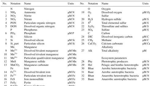
The model has 33 state variables (Table 1), including frequently measured components such as hydrogen sulfide (H2S) and phosphate (PO4), as well as rarely measured
triva-Fe(III)
O
2 H2SMn(II) S0 Mn(III) MnS Fe(II) FeS S2O3
NO2 NH4 FeS MnS Mn(IV) POM Fe(III) Fe(II) Mn(II) Mn(III)
H2S Mn(IV)
H2S
Fe(II) )I I( e F O2 O2 POM
H2S
H2S
O2 O2 H2S
O2
Mn(III)
NO2
NO3
N2
NH4 Phy
Het O2
O2 H2S
H2S NO2 S2O3 POM
NH4
S2O3 POM
Bhae
Baaeaan
B Bhan ΣOM PO4 TIC P Mn(IV) Mn(III) O2 Mn(IV) NO2 Fe(III) S0
S2O3
NO3 SO4 SO4
S2O3
S0
H2S Mn(IV) Mn(III) Fe(III) O2 NO2 NO3 OM FeS MnS Mn(II) Fe(II)
O2 DOM
O2 O2
O2 NO3
H2O
H2O
NO3 NO3
(a)
(b)
(c)
(d)
e)
(g)
CaCO3 CO2 HCO3 CO3 TIC AΣH2S ΣH2SO4P pH
f)
S0 Phy Het POM DOM Mn(III) N2 Mn(II)NO2+NH4 NO2 NO3 NH4 Fe(II) Fe(III) SO4
H2S PO4 NH4 Mn(III) Fe(III) Mn(II) Fe(II) S0
S2O3
MnO2
NO3 NO2 NH4
NO2
Mn(III)
AB [OH-] [H+]
AF
ASi
A
AΣNH3
A
ΣOM
bounded
FeS2 O2
H2S H2S
SO4 FeS FeS2 Si partSi FeS2
H2S
SO4 O2 HCO3 MnCO3 MnCO3 ΣOM M O P HCO3 M O D DOM DOM POM DOM DOM FeCO3 CH4 At Bhan
Bhae Baan Baae
Phy
Figure 1.Flow chart of biogeochemical processes represented in the Benthic RedOx Model (BROM), showing the transformation of sulfur
species(a), the ecological block(b), the transformation of nitrogen species(c), the transformation of iron species(d), the processes affecting dissolved oxygen(e), the carbonate system and alkalinity(f), and the transformation of manganese species(g).
lent manganese species Mn(III), and bacteria. We acknowl-edge that for many of these, site-specific estimates of associ-ated model parameters and initial/boundary conditions may be difficult or impossible to obtain, and may in practice re-quire some crude assumptions and approximations (e.g., uni-versal default parameter values, no-flux boundary conditions, and initial conditions from a steady annual cycle). Neverthe-less, we believe that for many applications this caveat will be acceptable given the additional process resolution and real-ism provided by BROM for important biogeochemical pro-cesses in the BBL and sediments. The equations and param-eters employed in BROM are given in Tables 2 and 3, and a flow chart is shown in Fig. 1.
2.1.2 Ecosystem and redox models
The overall goal of the ecosystem representation is to pa-rameterize the key features of OM production and de-composition, following Redfield and Richards stoichiometry (Richards, 1965). We divide all the living OM (biota) into Phy (photosynthetic biota), Het (non-microbial heterotrophic
biota), and four groups of “bacteria” which may be consid-ered to include microbial fungi. These latter are Baae (aero-bic chemoautotrophic bacteria), Baan (anaero(aero-bic chemoau-totrophic bacteria), Bhae (aerobic heterotrophic bacteria), and Bhan (anaerobic heterotrophic bacteria). OM is produced photosynthetically by Phy and chemosynthetically by bacte-ria, specifically by Baae in oxic conditions and by Baan in anoxic conditions. Growth of heterotrophic bacteria is tied to mineralization of OM, favoring Bhae in oxic conditions and Bhan in anoxic conditions. Secondary production is repre-sented by Het, which consumes phytoplankton as well as all types of bacteria and dead particulate organic matter (detri-tus, which is also explicitly modeled). The effect of suboxia and anoxia is parameterized by letting the mortality of aero-bic organisms depend on the oxygen availability.
No. Notation Name Units No. Notation Name Units
N Nitrogen O Oxygen
1 NH4 Ammonia µM N 19 O2 Dissolved oxygen µM O2
2 NO2 Nitrite µM N S Sulfur
3 NO3 Nitrate µM N 20 H2S Hydrogen sulfide µM S
4 PON Particulate organic nitrogen µM N 21 S0 Total elemental sulfur µM S
5 DON Dissolved organic nitrogen µM N 22 S2O3 Thiosulfate and sulfites µM S
P Phosphorus 23 SO4 Sulfate µM S
6 PO4 Phosphate µM P C Carbon
Si Silicon 24 DIC Dissolved inorganic carbon µM C
7 Si Dissolved silicon µM Si 25 CH4 Methane µM C
8 Si_part Particulate silicon µM Si 26 CaCO3 Calcium carbonate µM Ca
Mn Manganese Alkalinity
9 Mn2+ Dissolved bivalent manganese µM Mn 27 Alk Total alkalinity µM
10 Mn3+ Dissolved trivalent manganese µM Mn
11 Mn4+ Particulate quadrivalent manganese µM Mn Ecosystem parameters
12 MnS Manganese sulfide µM Mn 28 Phy Phototrophic producers µM N
13 MnCO3 Manganese carbonate µM Mn 29 Het Pelagic and benthic heterotrophs µM N
Fe Iron 30 Bhae Aerobic heterotrophic bacteria µM N
14 Fe2+ Dissolved bivalent iron µM Fe 31 Baae Aerobic autotrophic bacteria µM N 15 Fe3+ Particulate trivalent iron µM Fe 32 Bhan Anaerobic heterotrophic bacteria µM N
16 FeS Iron monosulfide µM Fe 33 Baan Anaerobic autotrophic bacteria µM N
17 FeS2 Pyrite µM Fe
18 FeCO3 Ferrous Carbonate µM Fe
limitation, and substrate consumption rates for heterotrophs. The redox-dependent switches are mostly based on hyper-bolic tangent functions which improve system stability com-pared with discrete switches. The nutrient limitation and het-erotrophic transfer functions are based on squared Monod laws for nutrient–biomass ratio, which also stabilizes the sys-tem compared with Michaelis–Menten and Ivlev formula-tions. Here, we describe the parameterization of carbon that was not considered in ROLM and was not described in Yaku-shev (2013).
2.1.3 Total alkalinity
Total alkalinity,AT, is a model state variable. Following the
formal definition ofAT(Dickson, 1992; Wolf-Gladrow et al.,
2007; Zeebe and Wolf-Gladrow, 2001), the following alka-linity components were considered:
AT=ATCO2+AB+ATPO4+ASi+ANH3+AH2S+ [OH−] −ASO4−AHF−AHNO3− [H+],
where the carbonate alkalinity
(ATCO2=[HCO−3]+2[CO 2−
3 ]), phosphoric alkalinity
(ATPO4=[HPO24−]+2[PO34−]−[H3PO4]), silicic alkalinity
(ASi=[H3SiO−4]), ammonia alkalinity (ANH3=[NH3]), and
hydrogen sulfide alkalinity (AH2S=[HS−]) were calculated
from the corresponding model state variables (Table 1) according to Luff et al. (2001) and Volkov (1984). The
boric alkalinity AB=[B(OH)−4] was estimated from total
dissolved boron, which in turn was calculated from salinity. [OH−] and [H+] were calculated using the ion product
of water (Millero, 1995). The hydrogen sulfate alkalinity (ASO4= [HSO−4]), hydrofluoric alkalinity (AHF= [HF]),
and nitrous acid alkalinity (AHNO3=[HNO2]) were ignored
due to their insignificant impact onAT variations in most
natural marine and freshwater systems.
Biogeochemical processes can lead to either increase or decrease of alkalinity, and alkalinity can be used as an in-dicator of specific biogeochemical processes (Soetaert et al., 2007). Organic matter production can affect alkalinity via the “nutrient-H+compensating principle” formulated by Wolf-Gladrow et al. (2007): during uptake or release of charged nutrient species, electroneutrality is maintained by consump-tion or producconsump-tion of a proton (i.e., during uptake of nitrate for photosynthesis or denitrification, or production of nitrate by nitrification).
BROM also considers the effect on alkalinity of the fol-lowing redox reactions occurring in suboxic and anoxic conditions via production or consumption of [OH−] and [H+] and changes in other “standard” alkalinity components
ATCO2andAH2S(see bold font):
4Mn2++O2+4H+→4Mn3++2H2O
2Mn3++3H2O+0.5O2→2MnO2+6H+
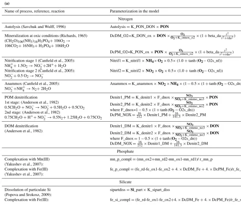
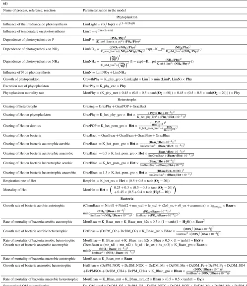
Table 2.Parameterization of the biogeochemical processes:(a)nutrients;(b)redox metals and sulfur;(c)carbon and alkalinity;(d)ecosystem processes.
(a)
Name of process, reference, reaction Parameterization in the model Nitrogen
Autolysis (Savchuk and Wulff, 1996) Autolysis=K_PON_DON×PON Mineralization at oxic conditions (Richards, 1965)
(CH2O)106(NH3)16H3PO4+106O2→
106CO2+16NH3+H3PO4+106H2O
DcDM_O2=K_DON_ox×DON× O2
O2+K_omox_o2
×(1+beta_da t2
t2+tda2)
DcPM_O2=K_PON_ox×PON× O2
O2+K_omox_o2×(1+beta_da
t2
t2+tda2)
Nitrification stage 1 (Canfield et al., 2005): NH+4+1.5O2→NO−2+2H
++H
2O
Nitrif1=K_nitrif1×NH4×O2×0.5×(1.0+tanh (O2−O2s_nf))
Nitrification stage 2 (Canfield et al., 2005): NO−2+0.5 O2→NO−3
Nitrif2=K_nitrif2×NO2×O2×0.5×(1.0+tanh (O2−O2s_nf))
Anammox (Canfield et al., 2005): NO−2+NH+4 →N2+2H2O
Anammox=K_anammox×NO2×NH4×(1−0.5×(1+tanh(O2−O2s_dn)))
POM denitrification
1st stage: (Anderson et al., 1982) 0.5CH2O+NO−3 →NO
−
2+0.5H2O+0.5CO2
2nd stage: (Anderson et al., 1982)
0.75CH2O+H++NO−2 →0.5N2+1.25H2O+0.75CO2
Denitr1_PM=K_denitr1×F_dnox× NO3
NO3+K_ommo_no3×PON Denitr2_PM=K_denitr2×F_dnox× NO2
NO2+K_ommo_no2×PON where F_dnox=1−0.5×(1+tanh(O2−O2s_dn))
DcPM_NOX= 16
212×Denitr1_PM+ 16
141.3×Denitr2_PM
DOM denitrification (Anderson et al., 1982)
Denitr1_DM=K_denitr1×F_dnox× NO3
NO3+K_ommo_no3×DON Denitr2_DM=K_denitr2×F_dnox× NO2
NO2+K_ommo_no3×DON where F_dnox=1−0.5×(1+tanh(O2−O2s_dn))
DcDM_NOX= 16
212×Denitr1_DM+ 16
141.3×Denitr2_DM
Phosphate Complexation with Mn(III)
(Yakushev et al., 2007):
mn_p_compl=(mn_ox2+mn_rd2-mn_ox1-mn_rd1)/ r_mn_p Complexation with Fe(III)
(Yakushev et al., 2007):
fe_p_compl=(fe_rd-fe_ox1-fe_ox2+4.×DcDM_Fe+4.×DcPM_Fe)/r_fe_p
Silicate Dissolution of particulate Si
(Popova and Srokosz, 2009):
sipartdiss=Si_part×K_sipart_diss
Complexation with Fe(III): fe_si_compl=(fe_rd-fe_ox1-fe_ox2+4.×DcDM_Fe+4.×DcPM_Fe)/r_fe_si
2Mn3++HS−→2Mn2++S0+H+
Mn2++HS−↔MnS+H+
Mn2++CO23−↔MnCO3
2MnCO3+O2+2H2O→2MnO2+2HCO−3 +2H
+
4Fe2++O2+10H2O→4Fe(OH)3+8H+
2Fe2++MnO2+4H2O→2Fe(OH)3+Mn2++2H+
2Fe(OH)3+HS−+5H+→2Fe2++S0+6H2O
Fe2++HS−↔FeS+H+
FeS+2.25O2+2.5H2O→Fe(OH)3+2H++SO24−
FeS2+3.5O2+H2O→Fe2++2SO24−+2H+
Fe2++CO23−↔FeCO3
NH+4 +1.5O2→NO−2 +2H++H2O
0.75CH2O+H++NO−2 →0.5N2+1.25H2O+0.75CO2
4S0+3H2O→2H2S+S2O23−+2H+
2S0+O2+H2O→S2O23−+2H
+
4S0+3NO−3 +7H2O→4SO24−+3NH+4 +2H+
S2O23−+2O2+2OH−→2SO24−+H2O
5H2S+8NO−3 +2OH−→5SO24−+4N2+6H2O
Ca2++CO23−↔CaCO3.
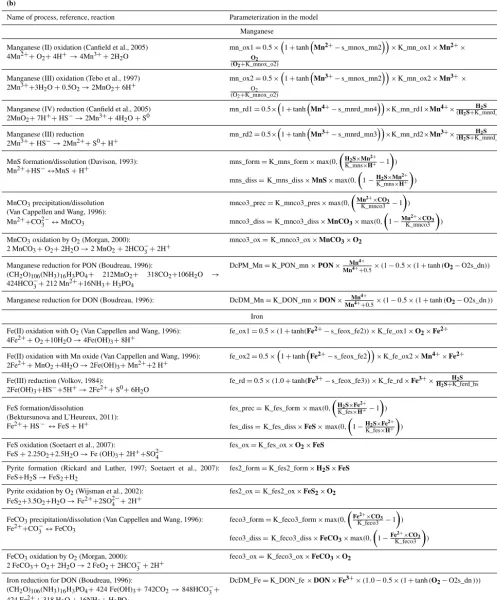
Table 2.Continued.
(b)
Name of process, reference, reaction Parameterization in the model
Manganese
Manganese (II) oxidation (Canfield et al., 2005) 4Mn2++O2+4H+→4Mn3++2H2O
mn_ox1=0.5×1+tanhMn2+−s_mnox_mn2×K_mn_ox1×Mn2+×
O2
(O2+K_mnox_o2)
Manganese (III) oxidation (Tebo et al., 1997) 2Mn3++3H
2O+0.5O2→2MnO2+6H+
mn_ox2=0.5×1+tanhMn3+−s_mnox_mn2×K_mn_ox2×Mn3+× O2
(O2+K_mnox_o2)
Manganese (IV) reduction (Canfield et al., 2005) 2MnO2+7H++HS−→2Mn3++4H2O+S0
mn_rd1=0.5×1+tanhMn4+−s_mnrd_mn4×K_mn_rd1×Mn4+× H2S
(H2S+K_mnrd_hs)
Manganese (III) reduction 2Mn3++HS−→2Mn2++S0+H+
mn_rd2=0.5×1+tanhMn3+−
s_mnrd_mn3×K_mn_rd2×Mn3+× H2S
(H2S+K_mnrd_hs)
MnS formation/dissolution (Davison, 1993): Mn2++HS−↔MnS+H+
mns_form=K_mns_form×max(0,
H2S×Mn2+ K_mns×H+−1
)
mns_diss=K_mns_diss×MnS×max(0,
1−H2S×Mn2+ K_mns×H+
)
MnCO3precipitation/dissolution
(Van Cappellen and Wang, 1996): Mn2++CO2−
3 ↔MnCO3
mnco3_prec=K_mnco3_pres×max(0,
Mn2+×
CO3 K_mnco3 −1
)
mnco3_diss=K_mnco3_diss×MnCO3×max(0,
1−Mn 2+×
CO3 K_mnco3
)
MnCO3oxidation by O2(Morgan, 2000):
2 MnCO3+O2+2H2O→2 MnO2+2HCO−3+2H
+
mnco3_ox=K_mnco3_ox×MnCO3×O2
Manganese reduction for PON (Boudreau, 1996):
(CH2O)106(NH3)16H3PO4+ 212MnO2+ 318CO2+106H2O →
424HCO−3+212 Mn2++16NH
3+H3PO4
DcPM_Mn=K_PON_mn×PON× Mn4+
Mn4+
+0.5×(1−0.5×(1+tanh(O2−O2s_dn))
Manganese reduction for DON (Boudreau, 1996): DcDM_Mn=K_DON_mn×DON× Mn4
+
Mn4++
0.5×(1−0.5×(1+tanh(O2−O2s_dn))
Iron
Fe(II) oxidation with O2(Van Cappellen and Wang, 1996):
4Fe2++O2+10H2O→4Fe(OH)3+8H+
fe_ox1=0.5×(1+tanh(Fe2+−s_feox_fe2))×K_fe_ox1×O2×Fe2+
Fe(II) oxidation with Mn oxide (Van Cappellen and Wang, 1996): 2Fe2++MnO2+4H2O→2Fe(OH)3+Mn2++2 H+
fe_ox2=0.5×
1+tanhFe2+−s_feox_fe2×K_fe_ox2×Mn4+×Fe2+
Fe(III) reduction (Volkov, 1984):
2Fe(OH)3+HS−+5H+→2Fe2++S0+6H2O
fe_rd=0.5×(1.0+tanh(Fe3+−s_feox_fe3))×K_fe_rd×Fe3+× H2S H2S+K_ferd_hs
FeS formation/dissolution
(Bektursunova and L’Heureux, 2011): Fe2++HS−↔FeS+H+
fes_prec=K_fes_form×max(0,
H2S×Fe2+ K_fes×H+−1
)
fes_diss=K_fes_diss×FeS×max(0,
1−H2S×Fe2+ K_fes×H+
)
FeS oxidation (Soetaert et al., 2007):
FeS+2.25O2+2.5H2O→Fe (OH)3+2H++SO24−
fes_ox=K_fes_ox×O2×FeS
Pyrite formation (Rickard and Luther, 1997; Soetaert et al., 2007): FeS+H2S→FeS2+H2
fes2_form=K_fes2_form×H2S×FeS
Pyrite oxidation by O2(Wijsman et al., 2002):
FeS2+3.5O2+H2O→Fe2++2SO24−+2H
+
fes2_ox=K_fes2_ox×FeS2×O2
FeCO3precipitation/dissolution (Van Cappellen and Wang, 1996):
Fe2++CO−3↔FeCO3
feco3_form=K_feco3_form×max(0,
Fe2+×
CO3 K_feco3 −1
)
feco3_diss=K_feco3_diss×FeCO3×max(0,
1−Fe 2+×
CO3 K_feco3
)
FeCO3oxidation by O2(Morgan, 2000):
2 FeCO3+O2+2H2O→2 FeO2+2HCO−3+2H
+
feco3_ox=K_feco3_ox×FeCO3×O2
Iron reduction for DON (Boudreau, 1996):
(CH2O)106(NH3)16H3PO4+424 Fe(OH)3+742CO2→848HCO−3+
424 Fe2++318 H2O+16NH3+H3PO4
DcDM_Fe=K_DON_fe×DON×Fe3+×(1.0−0.5×(1+tanh(O
2−O2s_dn)))
Iron reduction for PON (Boudreau, 1996): DcPM_Fe=K_PON_fe×PON×Fe3+×(1.0−0.5×(1+tanh(O
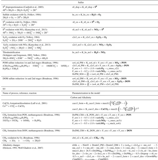
Table 2.Continued.
Sulfur
S0disproportionation (Canfield et al., 2005):
4S0+3H2O→2H2S+S2O23−+2H
+
s0_disp=K_s0_disp×S0
Sulfide oxidation with O2(Volkov, 1984):
2H2S+O2→2S0+2H2O
hs_ox=K_hs_ox×H2S×O2
S0oxidation with O2(Volkov, 1984):
2S0+O2+H2O→S2O23−+2H
+ s0_ox
=K_s0_ox×S0×O2
S0oxidation with NO3(Kamyshny et al., 2013):
4S0+3NO−3+7H2O→4SO24−+3NH
+
4+2H
+
s0_no3=K_s0_no3×NO3×S0
S2O3oxidation with O2(Volkov, 1984):
S2O23−+2O2+2OH−→2SO24−+H2O
s2o3_ox=K_s2o3_ox×S2O3×O2
S2O3oxidation with NO3(Kamyshny et al., 2013):
S2O23−+NO
−
3+2H2O→2SO24−+NH
+
4
s2o3_no3=K_s2o3_no3×NO3×S2O3
Thiodenitrification
(Schippers and Jorgensen, 2002; Volkov, 1984): 5H2S+8NO−3+2OH
−→
5SO24−+4N2+6H2O
hs_no3=K_hs_no3×H2S×NO3
POM sulfate reduction 1st and 2nd stages (Boudreau, 1996): (CH2O)106(NH3)16H3PO4+ 53SO24−→ 106HCO
−
3+ 16NH3+
H3PO4+53H2S
so4_rd_PM=K_so4_rd×F_sox×F_snx×SO4×PON
s2o3_rd_PM=K_s2o3_rd×F_sox×F_snx×S2O3×PON
F_sox=1−0.5×(1.0+tanh(O2−s_omso_o2))
F_snx=1−0.5×(1.0+tanh(NO3−s_omso_no3))
DcPM_SO4=16
53×(so4_rd_PM+s2o3_rd_PM)
DOM sulfate reduction 1st and 2nd stages (Boudreau, 1996): so4_rd_DM=K_so4_rd×F_sox×F_snx×SO4×DON
s2o3_rd_DM=K_s2o3_rd×F_sox×F_snx×S2O3×DON
DcDM_SO4=16
53×(so4_rd_PM+s2o3_rd_PM)
(c)
Name of process, reference, reaction Parameterization in the model
Carbon and Alkalinity
CaCO3formation/dissolution (Luff et al., 2001):
Ca2++CO23↔CaCO3
caco3_form=K_caco3_form×max(0,
Ca2+×
CO3 K_caco3 −1
)
caco3_diss=K_caco3_diss×CaCO3×max(0,
1−Ca2
+×
CO3 K_caco3
)4.5
CH4formation from PON, methanogenesis (Boudreau, 1996):
(CH2O)106(NH3)16H3PO4 →
53CO2+53CH4 +16NH3 +H3PO4
DcPM_CH4=K_PON_ch4×F_sox×F_snx×F_ssx×PON F_sox=1−0.5×(1.0+tanh(O2−s_omso_o2))
F_snx=1−0.5×(1.0+tanh(NO3−s_omso_no3))
F_ssx=1−0.5×(1.0+tanh(SO4−s_omch_so4))
CH4formation from DON, methanogenesis (Boudreau, 1996) DcDM_CH4=K_DON_ch4×F_sox×F_snx×F_ssx×DON
CH4oxidation by O2(Boudreau, 1996):
CH4 +2O2 + →CO2 +2H2O
ch4_o2=K_ch4_o2×CH4×O2
Alkalinity changes
(Dickson, 1992; Wolf-Gladrow et al., 2007)
dAlk= −Nitrif1+Denitr2_PM+Denitr2_DM+2×(so4rd+s2o3rd)+mn_ox1 −3×
mn_ox2+3×mn_rd1−mn_rd2−2×mns_form+2×mns_diss−2×mnco3_form+2×
mnco3_diss+26.5×(DcDMMn+DcPMMn)−2×fe_ox1−fe_ox2+2×fe_rd−fes_form+
fes_diss−2×fes_ox−2×fes2_ox+53×(DcDMFe+DcPMFe)−0.5×Disprop+s0_ox−
0.5×s_no3−s2o3_ox−0.4×hs_no3−2×caco3_form+2×caco3_diss+GrowthPhy×
LimNO3 LimN
−GrowthPhy×LimNH4 LimN
2.1.4 Carbonate system
Equilibration of the carbonate system was considered as a fast process occurring within seconds (Zeebe and Wolf-Gladrow, 2001). Accordingly, the equilibrium solution was calculated at every time step using an iterative procedure. The carbonate system was described using standard ap-proaches (Lewis and Wallace, 1998; Munhoven, 2013; Roy
Table 2.Continued.
(d)
Name of process, reference, reaction Parameterization in the model
Phytoplankton
Influence of the irradiance on photosynthesis LimLight=(Iz
Iopt)×e(1−Iz/Iopt)
Influence of temperature on photosynthesis LimT=e(bm×t−cm)
Dependence of photosynthesis on P LimP= (PO4/Phy)2
(K_po4_lim×r_n_p)2+(PO 4/Phy)2
Dependence of photosynthesis on NO3 LimNO3= ((NO3+NO2)/Phy)
2
K_nox_lim2+((NO
3+NO2)/Phy)2
exp(−K__psi (NH4/Phy)2
K_nh4_lim2+(NH 4/Phy)2
)
Dependence of photosynthesis on NH4 LimNH4=
NH4
Phy
2
K_nh4_lim2+NH4
Phy
2(1−exp(−K__psi
(NH4/Phy)2
K_nh4_lim2+(NH 4/Phy)2
))
Influence of N on photosynthesis LimN=LimNO3+LimNH4
Growth of phytoplankton GrowthPhy=K_phy_gro×LimLight×LimT×min(LimP,LimN)×Phy Excretion rate of phytoplankton ExcrPhy=K_phy_exc×Phy
Phytoplankton mortality rate MortPhy=(K_phy_mrt+0.45×(0.5−0.5×tanh(O2−60) )+0.45×(0.5−0.5×tanh(O2−20) ) )×Phy
Heterotrophs
Grazing of heterotrophs Grazing=GrazPhy+GrazPOP+GrazBact
Grazing of Het on phytoplankton GrazPhy=K_het_phy_gro×Het× (Phy/(Het+10 −4))2
K_het_phy_lim2+(Phy/(Het+10−4))2
Grazing of Het on detritus GrazPOP=K_het_pom_gro×Het× (
PON Het+10−4)2
K_het_pom_lim2+( PON Het+10−4)2 Grazing of Het on bacteria GrazBact=GrazBaae+GrazBaan+GrazBhae+GrazBhan
Grazing of Het on bacteria autotrophic aerobic GrazBaae =K_het_pom_gro×Het× (Baae/(Het+10 −4))2
limGrazBac2+(Baae/(Het+10−4))2
Grazing of Het on bacteria autotrophic anaerobic GrazBaan=0.5×K_het_pom_gro×Het× (Baan/(Het+10 −4))2
limGrazBac2+
(Baan/(Het+10−4
))2
Grazing of Het on bacteria heterotrophic aerobic GrazBhae=K_het_pom_gro×Het× (Bhae/(Het+10 −4))2
limGrazBac2+(Bhae/(Het+10−4)2
Grazing of Het on bacteria heterotrophic anaerobic GrazBhan=1.3×K_het_pom_gro×Het× (Bhan/Het+0.0001)2
limGrazBac2+(Bhan/Het+10−4)2 Respiration rate of Het RespHet=K_het_res×Het×(0.5+0.5×tanh(O2−20))
Mortality of Het MortHet=Het×
0
.25+0.3×(0.5−0.5×tanh(O2−20)) +0.45×(0.5+0.4×tanh(H2S−10))
Bacteria
Growth rate of bacteria aerobic autotrophic (ChemBaae=Nitrif1+Nitrif2+mn_ox1+fe_ox1+s2o3_ox+s0_ox+anammox)×kBaaegro×Baae×
min( (NH4/(Baae+10 −42
limBaae2+(NH
4/(Baae+10−4))2
, (PO4/(Baae+10−4))2
limBaae2+(PO
4/(Baae+10−4))2
)
Rate of mortality of bacteria aerobic autotrophic MortBaae=K_Baae_mrt+K_Baae_mrt_h2s×0.5×(1−tanh(1−H2S))×Baae2
Growth rate of bacteria aerobic heterotrophic HetBhae=(DcPM_O2+DcDM_O2)×K_Bhae_gro×Bhae× DON
Bhae+10−42
limBhae2+DON
Bhae+10−42
Rate of mortality of bacteria aerobic heterotrophic MortBhae=K_Bhae_mrt+K_Bhae_mrt_h2s×Bhae×0.5×(1−tanh(1−H2S))
Growth rate of bacteria anaerobic autotrophic ChemBaan=(mn_rd1+mn_rd2+fe_rd+hs_ox+hs_no3)×K_Baan_gro×Baan×
min?( (NH4/(Baan+10 −4))2
limBaan2+(NH4/(Baan+10−4))2 Rate of mortality of bacteria anaerobic autotrophic MortBaan=K_Baan_mrt×Baan
Growth rate of bacteria anaerobic heterotrophic HetBhan=(DcPM_NOX+DcDM_NOX+DcDM_Mn+DcPM_Mn+DcDM_Fe+DcPM_Fe+DcDM_SO4
+DcPMSO4+DcDM_CH4+DcPM_CH4)×K_Bhan_gro×Bhan× (DON/(Bhan+10 −4))2
limBhan2+(DON/(Bhan+10−4))2 Rate of mortality of bacteria anaerobic heterotrophic MortBhan=K_Bhan_mrt+K_Bhan_mrt_o2×Bhan×(0.5+0.5×tanh(1−O2))
Summarized OM mineralization Dc_OM_total=DcDM_O2+DcPM_O2+DcPM_NOX+DcDM_NOX+DcDM_Mn+DcPM_Mn+DcDM_Fe
water was calculated according to Millero (1995). Total scale pH was calculated using the Newton–Raphson method with the modifications proposed in Munhoven (2013). Precipita-tion and dissoluPrecipita-tion of calcium carbonate were modeled fol-lowing the approach of Luff et al. (2001) (Table 2).
2.1.5 Physical environment
BROM-biogeochemistry can be coupled online with vari-ous hydrodynamic models using FABM, but this may quire extensive adaptation of the hydrodynamic model to re-solve the BBL and upper sediments. We have therefore devel-oped a simple 1-D offline transport-reaction model, BROM-transport, whose model domain spans the water column, BBL, and upper layers of the sediments, with enhanced stial resolution in the BBL and sediments. All options and pa-rameter values for BROM-transport are specified in a run-time input file brom.yaml. A step-by-step guide to running BROM-transport is provided in Appendix A.
2.1.6 BROM-transport model formulation
The time–space evolution of state variables in BROM-transport is described by a system of 1-D BROM-transport-reaction equations in Cartesian coordinates. In the water column, the dynamics are
∂Cˆi ∂t =
∂ ∂zD
∂Cˆi ∂z −
∂ ∂zvi
ˆ Ci+εh
ˆ C0i− ˆCi
+Tbirr(i)+Ri, (1)
whereCˆi is the concentration in units [mmol m−3total
vol-ume] of the ith state variable, D(z, t )is the vertical diffu-sivity,vi is the settling or sinking velocity,εh(z, t )is a rate
of horizontal mixing with an external concentrationCˆ0i(z, t )
(or alternatively, a restoring rate to a climatological concen-tration),Tbirr(i)is a tendency due to bioirrigation (only
non-zero for dissolved substances in the bottom layer of the wa-ter column; see below), andRi is the combined sources
mi-nus sinks (in this study provided by BROM-biogeochemistry, but in principle any biogeochemical model in FABM could be used). Values for D, εh, Cˆ0i, and other forcings used
by Ri are configured at runtime through input files (see
Sect. 2.2.7). Sinking velocitiesvi are non-zero only for
par-ticulate (non-dissolved) variables and are determined at each time step by the biogeochemical module (through FABM). BROM-biogeochemistry assumes constant sinking velocities for phytoplankton, zooplankton, bacteria, detritus, and inor-ganic particles (Table 3e).
In the sediments, dissolved substances or solutes obey the dynamics
ϕ∂Ci ∂t =
∂ ∂zϕDC
∂Ci ∂z −
∂
∂zϕuCi+TbirrC(i)+Ri, (2)
whereϕis the porosity (assumed constant in time),DCis the
total solute diffusivity,uis the solute burial velocity, andCi
is the porewater concentration in units [mmol m−3 porewa-ter]. Particulate substances become part of the solid matrix in the sediments. These obey
(1−ϕ)∂Bi ∂t =
∂
∂z(1−ϕ) DB ∂Bi
∂z
− ∂
∂z(1−ϕ) wBi+Ri, (3)
whereDB is the particulate (bioturbation) diffusivity,w is
the particulate burial velocity, andBi is the particulate
con-centration in units [mmol m−3total solids].
The porosityϕ(z)in Eqs. (2) and (3) is prescribed as an exponential decay, following Soetaert et al. (1996):
ϕ=ϕ∞+(ϕ0−ϕ∞) e
−(z−zSWI)
δ , (4)
whereϕ∞ is the deep (compacted) porosity,ϕ0is the
sedi-ment surface porosity,zSWIis the depth of the SWI, andδis
a decay scale defining the rate of compaction.
Diffusion within the sediments is assumed to be strictly “intraphase” (Boudreau, 1997), hence the Fickian gradients in Eqs. (2) and (3) are formed using the concentration per unit volume porewater for solutes and per unit volume total solids for particulates. The total solute diffusivityDC=Dm+DB,
where Dm is the apparent molecular/ionic diffusivity and DBis the bioturbation diffusivity due to animal movement
and ingestion/excretion. The apparent molecular diffusiv-ityDm(z)=θ−2D0µµ0
sw is derived from the infinite-dilution
molecular diffusivity D0 (an input parameter) assuming a
constant relative dynamic viscosity µ0
µsw (default value 0.94,
cf. Boudreau, 1997, Table 4.10) and a tortuosity parameter-ized asθ2=1−2 lnϕfrom Boudreau (1997, Eq. 4.120). The bioturbation diffusivityDB(z, t )is modeled as a Michaelis–
Menten function of the dissolved oxygen concentration in the bottom layer of the water column:
DB(z, t )=DBmax(z)
O2s
O2s+KO2s
, (5)
whereDBmax(z)is a constant over a fixed mixed layer depth
in the surface sediments, then decays to zero with increasing depth, andKO2s is a half-saturation constant. The rationale
for Eq. (5) is that the benthic animals that cause bioturba-tion require a source of oxygen at the sediment surface for respiration.
Diffusion between the sediments and water column, i.e., across the SWI, raises a subtle issue in regard to particulates. Here, any diffusive flux cannot be strictly intraphase, because particulates are modeled as [mmol m−3 total solids] in the
sulfur;(c)carbon;(d)ecosystem parameters;(e)sinking.
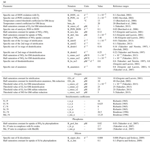
(a)
Parameter Notation Units Value Reference ranges
Nitrogen
Specific rate of DON oxidation with O2 K_DON_ ox d−1 1×10⁻² 0.1 (Savchuk, 2002) Specific rate of PON oxidation with O2 K_PON_ ox d−1 2×10⁻³ 0.002 (Savchuk, 2002) Temperature control threshold coefficient for OM decay Tda ◦C 13 13 (Burchard et al., 2006) Temperature control coefficient for OM decay beta_da – 20 20 (Burchard et al., 2006) Half-saturation constant of O2for OM mineralization K_omox_o2 µM 1 1 (Yakushev, 2013) Specific rate of autolysis, PON to DON K_PON_DON d−1 0.1 0.02 (Burchard et al., 2006) Half-saturation constant for uptake of NO3+NO2 K_nox_lim µM 0.12 0.5 (Gregoire and Lacroix, 2001) Half-saturation constant for uptake of NH4 K_nh4_ lim µM 2×10⁻² 0.2 (Gregoire and Lacroix, 2001) Strength of NH4inhibition of NO3uptake constant K_psi – 1.46 1.46 (Gregoire and Lacroix, 2001) Specific rate of the 1st stage of nitrification K_nitrif1 d−1 1×10⁻² 0.01 (Yakushev, 2013)
Specific rate of the 2nd stage of nitrification K_nitrif2 d−1 0.1 0.1 (Yakushev, 2013)
Specific rate of 1st stage of denitrification K_denitr1 d−1 0.16 0.16 (Yakushev and Neretin, 1997), 0.5 (Savchuk, 2002)
Specific rate of 2nd stage of denitrification K_denitr2 d−1 0.25 0.22 (Yakushev and Neretin, 1997) Half-saturation of NO3for OM denitrification k_omno_no3 µM N 1×10⁻³ 1×10⁻³(Yakushev, 2013) Half-saturation of NO2for OM denitrification k_omno_no2 µM N 1×10⁻³ 1×10⁻³(Yakushev, 2013)
Specific rate of thiodenitrification K_hs_no3 µM−1d−1 0.8 0.8 (Yakushev and Neretin, 1997), 0.015 (Gregoire and Lacroix, 2001)
Specific rate of anammox K_anammox d−1 0.8 0.8 (Gregoire and Lacroix, 2001), 0.03
(Yakushev et al., 2007) Oxygen
Half-saturation constant for nitrification O2s_nf µM 5.0 10 (Gregoire and Lacroix, 2001) Half-saturation constant for denitrification anammox, Mn reduction O2s_dn µM 10 40 (Savchuk, 2002)
Threshold value of O2for OM mineralization s_omox_o2 µM 1×10⁻² 1×10⁻²(Yakushev, 2013)
Threshold value of O2for OM denitrification s_omno_o2 µM 25 25 (Yakushev, 2013)
Threshold value of O2for OM sulfate reduction s_omso_o2 µM 25 25 (Yakushev, 2013) Threshold value of NO for OM sulfate reduction s_omso_ no3 µM 5 5 (Yakushev, 2013)
Stoichiometric coefficients
N/P r_n_p – 16 Richards (1965)
O/N r_o_n – 6.625 Richards (1965)
C/N r_c_n – 8 Richards (1965)
Si/N r_si_n – 1 Richards (1965)
Fe/N r_fe_n – 26.5 Boudreau (1996)
Mn/N r_mn_n – 13.25 Boudreau (1996)
Phosphorus
Half-saturation constant for uptake of PO4by phytoplankton K_po4_lim µM 0.02 0.01 (Yakushev et al., 2007)
Fe/P ratio in complexes with Fe oxides r_fe_p – 2.7 (Yakushev et al., 2007)
Mn/P ratio in complexes with Mn(III) r_mn_p – 0.67 (Yakushev et al., 2007)
Silicon
Specific rate of Si dissolution K_sipart_diss d−1 0.008 0.008 (Popova and Srokosz, 2009) Half-saturation constant for uptake of Si by phytoplankton K_si_lim – 0.1 0.1 (Popova and Srokosz, 2009)
Fe/P ratio in complexes with Fe oxides r_fe_si – 2.7 2.7 (Yakushev et al., 2007)
model. BROM-transport therefore offers two approaches. In the first approach, the bioturbation diffusivity is set to zero on the SWI, so that only solutes can diffuse across the SWI by molecular diffusion. Since the present version of BROM-transport does not parameterize resuspension through the SWI due to fluid turbulence, the SWI thus becomes a one-way street for particulate matter, whose components can only reenter the water column after dissolution. In the second ap-proach, the bioturbation diffusivity is given by Eq. (5) on the SWI, but the bioturbation flux is interphase, mixing
concen-trations in units [mmol m−3 total volume] for both solutes and particulates. This approach is appropriate if bioturbation can be assumed to exchange fluff and sediment, or if it con-tributes significantly to particulate resuspension.
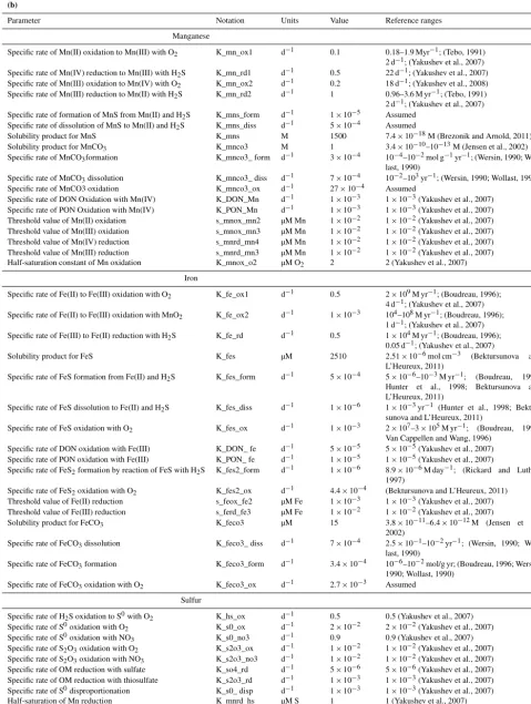
Table 3.Continued.
(b)
Parameter Notation Units Value Reference ranges
Manganese
Specific rate of Mn(II) oxidation to Mn(III) with O2 K_mn_ox1 d−1 0.1 0.18–1.9 Myr−1; (Tebo, 1991)
2 d−1; (Yakushev et al., 2007)
Specific rate of Mn(IV) reduction to Mn(III) with H2S K_mn_rd1 d−1 0.5 22 d−1; (Yakushev et al., 2007)
Specific rate of Mn(III) oxidation to Mn(IV) with O2 K_mn_ox2 d−1 0.2 18 d−1; (Yakushev et al., 2008)
Specific rate of Mn(III) reduction to Mn(II) with H2S K_mn_rd2 d−1 1 0.96–3.6 M yr−1; (Tebo, 1991)
2 d−1; (Yakushev et al., 2007) Specific rate of formation of MnS from Mn(II) and H2S K_mns_form d−1 1×10⁻⁵ Assumed
Specific rate of dissolution of MnS to Mn(II) and H2S K_mns_diss d−1 5×10⁻⁴ Assumed
Solubility product for MnS K_mns M 1500 7.4×10⁻¹⁸M (Brezonik and Arnold, 2011)
Solubility product for MnCO3 K_mnco3 M 1 3.4×10⁻¹⁰–10−13M (Jensen et al., 2002)
Specific rate of MnCO3formation K_mnco3_ form d−1 3×10⁻⁴ 10−4–10−2mol g−1yr−1; (Wersin, 1990;
Wol-last, 1990)
Specific rate of MnCO3dissolution K_mnco3_ diss d−1 7×10⁻⁴ 10−2–103yr−1; (Wersin, 1990; Wollast, 1990)
Specific rate of MnCO3 oxidation K_mnco3_ox d−1 27×10−4 Assumed
Specific rate of DON Oxidation with Mn(IV) K_DON_Mn d−1 1×10⁻³ 1×10⁻³(Yakushev et al., 2007) Specific rate of PON Oxidation with Mn(IV) K_PON_Mn d−1 1×10⁻³ 1×10⁻³(Yakushev et al., 2007) Threshold value of Mn(II) oxidation s_mnox_mn2 µM Mn 1×10⁻² 1×10⁻²(Yakushev et al., 2007) Threshold value of Mn(III) oxidation s_mnox_mn3 µM Mn 1×10⁻² 1×10⁻²(Yakushev et al., 2007) Threshold value of Mn(IV) reduction s_mnrd_mn4 µM Mn 1×10⁻² 1×10⁻²(Yakushev et al., 2007) Threshold value of Mn(III) reduction s_mnrd_mn3 µM Mn 1×10⁻² 1×10⁻²(Yakushev et al., 2007) Half-saturation constant of Mn oxidation K_mnox_o2 µM O2 2 2 (Yakushev et al., 2007)
Iron
Specific rate of Fe(II) to Fe(III) oxidation with O2 K_fe_ox1 d−1 0.5 2×10⁹M yr−1; (Boudreau, 1996);
4 d−1; (Yakushev et al., 2007) Specific rate of Fe(II) to Fe(III) oxidation with MnO2 K_fe_ox2 d−1 1×10⁻³ 104–108M yr−1; (Boudreau, 1996);
1 d−1; (Yakushev et al., 2007) Specific rate of Fe(III) to Fe(II) reduction with H2S K_fe_rd d−1 0.5 1×10⁴M yr−1; (Boudreau, 1996);
0.05 d−1; (Yakushev et al., 2007)
Solubility product for FeS K_fes µM 2510 2.51×10⁻⁶mol cm−3 (Bektursunova and
L’Heureux, 2011)
Specific rate of FeS formation from Fe(II) and H2S K_fes_form d−1 5×10⁻⁴ 5×10⁻⁶–10−3M yr−1; (Boudreau, 1996;
Hunter et al., 1998; Bektursunova and L’Heureux, 2011)
Specific rate of FeS dissolution to Fe(II) and H2S K_fes_diss d−1 1×10⁻⁶ 1×10⁻³yr−1 (Hunter et al., 1998;
Bektur-sunova and L’Heureux, 2011)
Specific rate of FeS oxidation with O2 K_fes_ox d−1 1×10⁻³ 2×10⁷–3×10⁵M yr−1; (Boudreau, 1996;
Van Cappellen and Wang, 1996) Specific rate of DON oxidation with Fe(III) K_DON_ fe d−1 5×10⁻⁵ 5×10⁻⁵(Yakushev et al., 2007) Specific rate of PON oxidation with Fe(III) K_PON_ fe d−1 1×10⁻⁵ 1×10⁻⁵(Yakushev et al., 2007)
Specific rate of FeS2formation by reaction of FeS with H2S K_fes2_form d−1 1×10⁻⁶ 8.9×10⁻⁶M day−1; (Rickard and Luther,
1997)
Specific rate of FeS2oxidation with O2 K_fes2_ox d−1 4.4×10⁻⁴ (Bektursunova and L’Heureux, 2011)
Threshold value of Fe(II) reduction s_feox_fe2 µM Fe 1×10⁻³ 1×10⁻³(Yakushev et al., 2007)
Threshold value of Fe(III) reduction s_ferd_fe3 µM Fe 1×10⁻² 1×10⁻²(Yakushev et al., 2007)
Solubility product for FeCO3 K_feco3 µM 15 3.8×10⁻¹¹–6.4×10⁻¹²M (Jensen et al.,
2002)
Specific rate of FeCO3dissolution K_feco3_ diss d−1 7×10⁻⁴ 2.5×10⁻¹–10−2yr−1; (Wersin, 1990;
Wol-last, 1990)
Specific rate of FeCO3formation K_feco3_form d−1 3.4×10⁻⁴ 10−6–10−2mol/g yr; (Boudreau, 1996; Wersin,
1990; Wollast, 1990) Specific rate of FeCO3oxidation with O2 K_feco3_ox d−1 2.7×10⁻³ Assumed
Sulfur
Specific rate of H2S oxidation to S0with O2 K_hs_ox d−1 0.5 0.5 (Yakushev et al., 2007)
Specific rate of S0oxidation with O
2 K_s0_ox d−1 2×10⁻² 2×10⁻²(Yakushev et al., 2007)
Specific rate of S0oxidation with NO
3 K_s0_no3 d−1 0.9 0.9 (Yakushev et al., 2007)
Specific rate of S2O3oxidation with O2 K_s2o3_ox d−1 1×10⁻² 1×10⁻²(Yakushev et al., 2007)
Specific rate of S2O3oxidation with NO3 K_s2o3_no3 d−1 1×10⁻² 1×10⁻²(Yakushev et al., 2007)
Specific rate of OM reduction with sulfate K_so4_rd d−1 5×10⁻⁶ 5×10⁻⁶(Yakushev et al., 2007)
Specific rate of OM reduction with thiosulfate K_s2o3_rd d−1 1×10⁻³ 1×10⁻³(Yakushev et al., 2007)
Specific rate of S0disproportionation K_s0_ disp d−1 1×10⁻³ 1×10⁻³(Yakushev et al., 2007)
Half-saturation of Mn reduction K_mnrd_hs µM S 1 1 (Yakushev et al., 2007)
Table 3.Continued.
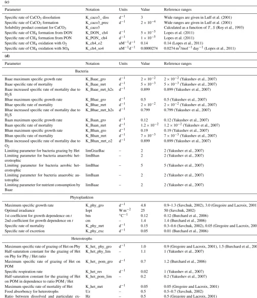
(c)
Parameter Notation Units Value Reference ranges
Specific rate of CaCO3dissolution K_caco3_ diss d−1 3 Wide ranges are given in Luff et al. (2001) Specific rate of CaCO3formation K_caco3_prec d−1 2×10⁻⁴ Wide ranges are given in Luff et al. (2001) Solubility product constant for CaCO3 K_caco3 Calculated as a function ofT,S(Roy et al., 1993) Specific rate of CH4formation from DON K_DON_ ch4 d−1 5×10⁻⁵ Lopes et al. (2011)
Specific rate of CH4formation from PON K_PON_ ch4 d−1 1×10⁻⁵ Lopes et al. (2011) Specific rate of CH4oxidation with O2 K_ch4_o2 uM−1d−1 0.14 0.14 (Lopes et al., 2011)
Specific rate of CH4oxidation with SO4 K_ch4_so4 uM−1d−1 0.0000274 0.0274 m3/mol−1day−1(Lopes et al., 2011) (d)
Parameter Notation Units Value Reference ranges
Bacteria
Baae maximum specific growth rate K_Baae_gro d−1 2×10⁻² 2×10⁻²(Yakushev et al., 2007) Baae specific rate of mortality K_Baae_mrt d−1 5×10⁻³ 5×10⁻³(Yakushev et al., 2007) Baae increased specific rate of mortality due to
H2S
K_Baae_mrt_h2s d−1 0.899 0.899 (Yakushev et al., 2007) Bhae maximum specific growth rate K_Bhae_gro d−1 0.5 0.5 (Yakushev et al., 2007) Bhae specific rate of mortality K_Bhae_mrt d−1 2×10⁻² 2×10⁻²(Yakushev et al., 2007) Bhae increased specific rate of mortality due to
H2S
K_Bhae_mrt_h2s d−1 0.799 0.799 (Yakushev et al., 2007) Baan maximum specific growth rate K_Baan_gro d−1 0.12 0.12 (Yakushev et al., 2007) Baan specific rate of mortality K_Baan_mrt d−1 1.2×10⁻² 1.2×10⁻²(Yakushev et al., 2007) Bhan maximum specific growth rate K_Bhan_gro d−1 0.19 0.19 (Yakushev et al., 2007) Bhan specific rate of mortality K_Bhan_mrt d−1 7×10⁻³ 7×10⁻³(Yakushev et al., 2007) Bhan increased specific rate of mortality due to
O2
K_Bhan_mrt_o2 d−1 0.899 0.899 (Yakushev et al., 2007) Limiting parameter for bacteria grazing by Het limGrazBac – 2 2 (Yakushev et al., 2007) Limiting parameter for bacteria anaerobic
het-erotrophic
limBhan – 2 2 (Yakushev et al., 2007)
Limiting parameter for bacteria aerobic het-erotrophic
limBhae – 5 5 (Yakushev et al., 2007)
Limiting parameter for bacteria anaerobic au-totrophic
limBaan – 2 2 (Yakushev et al., 2007)
Limiting parameter for nutrient consumption by Baae
limBaae – 2 2 (Yakushev et al., 2007)
Phytoplankton
Maximum specific growth rate K_phy_gro d−1 4.8 0.9–1.3 (Savchuk, 2002), 3.0 (Gregoire and Lacroix, 2001)
Optimal irradiance Iopt W m−2 25 50 (Savchuk, 2002)
1st coefficient for growth dependence ont bm ◦C−1 0.12 0.12 (Burchard et al., 2006) 2nd coefficient for growth dependence ont cm – 1.4 1.4 (Burchard et al., 2006)
Specific rate of mortality K_phy_mrt d−1 0.15 0.3–0.6 (Savchuk, 2002), 0.05 (Gregoire and Lacroix, 2001)
Specific rate of excretion K_phy_exc d−1 0.05 0.01 (Burchard et al., 2006)
Heterotrophs
Maximum specific rate of grazing of Het on Phy K_het_ phy_gro d−1 1.0 0.9 (Gregoire and Lacroix, 2001), 1.5 (Burchard et al., 2006) Half-saturation constant for the grazing of Het
on Phy for Phy/Het ratio
K_het_phy_lim – 1.1 1 (Yakushev et al., 2007) Maximum specific rate of grazing of Het on
POM
K_het_ pom_gro d−1 0.7 1.2 (Burchard et al., 2006)
Specific respiration rate K_het_res d−1 0.02 1 (Yakushev et al., 2007)
Half-saturation constant for the grazing of Het on POM in dependence to ratio POM/Het
K_het_pom_lim – 0.2 0.2 (Yakushev et al., 2007) Maximum specific rate of mortality of Het K_het_mrt d−1 0.05 0.05 (Gregoire and Lacroix, 2001)
Food absorbency for heterotrophs Uz – 0.5 0.5–0.7 (Savchuk, 2002)
Ratio between dissolved and particulate ex-cretes of heterotrophs
Table 3.Continued.
(e)
Parameter Notation Units Value Reference ranges
Rate of sinking of Phy Vphy m d−1 1 0.1–0.5 (Savchuk, 2002)
Rate of sinking of Het Vhet m d−1 1 1 (Yakushev et al., 2007)
Rate of sinking of bacteria (Bhae, Baae, Bhan, Baan) Vbact m d−1 0.4 0.5 (Yakushev et al., 2007)
Rate of sinking of detritus (PON) Vsed m d−1 6 0.4 (Savchuk, 2002),
1–370 (Alldredge and Gotschalk, 1988) Rate of sinking of inorganic particles (Fe and Mn hydroxides, carbonates) Vm m d−1 8 6–18 (Yakushev et al., 2007)
Table 4. Rates of biogeochemical production/consumption of the model compartments:(a)nutrients and oxygen;(b)Redox metals and
sulfur;(c)carbon and alkalinity;(d)ecosystem parameters.
(a)
Parameter Rate
O2 R O2=(GrowthPhy−RespHet−DcDM_O2−DcPM_O2)×r_o_n−0.25×mn_ox1−0.25×mn_ox2−0.25×fe_ox1−
0.5×hs_ox−0.5×s0_ox 0.5×s2o3_ox−0.5×mns_ox−1.5×Nitrif1−0.5×Nitrif2−2.25×fes_ox−3.5×fes2_ox 0.5×
mnco3_ox+feco3_ox−2×ch4_o2
Particulate organic nitrogen (PON) R PON=MortBaae+MortBaan+MortBhae+MortBhan+MortPhy+MortHet+Grazing×(1−Uz)×(1−Hz)−GrazPOP) −autolysis−DcPM_O2−DcPM_NOX−DcPM_SO4−DcPM_Mn−DcPM_Fe−0.5×DcPM_CH4
Dissolved organic nitrogen (DON) R DON=autolysis−DcDM_O2−DcDM_NOX−DcDM_SO4−DcDM_Mn−DcDM_Fe−0.5×DcPM_CH4−HetBhae−
HetBhan+ExcrPhy+Grazing×(1−Uz)×Hz
NH4 R NH4= Dc_OM_total−Nitrif1−anammox+0.75×s0_ox+s2o3_ox−ChemBaae−ChemBaan+RespHet−GrowthPhy× LimNH4
LimN
NO2 R NO2=Nitrif1−Nitrif2+Denitr1−Denitr2−anammox−GrowthPhy×LimNO3LimN × NO2 NO2+NO3+10−5
NO3 R NO3=Nitrif2−Denitr1−1.6×hs_no3−0.75 s0_ox−s2o3_ox−GrowthPhy×
LimNO
3
LimN
× NO3+10−5 NO2+NO3+10−5
PO4 R PO4=GrowthPhy+RespHet+Dc__OM__totalr_n_p −ChemBaae−ChemBaan+fe__p__compl+mn__p__compl
Si R Si=(ExcrPhy-GrowthPhy)×r_si_n+fe_si_compl
Si particulate R Si part= −K_sipart_diss×Sipart+(MortPhy+GrazPhy)×r_si_n)
(b)
Parameter Rate
Mn(II) R Mn2=mn_rd2−mn_ox1+mns_diss−mns_form−mnco3_form+mnco3_diss+0.5×fe_ox2+(DcDM_Mn+DcPM_Mn) ×r_mn_n
Mn(III) R Mn3=mn_ox1−mn_ox2+mn_rd1 mn_rd2
Mn(IV) RMn4=mn_ox2−mn_rd1−0.5×fe_ox2+mnco3_ox−(DcDM_Mn+DcPM_Mn)×r_mn_n
MnS R MnS=mns_form−mns_diss
MnCO3 R MnCO3=mnco3_form−mnco3_diss−mnco3_ox
Fe(II) R Fe2=fe_rd−fes_form−fe_ox1−fe_ox2+fes_diss−feco3_form+feco3_diss+fes2_ox+4×r_fe_n× (DcDM_Fe+DcPM_Fe)
Fe(III) R Fe3=fe_ox1+fe_ox2−fe_rd+fes_ox+feco3_ox−4×r_fe_n×(DcDM_Fe+DcPM_Fe)
FeS R FeS=fes_form−fes_diss−fes_ox−fes2_form
FeS2 R FeS2=fes2_form−fes2_ox
FeCO3 R FeCO3=feco3_form−feco3_diss−feco3_ox
H2S R H2S=0.5×s0_disp−hs_no3+s2o3_rd−fes2_form−0.5×mn_rd1−0.5×mn_rd2−0.5×fe_rd−hs_ox+fes_diss−fes_form+
mns_diss−mns_form
S0 R S0=hs_ox+0.5×mn_rd1+0.5×mn_rd2+0.5×fe_rd−s0_ox−s0_disp−s_no3 S2O3 R S2O3=0.5×s0_ox−s2o3_ox+0.25×s0_disp+0.5×so4_rd−0.5×s2o3_rd−s2o3_no
SO4 RSO4=hs_no3−so4_rd+0.5×s2o3_ox+s_no3+2×s2o3_no3+fes_ox+2×fes2_ox
(c)
Parameter Rate
DIC R DIC=caco3_diss−caco3_form−mnco3_form+mnco3_diss+mnco3_ox−feco3_form+feco3_diss+feco3_ox+ (Dc_OM_total−ChemBaae−ChemBaan−GrowthPhy+RespHet)×r_c_n
CaCO3 R CaCO3=caco3_form−caco3_diss
CH4 R CH4=ch4_form−ch4_ox
(d)
Parameter Rate
Phytoplankton RPhy=GrowthPhy−MortPhy−ExcrPhy−GrazPhy Heterotrophs RHet=Uz×Grazing−MortHet−RespHet
Aerobic heterotrophic bact. RBhae=HetBhae−MortBhae−GrazBhae Aerobic autotrophic bact. RBaae=ChemBaae−MortBaae−GrazBaae Anaerobic heterotrophic bact. RBhan=HetBhan−MortBhan−GrazBhan Anaerobic autotrophic bact. RBaan=ChemBaan−MortBaan−GrazBaan
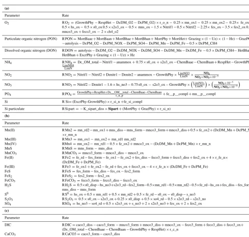
Figure 2.Simulated seasonal variability of the selected modeled chemical parameters (µM), in the water column (top panels) and in the
benthic boundary layer and sediments (bottom panels).
the reactions of particles in the sediments are assumed to have negligible impact on the volume fraction of total solids, and the deep particulate burial velocity w∞ in compacted
sediments (where ϕ=ϕ∞)is assumed to be a known
con-stant wb∞ (an input parameter). Since compaction ceases
at this (possibly infinite) depth, the solute burial velocity must here equal the particulate burial velocity (u∞=wb∞).
Steady state then implies the following burial velocities (Ap-pendix B):
w=(1−ϕ∞) (1−ϕ) wb∞−
1
(1−ϕ)D inter B
∂ϕ
∂z (6)
u=ϕ∞ ϕ wb∞+
1
ϕD inter B
∂ϕ
∂z, (7)
whereDBinter is the interphase bioturbation diffusivity, non-zero only at the SWI and only if bioturbation across the SWI is enabled. In the second approach, the reactions of the mod-eled particulate substances in the sediments modify the total solid volume fraction, and the modeled sinking fluxes from the water column modify the flux of solid volume at the SWI. The velocities in Eqs. (6) and (7) then define background ve-locities (wb,ub)due to non-modeled particulates. Assuming
steady-state compaction leads to the following corrections to the background burial velocities (see Appendix B):
w0= 1 (1−ϕ)
XNp
i
1
ρi
vf(i)Cˆsf(i)+ z
Z
Ri z0
dz0
u0=1 ϕ w
0
∞−(1−ϕ) w0, (9)
wherew0=w−wb,u0=u−ub,Npis the number of
par-ticulate variables,ρi is the density of theith particle type, vf(i)is the sinking velocity in the fluff layer,Cˆsf(i)is the
sus-pended particulate concentration in the fluff layer,Ri is the
particulate reaction term, and w0∞ is the correction to the
deep particulate burial velocity, in practice approximated by the deepest value ofw0. Since the suspended portionCˆsf(i)is
not explicitly modeled, it is approximated as the minimum of the particulate concentrations in the fluff layer and the layer immediately above. In our applications, we have found that Eqs. (8) and (9) can improve the realism of sediment organic matter distributions, mainly by increasing the burial rate following pelagic production and export events such as the spring bloom.
Finally, the process of bioirrigation, whereby benthic or-ganisms flush out their burrows with water from the sediment surface, is modeled as a non-local solute exchange (follow-ing Aller, 2001; Meile et al., 2001; Rutgers Van Der Loeff and Boudreau, 1997; Schlüter et al., 2000):
TbirrC(i)=αϕ
O2s
O2s+KO2s
ˆ Cf(i)−Ci
(for solutes), (10) whereα (z)is the bioirrigation rate in oxic conditions,Cˆf(i)is
the flushing concentration of solute in the fluff layer, and the Michaelis–Menten function again accounts for the suppres-sion of worm activity in anoxic conditions. The oxic bioir-rigation rateα (z)is parameterized as an exponential decay from the sediment surface as in Schlüter et al. (2000). The total mass transfer to/from the sediment column must be bal-anced by a flux into/out of the fluff layer (see Eq. 1):
Tbirr(i)=
1
hf O2s O2s+KO2s
zmax
Z
zSWI
αϕCi− ˆCf(i)
dz0
(for solutes), (11)
where hf is the thickness of the fluff layer and zmax is
the depth of the bottom of the modeled sediment column.
TbirrC(i), Tbirr(i)=0 for all particulate variables. 2.1.7 BROM-transport numerical integration
Equations (1)–(3) are integrated numerically over a single combined grid (water column plus sediments) and using the same model time step in both water column and sediments. All concentrations are stored internally and input/output in units [mmol m−3 total volume]. Time stepping follows an operator splitting approach (Butenschön et al., 2012): con-centrations are successively updated by contributions over one time step of diffusion, bioirrigation, reaction, and sed-imentation, in that order. If any state variable has any “not-a-number” values at the end of the time step then the program is terminated.
Diffusive updates are calculated either by a simple forward-time central-space (FTCS) algorithm or by a semi-implicit central-space algorithm adapted from a routine in the General Ocean Turbulence Model, GOTM (Umlauf et al., 2005). Bioirrigation and reaction updates are calculated from forward Euler time steps, using FABM to compute
Ri, and sedimentation updates are calculated using a simple
first-order upwind differencing scheme. After each update, Dirichlet boundary conditions (see below) are reimposed and all concentrations are low bounded by a minimum value (de-fault=10−11µM) to avoid negative values. Maximum dif-fusive and advective Courant numbers can optionally be out-put after every time step or when/if a not-a-number value is detected. Before starting the integration, the program calcu-lates Courant numbers due to eddy/molecular diffusion and returns a warning message if maximum values on any given day exceed 0.5 and the FTCS option is selected.
BROM-transport also provides an option to divide the dif-fusion and sedimentation updates into smaller time steps re-lated to the sources-minus-sinks time step by fixed factors, since the physical transport processes are often numerically limiting (Butenschön et al., 2012). The default time step is 0.0025 days or 216 s, which is much longer than the char-acteristic equilibration timescale of the CO2kinetics (Zeebe
and Wolf-Gladrow, 2001).
2.1.8 BROM-transport vertical grid
Figure 3.
2.1.9 BROM-transport initial conditions
Initial conditions for all concentrations in Eqs. (1)–(3) can be provided by either using the initialization values defined in the fabm.yaml file (see Sect. S2 in the Supplement) as uni-form initial conditions for each variable, or by providing the initial conditions for all variables at every depth in a text file with a specific format. Typically, these initial-condition text files are generated by running the model to a steady state annual cycle and saving the final values as the desired start date. Alternatively, they could be generated by interpolat-ing/smoothing data, in which case the user should note that the input concentrations must be in units [mmol m−3 total volume].
2.1.10 BROM-transport boundary conditions
BROM-transport presently allows the user to choose between four different types of boundary conditions for each variable and for upper and lower boundaries: (1) no gradient at the bottom boundary (no diffusive flux) or no flux at the surface boundary, except where parameterized by the FABM biogeo-chemical model (i.e., for O2and DIC in the case of
BROM-biogeochemistry); (2) a fixed constant value; (3) a fixed si-nusoidal variation in time defined by amplitude, mean value, and phase parameters; or (4) an arbitrary fixed variation in
time read from the input NetCDF file. All boundary condi-tion opcondi-tions and parameters are set in the brom.yaml file (see Sect. S1). Note that options 2–4 are Dirichlet boundary con-ditions which define implicit fluxes of matter into and out of the model domain, and that all boundary concentrations should be in units [mmol m−3total volume (water+solids)]. The default option 1 is generally the preferred choice, but the Dirichlet options can also be useful to allow a simple repre-sentation of, e.g., fluxes of nutrients into and out of the sur-face layer due to lateral riverine input. A possible alternative is to use the forcings’ parameters for horizontal mixing (see Eq. 1) to specify horizontal exchanges or restoring terms to observed climatology (see Sect. 2.2.7).
Under option 1, and using BROM-biogeochemistry, a sur-face O2 flux representing exchange with the atmosphere is
parameterized as
QO2=K660×
Sc
660
2
×(O2sat−O2) , (12)
where O2sat is the oxygen saturation as a function of
temperature and salinity, according to UNESCO (1986),
Sc is the Schmidt number for oxygen (Raymond et al., 2012), and k660 is the reference gas-exchange transfer
ve-locity, parameterized ask660=0.365u2+0.46u(Schneider
Figure 3.Vertical distributions of the modeled chemical parameters (µM), biological parameters (µM N), temperature (◦C), salinity (PSU), and vertical diffusivity (10−3m2s−1) during the winter period of well-mixed conditions, showing the water column (light blue), the benthic boundary layer (dark blue), and the sediments (light brown). Vertical distributions of the modeled chemical parameters (µM) and biological parameters (µM N) during the winter period of well-mixed conditions, showing the water column (light blue), the benthic boundary layer (dark blue), and the sediments (light brown).
sea surface (m s−1). Air–sea exchange of CO
2 in
BROM-biogeochemistry is parameterized using the partial pressures in water (pCOwater2 )and air (pCOair2 )following the formula-tion and coefficients in Butenschön et al. (2016):
QO2 =Fwind×
pCO2air−pCO2water
, (13)
where Fwind=(0.222u2+0.333u)(Sc/660)−0.5 is a wind
parameter (Nightingale et al., 2000),uis the wind speed, and
Scis the Schmidt number for CO2(Raymond et al., 2012). 2.1.11 BROM-transport irradiance model
BROM-transport includes two simple Beer–Lambert atten-uation models to calculate in situ 24 h average photosyn-thetically active radiation (PAR) as needed by BROM-biogeochemistry and many other biogeochemical models. The first is derived from the current ERSEM default model (Blackford et al., 2004; Butenschön et al., 2016) and models the total attenuation as
kt =k0+kPhyPhy+kPONPON+ksS, (14)
wherek0is the background attenuation of seawater,kPhyand kPONare the specific attenuations due to phytoplankton and
detritus, respectively, andks is the specific attenuation due
to “other” optically active substances with concentrationS
(currently a constant input parameter). The second model includes attenuation due to other optically active concentra-tions that are modeled by BROM-biogeochemistry:
kt=k0+kPhyPhy+kPONPON+kHetHet+kDONDON +kPBB+kPIVPIV+ksS, (15)
whereBis the total bacterial concentration (Baae+Baan+
Figure 4.
2.1.12 BROM-transport input forcings
BROM-transport requires forcing inputs at least for temper-ature, salinity, and vertical diffusivity at all depths in the pelagic water column and for each day of the simulation. These may be provided from an input subroutine that cre-ates simple, hypothetical profiles, or from text/NetCDF files containing data from interpolations of measurements or hy-drodynamic model output. Forcing time series of surface ir-radiance and ice thickness may also be read as NetCDF in-put. BROM-transport then uses these inputs in combination with parameters set in the runtime input file brom.yaml (see Sect. S1) to solve the transport-reaction equations on a “full” vertical grid including pelagic water column, BBL, and sed-iment subgrids.
In order to run, BROM-transport must extend the input pelagic (temperature, salinity, diffusivity) forcings over the full grid. Temperature and salinity in the BBL and sediments are set as uniform and equal to the values at the bottom of the input pelagic water column for each day. The vertical diffu-sivity needs a more careful treatment, as it is the main defin-ing characteristic of the pelagic vs. BBL vs. sediment envi-ronments. Within the water column, the total vertical diffu-sivityD=Dm+Defor solutes andD=Defor particulates,
whereDm is a constant molecular diffusivity at infinite
di-lution, and De is the eddy diffusivity read from the input
file for the pelagic water column. For the BBL, De can be
defined as “dynamic”, in which case it is linearly interpo-lated for each day between the deepest input forcing value above the SWI and zero at a depth hDBL above the SWI,
wherehDBLis the diffusive boundary layer (DBL) thickness
(default value 0.5 mm). This option is likely appropriate for shallow-water applications whereDe may be strongly time
dependent within the user-defined BBL (default thickness 0.5 m). Alternatively, a static, fixed profileDeBBL(z)may be
more appropriate for deep-water BBLs, where time depen-dence may be weak and deepest values from hydrodynamic models may be relatively far above the SWI. In this case, BROM-transport offers two options forDeBBL(z): (1) a
con-stant value, dropping to zero in the DBL, or (2) a linear vari-ation between a fixed value at the top of the BBL and zero at the top of the DBL. Option 1 defines a simplest-possible assumption, while option 2 corresponds to the assumption of a log layer for the current speed (e.g., Boudreau and Jor-gensen, 2001; Holtappels and Lorke, 2011). Eddy diffusivity is strictly zero in the DBL, on the SWI, and within the sed-iments. Diffusivity in the sediments is due to molecular dif-fusion and bioturbation and is parameterized as described in Sect. 2.2.1.