The potential of an observational data set for calibration of a computationally expensive computer model

(1)

www.geosci-model-dev.net/6/1715/2013/ doi:10.5194/gmd-6-1715-2013

Geoscientific

Model Development

The potential of an observational data set for calibration of

a computationally expensive computer model

D. J. McNeall1, P. G. Challenor2, J. R. Gattiker3, and E. J. Stone4

1_{Met Office Hadley Centre, Exeter, UK}

2_{College of Engineering, Mathematics and Physical Sciences, University of Exeter, Exeter, UK} 3_{Los Alamos National Laboratory, Los Alamos, New Mexico, NM 87545, USA}

4_{School of Geographical Sciences, University of Bristol, Bristol, UK}

Correspondence to: D. J. McNeall ([email protected])

Received: 15 February 2013 – Published in Geosci. Model Dev. Discuss.: 9 April 2013 Revised: 30 July 2013 – Accepted: 5 September 2013 – Published: 21 October 2013

Abstract. We measure the potential of an observational data

set to constrain a set of inputs to a complex and computation-ally expensive computer model. We use each member in turn of an ensemble of output from a computationally expensive model, corresponding to an observable part of a modelled system, as a proxy for an observational data set. We argue that, given some assumptions, our ability to constrain uncer-tain parameter inputs to a model using its own output as data, provides a maximum bound for our ability to constrain the model inputs using observations of the real system.

The ensemble provides a set of known parameter input and model output pairs, which we use to build a computation-ally efficient statistical proxy for the full computer model, termed an emulator. We use the emulator to find and rule out “implausible” values for the inputs of held-out ensemble members, given the computer model output. As we know the true values of the inputs for the ensemble, we can compare our constraint of the model inputs with the true value of the input for any ensemble member. Measures of the quality of constraint have the potential to inform strategy for data col-lection campaigns, before any real-world data is collected, as well as acting as an effective sensitivity analysis.

We use an ensemble of the ice sheet model Glimmer to demonstrate our measures of quality of constraint. The en-semble has 250 model runs with 5 uncertain input parame-ters, and an output variable representing the pattern of the thickness of ice over Greenland. We have an observation of historical ice sheet thickness that directly matches the output variable, and offers an opportunity to constrain the model. We show that different ways of summarising our

output variable (ice volume, ice surface area and maximum ice thickness) offer different potential constraints on individ-ual input parameters. We show that combining the observa-tional data gives increased power to constrain the model. We investigate the impact of uncertainty in observations or in model biases on our measures, showing that even a modest uncertainty can seriously degrade the potential of the obser-vational data to constrain the model.

1 Introduction

Computer models (referred to hereon as computer simula-tors) are used in a wide variety of computer experiments, for the understanding and prediction of real-world systems (see e.g. Santner et al., 2003 for examples). Such simula-tors contain uncertain parameters that may represent real but unknown physical constants, or be artefacts of the simplifi-cation (and therefore parameterization) of complex physical processes. It is important to choose an appropriate set of pa-rameters with which to run the simulator, in order that simu-lations match the behaviour of the true system as closely as possible.

(2)

extend this to cases where there are observations, but we could reduce their uncertainty. Finally, we might have a lim-ited budget, which we can choose to spend on reducing ob-servational uncertainty, or on improving the simulator – in effect, reducing the simulator discrepancy, or its associated uncertainty. To guide the observational campaign, we would like to know the potential of an observation, with a particular uncertainty, to constrain our simulator before we make the observation.

The comparison of simulators with observations from the appropriate real-world system, in order to choose a set of ap-propriate parameters, is known as calibration. This paper in-troduces a method for estimating the potential of a data set for calibrating a simulator, when that simulator is computa-tionally too expensive for brute force methods of calibration or tuning to be effective. We use an ensemble of the simu-lator output as a synthetic data set, treating output from an ensemble member as if it were an observation of the real sys-tem under study. We propose that our ability to calibrate the simulator when we know the true set of parameters (as in our ensemble), gives us a theoretical upper limit on our ability to calibrate the simulator in the real system.

In this synthetic test bed, we can examine the impact on the calibration of adding observational uncertainty, or simu-lator discrepancy uncertainty. We advise caution, as the true simulator discrepancy remains unknown, and might be dif-ferent from anything that we can reasonably simulate. How-ever, we believe that our metrics give a good guide to the maximum constraint possible, given a particular simulator, statistical framework, and data set.

Once a simulator is calibrated, it can be run to predict the behaviour of the system under untested circumstances. For example, climate simulators calibrated to historical data can be used to project and constrain the behaviour of the Earth system in the future under various greenhouse gas emission scenarios (Sexton et al., 2012; Sexton and Murphy, 2012; Rougier, 2007; Tebaldi and Knutti, 2007). Such simulators are often computationally expensive to run, such that there are usually only a small set of runs of the code with which to estimate a potentially large number of these uncertain but tuneable parameters within the simulator.

A probabilistic calibration allows for uncertainty in obser-vational data, and for the fact that the simulator does not per-fectly represent the true system. Such probabilistic calibra-tion allows a range for each of the input parameters, assign-ing a probability that each of the input parameters in a set might best match the simulator to the true system. In this case, a probabilistic prediction can be made by weighting the prediction of the simulator according to the probability of the corresponding set of input parameters being correct.

Metrics for the potential of data to constrain input parame-ters have been proposed when working with computationally cheap simulators and probabilistic calibration methods; for example to simulate atmospheric aerosols (Partridge et al., 2012), or terrestrial ecosystem models (Ziehn et al., 2012).

Here, we extend the methods for calculating these kinds of metrics to computationally expensive simulators.

Calibration of a computationally expensive simulator can be efficiently achieved using an emulator: a fast and compu-tationally cheap statistical proxy for the full simulator. Use of an emulator for calibration in a Bayesian setting was pi-oneered by Kennedy and O’Hagan (2001), with Wilkinson (2011) offering a review of recent developments. An alterna-tive approach, also using emulation techniques, is the history matching of Craig et al. (1996, 1997, 2001). History match-ing places more emphasis on rulmatch-ing out parameter sets where the simulator performs poorly, whereas probabilistic calibra-tion tends to down-weight poorly performing parameter sets. While these approaches differ in their interpretations of the meaning of the simulator, both share a notion of distance of simulator output from observations of the real system, as a measure of simulator quality.

Our metrics can also be viewed as a form of global sensi-tivity analysis (Saltelli et al., 2000). Sensisensi-tivity analysis (SA) in this context is concerned with quantifying the strength of the relationship between the inputs and outputs of a simula-tor. This relationship is often couched in terms of the induced change in simulator output, for a given change in simulator input. We are interested in inverting this measure, and finding the implied uncertainty of a simulator input, given an output. Trivially, if the output of a simulator is not sensitive to an in-put, then the data corresponding to the output will not have the power to constrain the input parameters. In addition, even where there may be a unique forward mapping from inputs to outputs of a simulator, this is not necessarily true of the in-verse mapping. A single output may have many correspond-ing inputs. An approach to probabilistic SA for expensive computer simulators is introduced by Oakley and O’Hagan (2004). Our approach draws on those techniques, particularly in the use of a Gaussian process emulator as a proxy for the computer simulator.

We first briefly introduce history matching as a method of solving inverse problems in the context of computer simula-tors in Sect. 2.1. We then introduce some empirical metrics for the ability of an observation to constrain the simulator input parameters in Sect. 2.2. In Sect. 2.3, we introduce em-ulators, and explain how they might be used in calculating the metrics introduced in the previous section. We apply our methods of constraint to an ensemble of a computationally expensive ice sheet simulator, and show that they work in Sect. 3. We introduce the results in Sect. 3.2, and discuss them and their implications for future research directions in Sect. 4. Finally, we offer some conclusions in Sect. 5.

(3)

2 Methods

2.1 Solving the inverse problem

We would like a metric for the strength of an observation of a system to calibrate (to constrain, or find good values for) a set of uncertain parameters in our computer simulator of that system. This equates to asking “how well can we solve the inverse problem, of estimating the parameters of a sim-ulator, given some data?”. There are at least two approaches to solving the inverse problem: probabilistic calibration, and history-matching techniques.

In a probabilistic calibration, a probability is assigned to a candidate set of inputs, depending on how well the corre-sponding output of the simulator matches observations, and the prior probability (before any data is seen) of the candidate point being “correct” in some manner.

Following Rougier (2007), we represent a particular set of d input parameters as vectorx=x1. . . xd, set within (∈) a “parameter” or “input” spaceX, judged to be plausible by the modeller, before the simulator is run. We assume that this plausible space corresponds to a “prior” probability dis-tribution, if we were to carry out a fully Bayesian analysis. Similarly, we represent the simulator output asy∈Y, repre-senting the state of some physical aspect of the system. We represent the simulator as a deterministic functiong(.), so that when run at a particular input parameter setx, it always returns the same value ofy. The simulator is complex enough that we cannot trivially predict the outputyat a givenx be-fore the simulator is run. We can represent outputy as an uncertain function of inputxthus:

y=g(x) . (1)

The relationship between the simulator outputy and an observationzof the real system is represented by the equa-tion

z=g(x∗)+δ(x∗)+e, (2) whereerepresents measurement errors in the observations, andδis the simulator discrepancy; the difference between the real system, and the simulator when run at its “best” input,

x∗_{. This best input is therefore defined as the point which} minimises the difference between the observations and the simulator output, given any known systematic errors (biases) in simulator discrepancy or in observations.

In calibrating the simulator, we compare a set of observa-tions of the true system,z, with the corresponding represen-tative output of the simulatory, and through the mapping in Eq. (1) we find a set of input parameters that is, by some mea-sure (but not necessarily all meamea-sures), good. In general, we assume that parameter sets which represent the real system well produce a smaller difference between simulator outputs

y and observations z, than do poor choices of inputs, and have a corresponding higher probability of representing the

best input. In addition, we assume that there are places within

X where it is possible to run the simulator, that nevertheless we judge as not well representing the true system being mod-elled. We would like to exclude these regions from our analy-sis as “implausible”, in effect setting their probability to zero. ConstrainingYto a smaller representative region by compar-ing it with observationsztherefore implies a constraint onX. This constraint might be achieved through a fully prob-abilistic calibration, simultaneously estimating probability distributions for x∗, and for simulator discrepancy δ, as in Kennedy and O’Hagan (2001). We use an alternative history-matching approach, based on the concept of implausibility, introduced by Craig et al. (1996). A full description of the benefits of history matching for expensive simulations can be found in Vernon et al. (2010). Briefly, the aim is to rule out as implausible, sets of parameters space where the simulator is a very poor fit to observations of the real system. Any set that is “not ruled out yet” is passed to further analysis. The im-plausibility measure must take into account (a) the fact that the observations are uncertain, (b) that we have uncertainty about ways in which the simulator might be wrong (the dis-crepancy), and (c) that we do not fully know the simulator behaviour, due to our limited ability to run the simulator.

We use an implausibility measureI that takes all of these uncertainties into account, writing

I2= |E

g(x)−z|2

Var

g(x)+δ(x)+e. (3)

An input is more implausible, the further the correspond-ing output lies from observations of the true system. How-ever, if the observations, the simulator output at that input, or the simulator discrepancy are more uncertain, that same input would be less implausible.

We regard any point where implausibility is below a threshold value of 3 as “not implausible”, and accept it as a candidate for the best input. This threshold comes from the 3σ rule of Pukelsheim (1994), which states that for unimodal distributions, ifx=x∗_{, then}_{I <}_{3, with a probability greater} than 0.95. This holds true even for highly skewed, or heavy-tailed distributions.

(4)

2.2 Metrics of constraint

We would like to assign a score or metric for the ability of a particular observationzof the real system to constrain our choice of a good set of input parameters within X. There are a number of ways that we might measure this, limited by some practical considerations. We propose two primary metrics: (1) the marginal range of plausible space in each input dimension, relative to the initial estimate and (2) the volume of “not implausible” input space, relative to the initial estimate.

2.2.1 Marginal range of “not implausible” input space

The marginal range R of an individual input is the largest range for each input parameter that we can find whereI <3. This is measured relative to the marginal ranges considered plausible before the simulator was run. While this measure can be useful as a simple sensitivity analysis, it should be treated with caution, and we regard it as inferior to the vol-ume of “not implausible” space metric, outlined in the next section. The range measures only the one-dimensional pro-jection of the “not implausible” input space. The true range of an individual might be very much smaller (and the metric correspondingly more useful), if we were to gain information about another input parameter, for example.

2.2.2 Volume of “not implausible input” space

We can define a volumeV of “not implausible” input pa-rameter space, or alternatively that input space “not ruled out yet” – as the region whereI <3. We can estimate the rela-tive volume of this space, with a Monte Carlo sample from the initially plausible spaceX. Using an indicator function

I(I <3), whereI=1 if true, and 0 if not, we taken sam-ples fromX, and estimate the volume as

V =1

n n

X

i=1

I(I <3) . (4)

We must be careful to take enough samples to ensure that this estimate is accurate, as well as taking into account the sometimes counter-intuitive nature of high dimensional space. For example, an observation that constrains the plausi-ble volume to half the range of each input in a 5-dimensional input space would have reduced the space to 0.55≈3 % of its original volume. However, such a reduction in volume can be achieved by constraining a single input to 3 % of its original range, with no constraint on any other input.

2.3 An emulator for computationally expensive

simulators

We are concerned with the case where the simulator is com-putationally expensive, and complex enough that we cannot trivially predict the output of the simulator before we run it.

We therefore cannot run the simulator enough times to com-prehensively explore the mapping ofX toY. We could, for example, run a collection of simulations in an optimisation routine to find x∗. This is unlikely to be a practical solu-tion, given the possibly complex nature ofz, the difficulty of searching high dimensional spaces which can have many lo-cal minima, and conflicting demands on expensive simulator output.

A more flexible solution is to run the simulator at a care-fully designed collection of points in X∈X, with associated output Y, called an ensemble, and use this to build a statis-tical model to predict the outputy, at untested points within

X. This statistical model, termed an emulator, is computa-tionally cheap and fast to run, and therefore can replace our simulator in any analysis of the ensemble. The emulator re-turns an estimated probability distribution for simulator out-put given an inout-put.

It is important to design the ensemble well, in order to build a good emulator. The simulator should provide good coverage of the input parameter space, in order that interac-tions between parameters might be well estimated. It should also span enough parameter space that the emulator is not called to extrapolate far beyond the design points, or param-eter values where the emulator has been validated. A good option is the Latin hypercube design of McKay et al. (1979), and its space-filling variants.

The emulator, denotedη(.), provides us with a complete mapping ofXtoY, with some uncertainty. If this uncertainty is tolerably small, we can use the emulated best estimate of simulated output in any analysis where we would normally use the simulator directly. We denote the best estimate fory

at any givenxasyˆ=η(x).

2.4 Using an ensemble to find an upper bound of

potential constraint

With an ensemble of a priori plausible simulator evaluations, we let the simulator outputy take the place of a theoretical observational data setzin our analysis. We estimate “not im-plausible” candidates forx∗for a given ensemble member, given its outputy. The candidates will span a region within the original input parameter space. We can calculate the met-rics of constraint for that region, introduced in Sect. 2.2, and also check that the true value ofx∗_{falls within the “not} im-plausible” region.

For computational efficiency, we let the emulatorη(.)take the place of our simulatorg(.). Simulator discrepancyδ(.) and observational errore(along with their respective uncer-tainties) are both zero in this setting, as we know the obser-vational data perfectly and we are using the same simulator across the ensemble. We can easily add in a simulator dis-crepancy or observational error of our choice, in order to test their impact on our ability to constrainx∗.

We use a leave-one-out cross-validation (LOOCV) style test on the ensemble, to find metrics of constraint at a sample

(5)

across input space. For each ensemble member in turni=

1. . . nwe treat the outputyifrom an ensemble member as an observation of the true system. We build an emulator, con-ditioned on the entire ensemble, except inputxi and output

yi. By finding the “not implausible” region, where our im-plausibility measureI <3 for each output in the ensemble

y1. . .yn, we can obtain a sample of possible constraints that an observation would give, if it were found to beyi.

We take a large Monte Carlo sample from the prior dis-tribution at a large number of points withinX, and use the emulator to predictyˆi at each candidate point. We then find the implausibilityI at each emulated input, given the uncer-tainty about the true value of the simulator at that point, pro-vided by the emulator. We calculate the metrics of plausible marginal input parameter rangeR, and plausible input space volumeV, using the emulated implausibility for each point.

Repeating this process across the ensemble, we obtain a sample ofnof each of the constraint metricsV1. . . Vn, and R1. . . Rn, where we havenensemble members. Each sample represents what the constraint might be if the true observation were to fall atyi, so we see that there is some uncertainty in the ability of the data to constrain the inputs, depending upon where in the ensemble the true data might fall.

It is important that the ensemble output spans a range wide enough to encompass any reasonable combination of obser-vation, simulator discrepancy and observational uncertainty. This is to avoid the situation where (for example) the obser-vation falls well outside the range of simulated output, and all of the input space is effectively ruled out immediately. In this situation, the analysis would be iterated, with new judge-ments about the uncertainty of simulator discrepancy.

3 An example using an ice sheet simulator

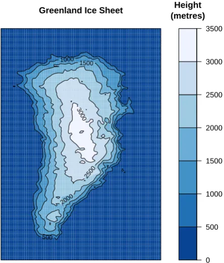
We investigate the utility of an emulator/observational data set combination, for the calibration of the ice sheet simulator Glimmer (version 1.04) (Rutt et al., 2009; Payne, 1999). We have access to an ensemble of 250 simulator runs, with 5 un-certain inputs, and an output variable, ice thickness, at each point in a 76×141 grid covering the Greenland Ice Sheet (GrIS). This ensemble was generated and examined in Stone et al. (2010); details of the inputs and outputs are summarised in Table 1. The simulator is sufficiently computationally ex-pensive to serve as a test bed for our methods, while being relatively straightforward to run in an ensemble of several hundred members.

The ensemble input points are sampled from independent uniform distributions of simulator inputs, using a Latin hy-percube sampling strategy. We normalize all inputs to a zero-one scale, based on the expert-elicited limits of the ensemble design.

The simulator output domain matches real-world observa-tions of ice sheet thickness (Bamber et al., 2001) interpo-lated to the simulator grid (Fig. 1), and shown here to aid

0 500 1000 1500 2000 2500 3000 3500 Height (metres)

500

1000 1500

2000 2500

3000

Greenland Ice Sheet

Fig. 1.

Observations of ice sheet thickness over the Glimmer domain, from Bamber et al. (2001).

24

Fig. 1. Observations of ice sheet thickness over the Glimmer

do-main, from Bamber et al. (2001).

interpretation of the data. We can summarise the output vari-able ice thickness, into a univariate output, in three ways. First, we can find ice volume (denoted ICEVOL), by sum-ming the ice thickness over the entire simulator domain. Sec-ond, we can take the surface area (ICESA) of the ice sheet. Third, we can examine the maximum thickness (MAXTHK) of the ice sheet. It is important to simulate all of these vari-ables correctly, in order to have confidence that our ice sheet simulator is capturing the relevant dynamics of the GrIS. In Fig. 2, we plot the marginal relationships between each pair of inputs and outputs. We see that, even though the summary outputs are from the same field variable, the output sum-maries are affected by input dimensions in different ways. Again, simulator outputs are normalized to a zero-one scale.

3.1 Building and checking the emulator

(6)

Table 1. Expert-elicited ranges for input parameters of Glimmer, and the corresponding ranges of the output parameters.

Units Abbrev. Min Max

Input Parameter

Positive degree day factor for snow mm d−1◦C−1 PDDFS 3 5 Positive degree day factor for ice mm d−1◦C−1 PDDFI 8 20 Near-surface lapse rate ◦C km−1 NSLR −8.2 −4

Flow enhancement factor – FEF 1 5

Geothermal heat flux mW m−2 GHF −61 −38

Output Parameter

Ice volume m3 ICEVOL 3.1×106 4.3×106

Ice surface area m2 ICESA 2.0×106 2.4×106 Maximum ice thickness m MAXTHK 3.0×103 3.7×106

0.0030 0.0040 0.0050

0.0030 0.0035 0.0040 0.0045 0.0050 PDDFS 0.008 0.010 0.012 0.014 0.016 0.018 0.020 ● ● ● ● ● ● ● ● ● ● ● ● ● ● ● ● ● ● ● ● ● ● ● ● ● ● ● ● ● ● ● ● ● ● ● ● ● ● ● ● ● ● ● ● ● ● ● ● ● ● ● ● ● ● ● ● ● ● ● ● ● ● ● ● ● ● ● ● ● ● ● ● ● ● ● ● ● ● ● ● ● ● ● ● ● ● ● ● ● ● ● ● ● ● ● ● ● ● ● ● ● ● ● ● ● ● ● ● ● ● ● ● ● ● ● ● ● ● ● ● ● ● ● ● ● ● ● ● ● ● ● ● ● ● ● ● ● ● ● ● ● ● ● ● ● ● ● ● ● ● ● ● ● ● ● ● ● ● ● ● ● ● ● ● ● ● ● ● ● ● ● ● ● ● ● ● ● ● ● ● ● ● ● ● ● ● ● ● ● ● ● ● ● ● ● ● ● ● ● ● ● ● ● ● ● ● ● ● ● ● ● ● ● ● ● ● ● ● ● ● ● ● ● ● ● ● ● ● ● ● ● ● ● ● ● ● ● ● ● ● ● ● ● ● ● ● ● ● ● ● PDDFI 4 5 6 7 8 ● ● ● ● ● ● ● ● ● ● ● ● ● ● ● ● ● ● ● ● ● ● ● ● ● ● ● ● ● ● ● ● ● ● ● ● ● ● ● ● ● ● ● ● ● ● ● ● ● ● ● ● ● ● ● ● ● ● ● ● ● ● ● ● ● ● ● ● ● ● ● ● ● ● ● ● ● ● ● ● ● ● ● ● ● ● ● ● ● ● ● ● ● ● ● ● ● ● ● ● ● ● ● ● ● ● ● ● ● ● ● ● ● ● ● ● ● ● ● ● ● ● ● ● ● ● ● ● ● ● ● ● ● ● ● ● ● ● ● ● ● ● ● ● ● ● ● ● ● ● ● ● ● ● ● ● ● ● ● ● ● ● ● ● ● ● ● ● ● ● ● ● ● ● ● ● ● ● ● ● ● ● ● ● ● ● ● ● ● ● ● ● ● ● ● ● ● ● ● ● ● ● ● ● ● ● ● ● ● ● ● ● ● ● ● ● ● ● ● ● ● ● ● ● ● ● ● ● ● ● ● ● ● ● ● ● ● ● ● ● ● ● ● ● ● ● ● ● ● ● ● ● ● ● ● ● ● ● ● ● ● ● ● ● ● ● ● ● ● ● ● ● ● ● ● ● ● ● ● ● ● ● ● ● ● ● ● ● ● ● ● ● ● ● ● ● ● ● ● ● ● ● ● ● ● ● ● ● ● ● ● ● ● ● ● ● ● ● ● ● ● ● ● ● ● ● ● ● ● ● ● ● ● ● ● ● ● ● ● ● ● ● ● ● ● ● ● ● ● ● ● ● ● ● ● ● ● ● ● ● ● ● ● ● ● ● ● ● ● ● ● ● ● ● ● ● ● ● ● ● ● ● ● ● ● ● ● ● ● ● ● ● ● ● ● ● ● ● ● ● ● ● ● ● ● ● ● ● ● ● ● ● ● ● ● ● ● ● ● ● ● ● ● ● ● ● ● ● ● ● ● ● ● ● ● ● ● ● ● ● ● ● ● ● ● ● ● ● ● ● ● ● ● ● ● ● ● ● ● ● ● ● ● ● ● ● ● ● ● ● ● ● ● ● ● ● ● ● ● ● ● ● ● ● ● ● ● ● ● ● ● ● ● ● ● ● ● ● ● ● NSLR 1 2 3 4 5 ● ● ● ● ● ● ● ● ● ● ● ● ● ● ● ● ● ● ● ● ● ● ● ● ● ● ● ● ● ● ● ● ● ● ● ● ● ● ● ● ● ● ● ● ● ● ● ● ● ● ● ● ● ● ● ● ● ● ● ● ● ● ● ● ● ● ● ● ● ● ● ● ● ● ● ● ● ● ● ● ● ● ● ● ● ● ● ● ● ● ● ● ● ● ● ● ● ● ● ● ● ● ● ● ● ● ● ● ● ● ● ● ● ● ● ● ● ● ● ● ● ● ● ● ● ● ● ● ● ● ● ● ● ● ● ● ● ● ● ● ● ● ● ● ● ● ● ● ● ● ● ● ● ● ● ● ● ● ● ● ● ● ● ● ● ● ● ● ● ● ● ● ● ● ● ● ● ● ● ● ● ● ● ● ● ● ● ● ● ● ● ● ● ● ● ● ● ● ● ● ● ● ● ● ● ● ● ● ● ● ● ● ● ● ● ● ● ● ● ● ● ● ● ● ● ● ● ● ● ● ● ● ● ● ● ● ● ● ● ● ● ● ● ● ● ● ● ● ● ● ● ● ● ● ● ● ● ● ● ● ● ● ● ● ● ● ● ● ● ● ● ● ● ● ● ● ● ● ● ● ● ● ● ● ● ● ● ● ● ● ● ● ● ● ● ● ● ● ● ● ● ● ● ● ● ● ● ● ● ● ● ● ● ● ● ● ● ● ● ● ● ● ● ● ● ● ● ● ● ● ● ● ● ● ● ● ● ● ● ● ● ● ● ● ● ● ● ● ● ● ● ● ● ● ● ● ● ● ● ● ● ●● ● ● ● ● ● ● ● ● ● ● ● ● ● ● ● ● ● ● ● ● ● ● ● ● ● ● ● ● ● ● ● ● ● ● ● ● ● ● ● ● ● ● ● ● ● ● ● ● ● ● ● ● ● ● ● ● ● ● ● ● ● ● ● ● ● ● ● ● ● ● ● ● ● ● ● ● ● ● ● ● ● ● ● ● ● ● ● ● ● ● ● ● ● ● ● ● ● ● ● ● ● ● ● ● ● ● ● ●● ● ● ● ● ● ● ● ● ● ● ● ● ● ● ● ● ● ● ● ● ● ● ● ● ● ● ● ● ● ● ● ● ● ● ● ● ● ● ● ● ● ● ● ● ● ● ● ● ● ● ● ● ● ● ● ● ● ● ● ● ● ● ● ● ● ● ● ● ● ● ● ● ● ● ● ● ● ● ● ● ● ● ● ● ● ● ● ● ● ● ● ● ● ● ● ● ● ● ● ● ● ● ● ● ● ● ● ● ● ● ● ● ● ● ● ● ● ● ● ● ● ● ● ● ● ● ● ● ● ● ● ● ● ● ● ● ● ● ● ● ● ● ● ● ● ● ● ● ● ● ● ● ● ● ● ● ● ● ● ● ● ● ● ● ● ● ● ● ● ● ● ● ● ● ● ● ● ● ● ● ● ● ● ● ● ● ● ● ● ● ● ● ● ● ● ● ● ● ● ● ● ● ● ● ● ● ● ● ● ● ● ● ● ● ● ● ● ● ● ● ● ● ● ● ● ● ● ● ● ● ● ● ● ● ● ● ● ● ● ● ● ● ● ● ● ● ● ● ● ● ● ● ● ● ● ● ● ● ● ● ● ● ● ● ● ● ● ● ● ● ● ● ● ● ● ● ● ● FEF −0.060 −0.055 −0.050 −0.045 −0.040 ● ● ● ● ● ● ● ● ● ● ● ● ● ● ● ● ● ● ● ● ● ● ● ● ● ● ● ● ● ● ● ● ● ● ● ● ● ● ● ● ● ● ● ● ● ● ● ● ● ● ● ● ● ● ● ● ● ● ● ● ● ● ● ● ● ● ● ● ● ● ● ● ● ● ● ● ● ● ● ● ● ● ● ● ● ● ● ● ● ● ● ● ● ● ● ● ● ● ● ● ● ● ● ● ● ● ● ● ● ● ● ● ● ● ● ● ● ● ● ● ● ● ● ● ● ● ● ● ● ● ● ● ● ● ● ● ● ● ● ● ● ● ● ● ● ● ● ● ● ● ● ● ● ● ● ● ● ● ● ● ● ● ● ● ● ● ● ● ● ● ● ● ● ● ● ● ● ●● ● ● ● ● ● ● ● ● ● ● ● ● ● ● ●● ● ● ● ● ● ● ● ● ● ● ● ● ● ● ● ● ● ● ● ● ● ● ● ● ● ● ● ● ● ● ● ● ● ● ● ● ● ● ● ● ● ● ● ● ● ● ● ● ● ● ● ● ● ● ● ●● ● ● ● ● ● ● ● ● ● ● ● ● ● ● ● ● ● ● ● ● ● ● ● ● ● ● ● ● ● ● ● ● ● ● ● ● ● ● ● ● ● ● ● ● ● ● ● ● ● ● ● ● ● ● ● ● ● ● ● ● ● ● ● ● ● ● ● ● ● ● ● ● ● ● ● ● ● ● ● ● ● ● ● ● ● ● ● ● ● ● ● ● ● ● ● ● ● ● ● ● ● ● ● ● ● ● ● ● ● ● ● ● ● ● ● ● ● ● ● ● ● ● ● ● ● ● ● ● ● ● ● ● ● ● ● ● ● ● ● ● ● ● ● ● ● ● ● ● ● ● ● ● ● ● ● ● ● ● ● ● ● ● ● ● ● ● ● ● ● ● ● ● ● ● ● ● ● ● ● ● ● ● ● ● ● ● ● ● ● ● ● ● ● ● ● ● ● ● ● ● ● ● ● ● ● ● ● ● ● ● ● ● ● ● ● ● ● ● ● ● ● ● ● ● ● ● ● ● ● ● ● ● ● ● ● ● ● ● ● ● ● ● ● ● ● ● ● ● ●● ● ● ● ● ● ● ● ● ● ● ● ● ● ● ● ● ● ● ● ● ● ● ● ● ● ● ● ● ● ● ● ● ● ● ● ● ● ● ● ● ● ● ● ● ● ● ● ● ● ● ● ● ● ● ● ● ● ● ● ● ● ● ● ● ● ● ● ● ● ● ● ● ● ● ● ● ● ● ● ● ● ● ● ● ● ● ● ● ● ● ● ● ● ● ● ● ● ● ● ● ● ● ● ● ● ● ● ● ● ● ● ● ● ● ● ● ● ● ● ● ● ● ● ● ● ● ● ● ● ●● ● ● ● ● ● ● ● ● ● ● ● ● ● ● ● ● ● ● ● ● ● ● ● ● ● ● ● ● ● ● ● ● ● ● ● ● ● ● ● ● ● ● ● ● ●● ● ● ● ● ● ● ● ● ● ● ● ● ● ● ● ● ● ● ● ● ● ● ● ● ● ● ● ● ● ● ● ● ● ● ● ● ● ● ● ● ● ● ● ● ● ● ● ● ● ● ● ● ● ● ● ● ● ● ● ● ● ● ● ● ● ● ● ● ● ● ● ● ● ● ● ● ● ● ● ● ● ● ● ● ● ● ● ● ● ● ● ● ● ● ● ● ● ● ● ● ● ● ● ● ● ● ● ● ● ● ● ● ● ● ● ● ● ● ● ● ● ● ● ● ● ● ● ● ● ● ● ● ● ● ● ● ● ● ● ● ● ● ● ● ● ● ● ● ● ● ● ● ● ● ● ● ● ● ● ● ● ● ● ● ● ● ● ● ● ● ● ● ● ● ● ● ● ● ● ● ● ● ● ● ● ● ● ● ● ● ● ● ● ● ● ● ● ● ● ● ● ● ● ● ● ● ● ● ● ● ● ● ● ● ● ● ● ● ● ● ● ● ● ● ● ● ● ● ● ● ● ● ● ● ● ● ● ● ● ● ● ● ● ● ● ● ● ● ● ● ● ● ● ● ● ● ● ● ● ● ● ● ● ● ● ● ● ● ● ● ● ● ● ● ● ● ● ● ● ● ● ● ● ● ● ● ● ●● ● ● ● ● ● ● ● ● ● ● ● ● ● ● ● ● ● ● ●● ● ● ● ● ● ● ● ● ● ● ● ● GHF 3200000 3400000 3600000 3800000 4000000 4200000 ● ● ● ● ● ● ● ● ● ● ● ● ● ● ● ● ● ● ● ● ● ● ● ● ● ● ● ● ● ● ● ● ● ● ● ● ● ● ● ● ● ● ● ● ● ● ● ● ●● ● ● ● ● ● ● ● ● ● ● ● ● ● ● ● ● ● ● ● ● ● ● ● ● ● ● ● ● ● ● ● ● ● ● ● ● ● ● ● ● ● ● ● ● ●● ● ● ● ● ● ● ● ● ● ● ● ● ● ● ● ● ● ● ● ● ● ● ● ● ● ● ● ● ● ● ● ● ● ● ● ● ● ● ● ● ● ● ● ● ● ● ● ● ● ● ● ● ● ● ● ● ● ● ● ● ● ● ● ● ● ● ● ● ● ● ● ● ● ● ● ● ● ● ● ● ● ● ● ● ● ● ● ● ● ● ● ● ● ● ● ● ● ● ● ● ● ● ● ● ● ● ● ● ● ● ● ● ● ● ● ● ● ● ● ● ● ● ● ● ● ● ● ● ● ● ● ● ● ● ● ● ● ● ● ● ● ● ● ● ● ● ● ● ● ● ● ● ● ● ● ● ● ● ● ● ● ● ● ● ● ● ● ● ● ● ● ● ● ● ● ● ● ● ● ● ● ● ● ● ● ● ● ● ● ● ● ● ● ● ● ● ● ●● ● ● ● ● ● ● ● ● ● ● ● ● ● ● ● ● ● ● ● ● ● ● ● ● ● ● ● ● ● ● ● ●●● ● ● ● ● ● ● ● ● ● ● ● ● ● ● ● ● ●● ● ● ● ● ● ● ● ● ● ● ● ● ● ● ● ● ● ● ● ● ● ● ● ● ● ● ● ● ● ● ● ● ● ● ● ● ● ● ● ● ● ● ● ● ● ● ● ● ● ● ● ● ● ● ● ● ● ● ● ● ● ● ● ● ● ● ● ● ● ● ● ● ● ● ● ● ● ● ● ● ● ● ● ● ● ● ● ● ● ● ● ● ● ● ● ● ● ● ● ● ● ● ● ● ● ● ● ● ● ● ● ● ● ● ● ● ● ● ● ● ● ● ● ● ● ● ● ● ● ● ● ● ● ● ● ● ● ● ● ● ● ● ● ● ● ● ● ● ● ● ● ● ● ● ● ● ● ● ● ● ● ● ● ● ● ● ● ● ● ● ● ● ● ● ● ● ● ● ● ● ● ● ● ● ● ● ● ● ● ● ● ● ● ● ● ● ●● ● ● ● ● ● ● ● ● ● ● ● ● ● ● ● ● ● ● ● ● ● ● ● ● ● ● ● ● ● ● ● ● ● ● ● ● ● ● ● ● ● ● ● ● ● ● ● ● ● ● ● ● ● ● ● ● ● ● ● ● ● ● ● ● ● ● ● ● ● ● ● ● ● ● ● ● ● ● ● ● ● ● ● ● ● ● ● ● ● ● ● ● ● ● ● ● ● ● ● ● ● ● ● ● ● ● ● ● ● ● ● ● ● ● ● ● ● ● ● ● ● ● ● ● ● ● ● ● ● ● ● ● ● ● ● ● ● ● ● ● ● ● ● ● ● ● ● ● ● ● ● ● ● ● ● ● ● ● ● ● ● ● ● ● ● ● ● ● ● ● ● ● ● ● ● ● ● ● ● ● ● ● ● ● ● ● ● ● ● ● ● ● ● ● ● ● ● ● ● ● ● ● ● ● ● ● ● ● ● ● ● ● ● ● ● ● ● ● ● ● ● ●● ● ● ● ● ● ● ● ● ● ● ● ● ● ● ● ● ● ● ● ● ● ● ● ● ● ●● ● ● ● ● ● ● ● ● ● ● ● ● ● ● ● ● ● ● ● ● ● ● ● ● ● ● ● ● ● ● ● ● ●● ● ● ● ● ● ● ● ● ● ● ● ● ● ● ● ●●● ● ● ● ● ● ● ● ● ● ● ● ● ● ● ● ● ● ● ● ● ● ● ● ● ● ● ● ● ● ● ● ● ● ● ● ● ● ● ● ● ● ● ● ● ● ● ● ● ● ● ● ● ● ● ● ● ● ● ● ● ● ● ● ● ● ● ● ● ● ● ● ● ● ● ● ● ● ● ● ● ● ● ● ● ● ● ● ● ● ● ● ● ● ● ● ● ● ● ● ● ● ● ● ● ● ● ● ● ● ● ● ● ● ● ● ● ● ● ● ● ● ● ● ● ● ● ● ● ● ● ● ● ● ● ● ● ● ● ● ● ● ● ● ● ● ● ● ● ● ● ● ● ● ● ● ● ● ● ● ● ● ● ● ● ● ● ● ● ● ● ● ● ● ● ● ● ● ● ● ● ● ● ● ● ● ● ● ● ● ● ● ● ● ● ● ● ● ● ● ● ● ●● ● ● ● ● ● ● ● ● ● ● ● ● ● ● ● ● ● ● ● ● ● ● ● ● ● ● ● ● ● ● ● ● ● ● ● ● ● ● ● ●● ● ● ● ● ● ● ● ● ● ● ● ● ● ● ● ● ● ● ● ● ● ● ●● ● ● ● ● ● ● ● ● ● ● ● ● ● ● ● ● ● ● ● ● ● ● ● ● ● ● ● ● ● ● ● ● ● ● ● ● ● ● ● ● ● ● ● ● ● ● ● ● ● ● ● ● ● ● ● ● ● ● ● ● ● ● ● ● ● ● ● ● ● ● ● ● ● ● ● ● ● ● ● ● ● ● ● ● ● ● ● ● ● ● ● ● ● ● ● ●● ● ● ● ● ● ● ● ● ● ● ● ● ● ● ● ● ● ● ● ● ● ● ● ● ● ● ● ● ● ● ● ● ● ● ● ● ● ● ICEVOL 2000000 2100000 2200000 2300000 ● ● ● ● ● ● ● ● ● ● ● ● ● ● ● ● ● ● ● ● ● ● ● ● ● ● ● ● ● ● ● ● ● ● ● ● ● ● ● ● ● ● ● ● ● ● ● ● ● ●● ● ● ● ● ● ● ● ● ● ● ● ● ● ● ● ● ● ● ● ● ● ● ● ● ● ● ● ● ● ● ● ● ● ● ● ● ● ● ● ● ● ● ● ● ● ● ● ● ● ● ● ● ● ● ● ● ● ● ● ● ● ● ● ● ● ● ● ● ● ● ● ● ● ● ● ● ● ● ● ● ● ● ● ● ● ● ● ● ● ● ● ● ● ● ● ● ● ● ● ● ● ● ● ● ● ● ● ● ● ● ● ● ● ● ● ● ● ● ● ● ● ● ● ● ● ● ● ● ● ● ● ● ● ● ● ● ● ● ● ● ● ● ● ● ● ●● ● ● ● ● ● ● ● ● ● ● ● ● ● ● ● ● ● ● ● ● ● ● ● ● ● ● ● ● ● ● ● ● ● ● ● ● ● ● ● ● ● ● ● ● ● ● ● ● ● ● ● ● ● ● ● ● ● ● ● ● ● ● ● ● ● ● ● ● ● ● ● ● ● ● ● ● ● ● ● ● ● ● ● ● ● ● ● ● ● ● ● ● ● ● ● ● ● ● ● ● ● ● ● ● ● ● ● ● ● ● ● ● ● ● ● ● ● ● ● ● ● ● ● ● ● ● ● ● ● ● ● ● ● ● ● ● ● ● ● ● ● ● ● ● ● ● ● ● ● ● ● ● ● ● ● ● ● ● ● ● ● ● ● ● ● ● ● ● ● ● ● ● ● ● ● ● ● ● ● ● ● ● ● ● ● ● ● ● ● ● ● ● ● ● ● ● ● ● ● ● ● ● ● ● ● ● ● ● ● ● ● ● ● ● ● ● ● ● ● ● ● ● ● ● ● ● ● ● ● ● ● ● ● ● ● ● ● ● ● ● ● ● ● ● ● ● ● ● ● ● ● ● ● ● ● ● ● ● ● ● ● ● ● ● ● ● ● ● ● ● ● ● ● ● ● ● ● ● ● ● ● ● ● ● ● ● ● ● ● ● ● ● ● ● ● ● ● ● ● ● ● ● ● ● ● ● ● ● ● ● ● ● ● ● ● ● ● ● ● ● ● ● ● ● ● ● ● ● ● ● ● ● ● ● ● ● ● ● ● ● ● ● ● ● ● ●● ● ● ● ● ● ● ● ● ● ● ● ● ● ● ● ● ● ● ● ● ● ● ● ● ● ● ● ●● ● ● ● ● ● ● ● ● ● ● ● ● ● ● ● ● ● ● ● ● ● ● ● ● ● ● ● ● ● ● ● ● ● ● ● ● ● ● ● ● ● ● ● ● ● ● ● ● ● ● ● ● ● ● ● ● ● ● ● ● ● ● ● ● ● ● ● ● ● ● ● ● ● ● ● ● ● ● ● ● ● ● ● ● ● ● ● ● ● ● ● ● ● ● ● ● ● ● ● ● ● ● ● ● ● ● ● ● ● ● ● ● ● ● ● ● ● ● ● ● ● ● ● ● ● ● ● ● ● ● ● ● ● ● ● ● ● ● ● ● ● ● ● ● ● ● ● ● ● ● ● ● ● ● ● ● ● ● ● ● ● ● ● ● ● ● ● ● ● ● ● ● ● ● ● ● ● ● ● ● ● ● ● ● ● ● ● ● ● ● ● ● ● ● ● ● ● ● ● ● ● ● ● ● ● ● ● ● ● ● ● ● ● ● ● ● ● ● ● ● ● ● ● ● ● ● ● ● ● ● ● ● ● ● ● ● ● ● ● ● ● ● ● ● ● ● ● ● ●● ● ● ● ● ● ● ● ● ● ● ● ● ● ● ● ● ● ● ● ● ● ● ● ● ● ● ● ● ● ● ● ● ● ● ● ● ● ● ● ● ● ● ● ● ● ● ● ● ● ● ● ● ● ● ● ● ● ● ● ● ● ● ● ● ● ● ● ● ● ● ● ● ● ● ● ● ● ● ● ● ● ● ● ● ● ● ● ● ● ● ● ● ● ● ● ● ● ● ● ● ● ● ● ● ● ● ● ● ● ● ● ● ● ● ● ● ● ● ● ● ● ● ● ● ● ● ● ● ● ● ● ● ● ● ● ● ● ● ● ● ● ● ● ● ● ● ● ● ● ● ● ● ● ● ● ● ● ● ● ● ● ● ● ● ● ● ● ● ● ● ● ● ● ● ● ● ● ● ● ● ● ● ● ● ● ● ● ● ● ● ● ● ● ● ● ● ● ● ● ● ● ● ● ● ● ● ● ● ● ● ● ● ● ● ● ● ● ● ● ● ● ● ● ● ● ● ● ● ● ● ● ● ● ● ● ● ● ● ●● ● ● ● ● ● ● ● ● ● ● ● ● ● ● ● ● ● ● ● ● ● ● ● ● ● ● ● ● ● ● ● ● ● ● ● ● ● ● ● ● ● ● ● ● ● ● ● ● ● ● ● ● ● ● ● ● ● ● ● ● ● ● ● ● ● ● ● ● ● ● ● ● ● ● ● ● ● ● ● ● ● ● ● ● ● ●● ● ● ● ● ● ● ● ● ● ● ● ● ● ● ● ● ● ● ● ● ● ● ● ● ● ● ● ● ● ● ● ● ● ● ● ● ● ● ● ● ● ● ● ● ● ● ●● ● ● ● ● ● ● ● ● ● ● ● ● ● ● ● ● ● ● ● ● ● ● ● ● ● ● ● ● ● ● ● ● ● ● ● ● ● ● ● ● ● ● ● ● ● ● ● ● ● ● ● ● ● ● ● ● ● ● ● ● ● ● ● ● ● ● ● ● ● ● ● ● ● ● ● ● ● ● ● ● ● ● ● ● ● ● ● ● ● ● ● ● ● ● ●● ● ● ● ● ● ● ● ● ● ● ● ● ● ● ● ● ● ● ● ● ● ● ● ● ● ● ● ● ● ● ● ● ● ● ● ● ● ● ● ● ● ● ● ● ● ● ● ● ● ● ● ● ● ● ● ● ● ● ● ● ● ● ● ● ● ● ● ● ● ● ● ● ● ● ● ● ● ● ● ● ● ● ● ● ● ● ● ● ● ● ● ● ● ● ● ● ● ● ● ● ● ● ● ● ● ● ● ● ● ● ● ● ● ● ● ● ● ● ● ● ● ● ● ● ● ● ● ● ● ● ● ● ● ● ● ● ● ● ● ● ● ● ● ● ● ● ● ● ● ● ● ● ●● ● ● ● ● ● ● ● ● ● ● ● ● ● ● ● ● ● ● ● ● ● ● ● ● ● ● ●● ● ● ● ● ● ● ● ● ● ● ● ● ● ● ● ● ● ● ● ● ● ● ● ICESA

0.0030 0.0040 0.0050 3000 3100 3200 3300 3400 3500 3600 3700 ● ● ● ● ● ● ● ● ● ● ● ● ● ● ● ● ● ● ● ● ● ● ● ● ● ● ● ● ● ● ● ● ● ● ● ● ● ● ● ● ● ● ● ● ● ● ● ● ● ● ● ● ● ● ● ● ● ● ● ● ● ● ● ● ● ● ● ● ● ● ● ● ● ● ● ● ● ● ● ● ● ● ● ● ● ● ● ● ● ● ● ● ● ● ● ● ● ● ● ● ● ● ● ● ● ● ● ● ● ● ● ● ● ● ● ● ● ● ● ● ● ● ● ● ● ● ● ● ● ● ● ● ● ● ● ● ● ● ● ● ● ● ● ● ● ● ● ● ● ● ● ● ● ● ● ● ● ● ● ● ● ● ● ● ● ● ● ● ● ● ● ● ● ● ● ● ● ● ● ● ● ● ● ● ● ● ● ● ● ● ● ● ● ● ● ● ● ● ● ● ● ● ● ● ● ● ● ● ● ● ● ● ● ● ● ● ● ● ● ● ● ● ● ● ● ● ● ● ● ● ● ● ● ● ● ● ● ● ● ● ● ● ● ● ● ● ● ● ● ●

0.008 0.014 0.020

● ● ● ● ● ● ● ● ● ● ● ● ● ● ● ● ● ● ● ● ● ● ● ● ● ● ● ● ● ● ● ● ● ● ● ● ● ● ● ● ● ● ● ● ● ● ● ● ● ● ● ● ● ● ● ● ● ● ● ●● ● ● ● ● ● ● ● ● ● ● ● ● ● ● ● ● ● ● ● ● ● ● ● ● ● ● ● ● ● ● ● ● ● ● ● ● ● ● ● ● ● ● ● ● ● ● ● ● ● ● ●● ● ● ● ● ● ● ● ● ● ● ● ● ● ● ● ● ● ● ● ● ● ● ● ● ● ● ● ● ● ● ● ● ● ● ● ● ● ● ● ● ● ● ● ● ● ● ● ● ● ● ● ● ● ● ● ● ● ● ● ● ● ● ● ● ● ● ● ● ● ● ● ● ● ● ● ● ● ● ● ● ● ● ● ● ● ● ● ● ● ● ● ● ● ● ● ● ● ● ● ● ● ● ● ● ●● ● ● ● ● ● ● ● ● ● ● ● ● ● ● ● ● ● ● ● ● ● ● ● ● ● ● ● ● ● ● ●

4 5 6 7 8

● ● ● ● ● ● ● ● ● ● ● ● ● ● ● ● ● ● ● ● ● ● ● ● ● ● ● ● ● ● ● ● ● ● ● ● ● ● ● ● ● ● ● ●● ● ● ● ● ● ● ● ● ● ● ● ● ● ● ● ● ● ● ● ● ● ● ● ● ● ● ● ● ● ● ● ● ● ● ● ● ● ● ● ● ● ● ● ● ● ● ● ● ● ● ● ● ● ● ● ● ● ● ● ● ● ● ● ● ● ● ● ● ● ● ● ● ● ● ● ● ● ● ● ● ● ● ● ● ● ● ● ● ● ● ● ● ● ● ● ●● ● ● ● ● ● ● ● ● ● ● ● ● ● ● ● ● ● ● ● ● ● ● ● ● ● ● ● ● ● ● ● ● ● ● ● ● ● ● ● ● ● ● ● ● ● ● ● ● ● ● ●● ● ● ● ● ● ● ● ● ● ● ● ● ● ● ● ● ● ● ● ● ● ● ● ● ●● ● ● ● ● ● ● ● ● ● ● ● ● ● ● ● ● ● ● ● ● ● ● ● ● ● ● ● ● ● ●

1 2 3 4 5

● ● ● ● ● ● ● ● ● ● ● ● ● ● ● ● ● ● ● ● ● ● ● ● ● ● ● ● ● ● ● ● ● ● ● ● ● ● ● ● ● ● ● ● ● ● ● ● ● ● ● ● ● ● ● ● ● ● ● ● ● ● ● ● ● ● ● ● ● ● ● ● ● ● ● ● ● ● ● ● ●● ● ● ● ● ● ●● ● ● ● ● ● ● ● ● ● ● ● ● ● ● ● ● ● ● ● ● ● ● ● ● ● ● ● ● ● ● ● ● ● ● ● ● ● ● ● ● ● ● ● ● ● ● ● ● ● ● ●● ● ● ● ● ● ● ● ● ● ● ● ● ● ● ● ● ● ● ● ● ● ● ● ● ● ● ● ● ● ● ● ● ● ● ● ● ● ● ● ● ● ● ● ● ● ● ● ● ● ● ● ● ● ● ● ● ● ● ● ● ● ● ● ● ● ● ● ● ● ● ● ● ● ● ● ●● ●● ● ● ● ● ● ● ● ● ● ● ● ● ● ● ● ● ● ● ● ● ● ● ● ● ● ● ● ● ● ●

−0.060 −0.050 −0.040

● ● ● ● ● ● ● ● ● ● ● ● ● ● ● ● ● ● ● ● ● ● ● ● ● ● ● ● ● ● ● ● ● ● ● ● ● ● ● ● ● ● ● ● ● ● ● ● ● ● ● ● ● ● ● ● ● ● ● ● ● ● ● ● ● ● ● ● ● ● ● ● ● ● ● ● ● ● ● ● ● ● ● ● ● ● ● ● ● ● ● ● ● ● ● ● ● ● ● ● ● ● ● ● ● ● ● ● ● ● ● ●● ● ● ● ● ● ● ● ● ● ● ● ● ● ● ● ● ● ● ● ● ● ● ● ● ● ● ● ●● ● ● ● ● ● ● ● ● ● ● ● ● ● ● ● ● ● ● ● ● ● ● ● ● ● ● ● ● ● ● ● ● ● ● ● ● ● ● ● ● ● ● ● ● ● ● ● ● ● ● ● ● ● ● ● ● ● ● ● ● ● ● ● ● ● ● ● ● ● ● ● ● ● ● ● ● ● ● ● ● ● ● ● ● ● ● ● ● ● ● ● ● ● ● ● ● ● ● ● ● ● ● ● ● ● ● ● ● 3200000 4000000 ● ● ● ● ● ● ● ● ● ● ● ● ● ● ● ● ●● ● ● ● ● ● ● ● ● ● ● ● ● ● ● ● ● ● ● ● ● ● ● ● ● ● ●● ● ● ● ● ● ● ● ● ● ● ● ● ● ● ● ● ● ● ● ● ● ● ● ● ● ● ● ● ● ● ● ● ● ● ● ● ● ● ● ● ● ● ●● ● ● ● ● ● ● ● ● ● ● ● ● ● ● ● ● ● ● ● ● ● ● ● ● ● ● ● ● ● ● ● ● ● ● ● ● ● ● ● ● ● ● ● ● ● ● ● ● ● ● ● ● ● ● ● ● ● ● ● ● ● ● ● ● ● ● ● ● ● ● ● ● ● ● ● ● ● ● ● ● ● ● ● ● ● ● ● ● ● ● ● ● ● ● ● ● ● ● ● ● ● ● ● ●● ● ● ● ● ● ● ● ● ● ● ● ● ● ● ● ● ● ● ● ● ● ● ●●●● ● ● ● ● ● ● ● ● ● ● ● ● ● ● ● ● ● ● ● ● ● ● ● ● ● ● ● ● ● ● 2000000 2200000 ● ● ● ● ● ● ● ● ● ● ● ● ● ● ● ● ● ● ● ● ● ● ● ● ● ● ● ● ● ● ● ● ● ● ● ● ● ● ● ● ● ● ● ●● ● ● ● ● ● ● ● ● ● ● ● ● ● ● ● ● ● ● ● ● ● ● ● ● ● ● ● ● ● ● ● ● ● ● ● ● ● ● ● ● ● ● ● ● ● ● ● ● ● ● ● ● ● ● ● ● ● ● ● ● ● ● ● ● ● ● ● ● ● ● ● ● ● ● ● ● ● ● ● ● ● ● ● ● ● ● ● ● ● ● ● ● ● ● ● ● ● ● ● ● ● ● ● ● ● ● ● ● ● ● ● ● ● ● ● ● ● ● ● ● ● ● ● ● ● ● ● ● ● ● ● ● ● ● ● ● ● ● ● ● ● ● ● ● ● ● ● ●● ● ● ● ● ● ● ● ● ● ● ● ● ● ● ● ●● ● ● ● ● ● ●● ● ● ● ● ● ● ● ● ● ● ● ● ● ● ● ● ● ● ● ● ● ● ● ● ● ● ● ● ● ● ● ●

3000 3300 3600 3000 3100 3200 3300 3400 3500 3600 3700 MAXTHK

Fig. 2.

Summary pairs plot of relationships between simulator inputs and outputs. All inputs and outputs

are normalised to a zero-one scale, relative to the limits of the ensemble.

25

Fig. 2. Summary pairs plot of relationships between simulator inputs and outputs. All inputs and outputs are normalised to a zero-one scale,

relative to the limits of the ensemble.

a nearby simulator output. If the simulator is very rough in a dimension, a simulator run will contain little informa-tion about a nearby run, and uncertainty will increase rapidly beyond any known simulator run. We use a single set of roughness parameters, estimated empirically from the entire

ensemble. It would be possible to estimate the roughness pa-rameters for each leave-one-out subset of data, but we find that in practice this makes very little difference to the results at markedly increased computational cost. The parameters

(7)

● ●

● ● ●

●

● ●

●

● ●

●

● ●

●

● ● ●

● ●

●

● ●

●

● ● ●

●

● ● ●

●

● ●

●

●●

●

● ●

●

● ●

●

●● ●

● ●

●

● ●

●

● ●

●

● ●

●

● ●

●

● ●

●

● ●

●

● ●

●

● ●

●

● ●

●

● ● ●

●

● ●

●

● ●

●

● ●

●

● ●

●

●●

●

● ●

●

● ● ●

●

● ● ●

●

● ●

●

● ●

●

● ●

●

● ● ●

●

● ●

● ● ●

●

● ●

●

● ●

●

● ● ●

●

● ●

● ● ●

●

●● ●

● ●

●

● ● ●

● ●

●

● ●

●

0.0 0.2 0.4 0.6 0.8 1.0

simulator output

em

ulator prediction

●

● ●

●

● ●

●

● ●

●

● ●

●

●●

● ●

● ●●

●

● ●

●● ●

● ●

●

● ● ●

●

● ●

●

● ●●●

● ●

●_●

● ●

● ● ●

●

● ●

●

● ● ●

●

● ● ●

●

● ●

●

● ●

●

● ●

●

● ●

●

● ●

●

● ● ●

●

● ●

●

● ●

●

● ● ●

●

● ●

●

● ●

●

● ● ●

●

● ●

●

● ●

●

● ●

●

● ● ●

●

● ●

●

● ●

●●

●

● ●

●

● ●

●

●● ● ●

●

● ●

●

● ●

●

● ●

●

● ●

●

● ●

●

● ●

●

● ●

● ●●

● ● ●

● ●

●

● ●

●

● ●

●

● ●

●●

●

● ● ●

●

● ●

●

● ●

●

● ●

●

● ●

●

● ●

●

● ●

●

● ●

●

● ●

●

●●

●

● ●

●

● ●

●

● ●

●

● ●

●

● ●

●

●●

●

● ●

●

● ●

●

● ●

●

● ●

●

● ●

●

● ●

●

● ●

●

● ● ●●

●

● ●

●

● ● ● ●

●

● ●

●

● ● ● ●

ICESA ICEVOL MAXTHK

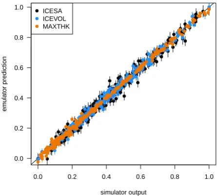
Fig. 3.Leave-one-out cross validation for a Gaussian process emulator, showing good performance in prediction. We exclude a member from the ensemble, and predict the output, given the set of input parameters. We repeat this process across the ensemble, for three summary simulator outputs. Vertical lines represent±1standard deviation.

26

Fig. 3. Leave-one-out cross-validation for a Gaussian process

emu-lator, showing good performance in prediction. We exclude a mem-ber from the ensemble, and predict the output, given the set of input parameters. We repeat this process across the ensemble, for three summary simulator outputs. Vertical lines represent±1 standard de-viation.

are estimated via the posterior mode, as set out by Oakley (1999).

The emulator fits a “best estimate” of the simulator output at a particular input, smoothly through each of the available outputs. It then estimates the uncertainty at each point, with the uncertainty at known simulator runs reducing to zero, and growing with distance from each known point. There is no “nugget” term, and so the emulator is constrained to fit the points where the simulator has been run exactly. We build a separate emulator for each output, individually. Mathemat-ical details of the GP emulator can be found in, e.g. Kennedy and O’Hagan (2001), or Oakley and O’Hagan (2004).

We check the performance of the emulator by performing both a forward, and an inverse leave-one-out cross-validation analysis. Each ensemble member is excluded in turn, and the emulator built on the remaining members of the ensemble. First, we exclude simulator output, and predict it using the most likely value of the emulator uncertainty distribution, given the set of inputs. The prediction plots for the three out-put summaries given in Fig. 3, show that the emulator works well, with small error and no detectable biases, across the ensemble, and for each of the three outputs. Second, we find the implausibilityI of the true held-out input, given the sim-ulator output. We find this to be below the threshold of 3 in all but 3, 1 and 2 ensemble members, for ICEVOL, ICESA and MAXTHK, respectively. In these members, the value of Iis always below 4.

3.2 Results

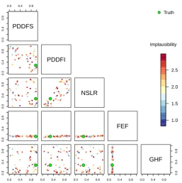
To demonstrate our methods, we first show an example of constraining input parameter space of the (arbitrarily cho-sen) first ensemble member, with no additional observational or simulator discrepancy uncertainty. We show two ways of visualising the constraint of input space in Figs. 4 and 5. Af-ter sampling uniformly from the entire input space, we plot two-dimensional projections of those emulated input points assigned “not implausible” by our method, when we use all three data summaries to constrain the inputs (Fig. 4). It is clear that the true value of the inputs (green point) lies within the region defined by the two dimensional projections. A similar result is obtained looking at the parallel coordinates plot (Fig. 5), showing the full location of the “not implausi-ble” emulated ensemble members (red), along with the tar-get ensemble member (blue). Again, those points calculated as “implausible” are excluded from the plot. It is possible to clearly see how well the input parameter FEF is constrained, using the ensemble data. As each input is plotted over its en-tire range, it is easy to see the “not implausible” range of each parameter in Fig. 5, as the difference between the uppermost and lowermost points on each axis.

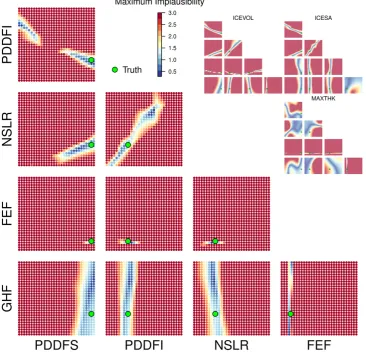
Once we have established that the emulator is accurate to an acceptable degree, its flexibility allows us to conduct many useful analyses that are too expensive to conduct with the original simulator. For example, we can begin to study the behaviour of the simulator, in terms of its individual in-puts. We conduct a “two-at-a-time” sensitivity analysis, and plot the results in Fig. 6. Again, we use the first ensemble member as an example. Each subplot shows the estimated implausibility measure I, when the named inputs are var-ied across a regular grid, and the remaining three inputs are held at their true values. The contributions to the final “max-imum implausibility” measure from each observation type are shown in the inset (top right), and the true values of the ensemble member are plotted as a green point. In this kind of analysis, it quickly becomes clear that “not implausible” regions of input space often form hyperplanes within high dimensional input space.

We use our emulated implausibility method outlined in Sect. 2.4 in order to invert the emulator, and provide a set of metrics for the ensemble members in a leave-one-out fash-ion. We assume that we have no prior information on the pre-cise location of any ensemble member within the input space, and so we use a uniform distribution across the ensemble as a prior distribution. We take a large Monte Carlo sample of inputs and corresponding outputs (order thousands) from the emulator over the entire domain, and find their implausibil-ityI, according to Eq. (3). Using the emulated implausibility, we calculateV andRfor each ensemble member.

(8)

0.0 0.4 0.8

0.0

0.4

0.8

PDDFS

0.0

0.4

0.8

● ●

●

● ●

●

● ●

●

● ●

●

● ● ●

● ●

●

● ●

●

● ●

● ● ● ●

●

● ●

●

● ●

●

PDDFI

0.0

0.4

0.8

●

● ●

●

● ●

●

● ●

●

● ●

●

● ●

●

● ●

●

● ●

●

● ●

●

● ●

●

● ●

● ● ●

●

● ●

●

● ● ●

●

● ●

●

● ●

●

● ●

● ● ●

●

● ●

● ● ●

● ●

●

● ●

●

● ● ●

● ●

● ● ●

● ●

● ● ●

●

● ● ●

● ●

●

NSLR

0.0

0.4

0.8

●●●●

●●●●●●● ●●●● ●●●●

●●●●●●●●●●●●●●●●●●●●●●●●●●●●●●●●●_●●●● ●●●●●●●●●●●●_●●●●●●●●●●●●●●●●●●●●●●●●●●●●●●●●●●●●●●●●●●●● ●●●●●●●●●●●●●●●●●●_●●●●●●●●●●●●●●●●●●●●●●●●●●●●●●●●●●●●●●

FEF

0.0 0.4 0.8

0.0

0.4

0.8

● ●

●

● ● ● ●

●

● ●

●

● ●

● ● ●

● ●

● ● ●

●

● ●

●

● ●

● ● ●

● ●

●

● ●

●

● ●

●● ● ●

0.0 0.4 0.8

● ●

●

● ●

●

● ● ●

●

● ●

●

● ●

●

● ● ●

● ●

● ● ●

● ●

●

● ●

●

● ●

●

0.0 0.4 0.8

● ●

●

● ●

●

● ● ●

●

● ●

●

●● ●

● ●

●

● ●

●

● ●

● ● ●

● ●

●

● ●

●

● ●

●

0.0 0.4 0.8

● ●

●

● ● ●

●

● ●

●●

● ●

● ● ●

● ● ● ● ● ● ●

● ● ●

●

●● ●

● ●

● ● ● ● ●

● ● ●

● ●

●

● ●

●

0.0 0.4 0.8

0.0

0.4

0.8

GHF

● Truth

1.0 1.5 2.0 2.5 Implausibility

Fig. 4.

Two-dimensional projections of emulated “not implausible” (

I <

3 ) ensemble members, when

the true inputs are those of the (arbitrarily chosen) first ensemble member. Implausibility is calculated

as the maximum of that from all three summaries of the output data – ICEVOL, ICESA and MAXTHK.

Emulated implausible members (not shown) are spread evenly through the input space. The true value of

the inputs (the target) is shown as a green point.

27

Fig. 4. Two-dimensional projections of emulated “not implausible” (I <3) ensemble members, when the true inputs are those of the

(ar-bitrarily chosen) first ensemble member. Implausibility is calculated as the maximum of that from all three summaries of the output data – ICEVOL, ICESA and MAXTHK. Emulated implausible members (not shown) are spread evenly through the input space. The true value of the inputs (the target) is shown as a green point.

PDDFS PDDFI NSLR FEF GHF

0 1

"Not Implausible" inputs Target

Fig. 5.Parallel coordinates plot of emulated “not implausible” (I <3) ensemble members (red), when

the true inputs are those of the (arbitrarily chosen) first ensemble member (blue). Lines join points on the y-axis, normalised to the ensemble maxima and minima, with each line representing a point in parameter space. Implausibility is calculated as the maximum of all three summaries of the output data – ICEVOL, ICESA and MAXTHK. Emulated implausible members (not shown) are spread evenly through the input space, and would cover the entire range if shown.

28

Fig. 5. Parallel coordinates plot of emulated “not implausible” (I <

3) ensemble members (red), when the true inputs are those of the (arbitrarily chosen) first ensemble member (blue). Lines join points on theyaxis, normalised to the ensemble maxima and minima, with each line representing a point in parameter space. Implausibility is calculated as the maximum of all three summaries of the output data – ICEVOL, ICESA and MAXTHK. Emulated implausible members (not shown) are spread evenly through the input space, and would cover the entire range if shown.

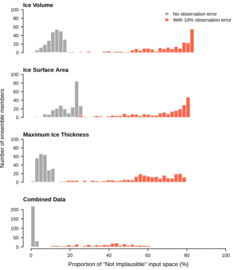
uncertainty, in order to test the sensitivity of our metrics to a real-world situation. We fix the standard deviation of the representative observational error as 10 % of the maximum simulated value for each of the outputs in the ensemble. This uncertainty might also represent a discrepancy uncertainty, as observational and discrepancy uncertainty are added in the denominator in Eq. (3). We test each of our simulator outputs in turn, to find which might provide the most use-ful constraint overall, or for any of the particular simulator inputs.

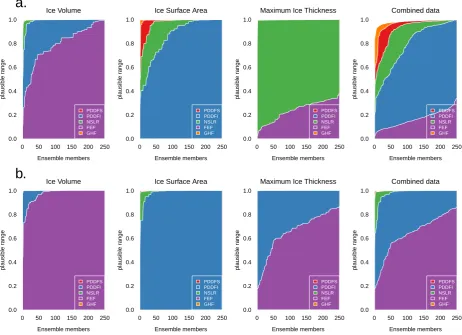
In Fig. 7, we see the distribution across the ensemble of the constraintR– the range of inputs for each input eter that are not implausible. The constraint for each param-eter is represented by the block of colour, reaching a height on they axis. An ensemble member filling the full height is marginally unconstrained by the data; a member reaching halfway up they axis is constrained to 50 % of the range of the original ensemble. The ensemble members are plot-ted along thex axis, ordered from the strongest constrained member to the weakest, independently for each parameter.

Columns of individual plots show the results when sum-marising the simulator outputs in the three different ways, with the final column representing constraint combining all three ways of summarising the data. The top row, (marked a), represents the upper bound of constraint possible – that with no observational or simulator discrepancy uncertainty. The