Volume 33 Issue 3 Article 4
2006
Quantifying Foreseeability
Quantifying Foreseeability
Oren Bar-Gill
Follow this and additional works at: https://ir.law.fsu.edu/lr
Part of the Law Commons
Recommended Citation Recommended Citation
Oren Bar-Gill, Quantifying Foreseeability, 33 Fla. St. U. L. Rev. (2006) .
https://ir.law.fsu.edu/lr/vol33/iss3/4
F
LORIDA
S
TATE
U
NIVERSITY
L
AW
R
EVIEW
Q
UANTIFYING
F
ORESEEABILITY
Oren Bar-Gill
V
OLUME
33
S
PRING
2006
N
UMBER
3
Recommended citation: Oren Bar-Gill, Quantifying Foreseeability, 33 FLA. ST. U. L. REV.
OREN BAR-GILL*
ABSTRACT
This Article extends the law-and-economics literature on the fore-seeability doctrine and on contract default rules more generally. It de-rives (numerically) the optimal default cap on contractual damages in a model with a continuum of buyer types and perfect competition among sellers. When communication costs are low, the optimal cap is significantly higher than the damages incurred by the average buyer. A better performance technology reduces the optimal damages cap. Greater homogeneity among buyers increases the optimal cap. The Ar-ticle identifies conditions under which an optimally defined foresee-ability threshold significantly increases welfare. It also explores the normative implications of the doctrinal preclusion of a zero-damages default.
I. INTRODUCTION... 620
II. MODEL... 624
A. Framework of Analysis... 624
B. The Buyer’s Decision Whether to Disclose Her Type... 625
1. The Four-Region Equilibrium... 625
2. The Three-Region Equilibrium... 627
C. The Welfare Maximizing Rule... 627
D. Numeric Analysis... 627
III. THE OPTIMAL DAMAGES CAP... 628
A. Communication Costs... 629
B. Performance Technology... 631
C. Distribution of Buyer Valuations... 635
IV. HOW IMPORTANT IS IT TO OPTIMALLY SET THE FORESEEABILITY THRESHOLD? ... 639
V. AZERO-DAMAGES DEFAULT... 642
VI. EXTENSIONS... 647
VII. CONCLUSION... 648
I. INTRODUCTION
Contract law limits recovery for breach of contract. In particular, harm deemed extraordinary or excessively remote is excluded from the damages measure under the foreseeability doctrine.1 Limited
re-covery is not, however, an immutable tenet of contract law. It is a de-fault rule. A contracting party can render an extraordinary harm re-coverable simply by informing the other party that such harm is pos-sible in the present case. The foreseeability doctrine in effect speci-fies a threshold level of harm. Harm below the threshold, ordinary harm, is always recoverable. Harm above the threshold is recover-able only if it is communicated to the other party at the time of con-tracting. What is the optimal threshold? What harm should be recov-erable by default, and when should specific communication be re-quired?
The foreseeability doctrine has served in the law-and-economics literature as the primary example for studying the optimal design of default rules.2 I too hope that the analysis developed in this Article
will be modestly informative for general default rule theory. I do not, however, develop these broader implications here. Rather, I focus solely on foreseeability doctrine. My goal is to derive the optimal de-fault cap on contract damages and to explore the relationship be-tween this theoretical optimum and the judicial elucidation of the foreseeability doctrine.
The analysis is motivated by the recognition that damages for breach of contract lie on a continuum—from the obvious harm that would always follow a breach of the type of contract considered to the most remote and extraordinary harm that would occur in only a very small percentage of cases. It is this continuum that foreseeability doctrine divides—into recoverable and nonrecoverable damages—by setting a cap, a threshold level of damages. The question I ask is thus somewhat different from the standard question in this literature. Most previous accounts assume two discrete levels of damages—low damages and high damages—and ask whether the default rule should allow recovery for only low damages (limited liability), or for both low and high damages (unlimited liability). Rather than asking
whether liability for breach of contract should be limited or unlim-ited, I ask where on the continuum of damages levels the limit should be placed.3
The first step in the analysis is to derive the equilibrium behavior of the contracting parties. There are two alternative equilibria identi-fied by the number of regions into which the group of buyers is di-vided. In the first, four-region equilibrium, buyers divide into four groups: (1) buyers with low valuations (and correspondingly low damages) who choose not to contract because they do not want to pay the high pooling price and they do not find it worthwhile to expend communication costs in order to attain a lower price, (2) buyers with higher valuations who separate themselves in order to pay a lower price, (3) buyers with intermediate valuations who save on communi-cation costs and pay the pooling price, and (4) buyers with high valuations who are willing to pay a higher price to guarantee their expectation interest. In the second, three-region equilibrium, buyers divide into only three groups: (1) buyers with low valuations who choose not to contract, (2) buyers with intermediate valuations who save on communication costs and pay the pooling price, and (3) buy-ers with high valuations who are willing to pay a higher price to guarantee their expectation interest.
The size of the different groups in both equilibria depends on the damages cap. What is the optimal cap? In the standard two-type model, the optimal rule—that is, the optimal choice between limited and unlimited liability—induces the right type of equilibrium (pool-ing or separat(pool-ing) and, if separation is efficient, guarantees that this separation is attained with minimum communication costs.4 In the
continuous-type model, characterizing the optimal rule is more com-plicated. First, as mentioned above, the choice is no longer binary— limited versus unlimited liability; rather the optimal cap can be anywhere on the continuum of possible damages levels. Second, the pooling versus separating question is no longer a binary question. There are different degrees of pooling and separating.
3. Bebchuk and Shavell briefly consider a continuous-type extension to their two-type model. See Bebchuk & Shavell, supra note 2, at 308.Johnston studies a continuous-type model but considers only two possible rules: an unlimited liability rule and a limited liability rule with liability capped at the average level of damages. See Johnston, supra
note 2, at 626-27, 651. Moreover, Johnston assumes that sellers have market power, while I assume perfect competition among sellers. Seeid. at 636-37. Geis uses a continuous-type model but assumes discrete care levels (and, correspondingly, discrete probabilities of per-formance) and considers only an unlimited liability rule and a limited liability rule defined by a fixed damages cap. See Geis, supra note 2. Adler studies a two-type model but charac-terizes each buyer type by a stochastic continuous distribution of damages. See Adler, su-pra note 2, at 1561.
Finally, the continuous-type model reveals an efficiency consid-eration that the two-type models, at least those assuming perfect competition, do not emphasize: a potentially significant group of buy-ers might be driven out of the market. It is well recognized that a seller with market power may choose not to serve the low end of the market.5 The continuous-type model shows that low-valuation buyers
might leave the market even with perfect competition among sellers. And this inefficiency must also be considered in setting the optimal damages cap.6
The optimal damages cap achieves the right balance of pooling and separation, minimizes communication costs, and optimally con-trols the entry and exit of low-valuation buyers. I develop a numeric algorithm that solves for the optimal cap and study how different pa-rameters, specifically the magnitude of communication costs, the per-formance technology, and the distribution of buyer valuations, affect the optimal cap.
The analysis yields the following results. When communication costs are low, as is arguably the case in most contracting environ-ments, the optimal damages cap is significantly above the average buyer valuation.7 In fact, for a broad range of parameter values the
optimal cap is above the eightieth percentile of buyer valuations. The optimal damages cap is lower when communication costs are larger, but even when communication costs are very large, the optimal fore-seeability threshold significantly exceeds the average buyer valua-tion. This result supports the modern tendency to narrowly apply the foreseeability requirement.8
The performance technology, and specifically the cost-effectiveness of reducing the probability of breach, also has a signifi-cant effect on the optimal damages cap. Focusing on the more com-mon, low communication costs environments, a superior performance technology requires a lower foreseeability threshold—a counterintui-tive result. It is noteworthy that even this lower cap is significantly above the average buyer valuation. The remaining parameter is the
5. See, e.g., Ayres & Gertner, Strategic Contractual Inefficiency, supra note 2, at 744, 747. 6. Barry Adler notes that marginal buyers might be driven out of the market. Adler,
supra note 2, at 1556 n.25. Adler, however, blames this result on the high pooling price that results under expansive liability. Id. at 1556-57. As I argue below, low-valuation buy-ers might leave the market because they do not find it worthwhile to secure a low price by communicating their type.
distribution of buyer valuations. The numeric analysis suggests that a higher foreseeability threshold should be set when the distribution of buyer valuations is more homogeneous. The implications of asym-metric/skewed distributions of buyer valuations are also briefly ex-plored.
How important is it to optimally set the foreseeability threshold? How much welfare will be lost if the wrong default is chosen? Not surprisingly, if communication costs are sufficiently small, the legal default matters very little. The analytical framework developed in this Article can tell us how small is sufficiently small. For example, if losing 1% of the maximum attainable welfare is considered to be in-sufficiently important in a given context, then as long as communica-tion costs do not exceed 2% of the average buyer valuacommunica-tion, even sig-nificant deviations from the optimal default should not raise concern. The optimal foreseeability threshold described above is in some cases only a second-best optimum. The optimization problem that produced this threshold was solved under the constraint that dam-ages cannot be capped too close to zero. The numeric algorithm thus ruled out a zero- (or close to zero) damages default, even when such a default produced the highest welfare. This doctrinal-institutional constraint reflects the view that courts would resist a regime of no li-ability for breach of contract, even if this is only a default regime.9
What are the welfare implications of the doctrinal constraint? When communication costs are high, the constraint is not binding. In most real-world environments, however, where communication costs are low, the doctrinal constraint is binding. Moreover, the welfare loss incurred by ruling out a zero-damages default can be quite sig-nificant—up to 10% of the maximum attainable welfare for some pa-rameter values. These adverse welfare implications merit a reconsid-eration of the doctrine behind the doctrinal constraint. While a broad “no damages” default seems institutionally untenable, zero-damages defaults for specific categories of damages, for example, lost retail profits or consequential damages more generally, does not seem un-thinkable.10
9. Robert Scott and George Triantis, while developing a powerful case against the compensation principle in contract law, recognize that “[t]he dominance of the compensa-tion principle is now unquescompensa-tioned.” Robert E. Scott & George G. Triantis, Embedded Op-tions and the Case Against Compensation in Contract Law, 104 COLUM.L.REV. 1428, 1446 (2004).
The analysis in this Article builds upon and extends previous work on the foreseeability doctrine. This line of research suffers from an important limitation. The theoretical results and specifically the optimal damages cap depend on parameter values that are difficult to ascertain empirically.11 The practical value of this line of research
depends on the ability to import—from other social sciences—and utilize more sophisticated empirical tools.12 It is important to
empha-size that the empirical assessments required to operationalize the theoretical results need not be absolutely accurate. The analysis in this Article suggests that even rough estimates of the underlying pa-rameters can lead to a better calibration of the foreseeability thresh-old and thus to greater welfare.
From a policy perspective the parameter that is most important to evaluate empirically is the magnitude of communication costs. The model developed in this Article can tell us how large communication costs must be for the default rule to matter. But only empirical re-search can identify the contractual environments where communica-tion costs are sufficiently large to justify an effort to optimally set the default.
The remainder of the Article is organized as follows. Part II devel-ops the continuous-type model. Part III reports the results of the numeric analysis: how the optimal damages cap depends on the un-derlying parameters. Part IV identifies conditions under which an optimally defined foreseeability threshold can significantly increase welfare. Part V explores the normative implications of the doctrinal constraint that precludes a zero-damages default. Part VI discusses extensions. Part VII concludes.
II. MODEL
A. Framework of Analysis
A seller operating in a perfectly competitive market faces a buyer whose valuation of the offered product or service is unknown to the seller. Let v denote the value of the product or service—the value of contractual performance—to the buyer. This value, v, is the buyer’s type. The seller knows only the distribution of buyer valuations, f(v). The support of f(v) is normalized to [0,1] without loss of generality. For any specific buyer, the value of performance is private
edy. The difficulty, of course, is that the distinction between regular and consequential damages is not always easy to draw.
11. See Adler, supra note 2; Eric A. Posner, Economic Analysis of Contract Law After Three Decades: Success or Failure?, 112 YALE L.J. 829 (2003).
tion, but the buyer can communicate her valuation to the seller at a cost, k.
The probability of successful performance is given by p(x), where x represents the seller’s precautions (in monetary terms). I assume that p′(x) > 0 and p′′(x) < 0 (and, of course, p(x)
∈
[0,1]). If the seller breaches the contract, he will pay damages, d. The damage measure can take one of two values: (1) the actual full expectation measure, v, or (2) the legally determined foreseeable harm damage measure, vˆ .13Let d(v) denote the damage measure applicable to buyer v.
The seller’s expected total cost when facing a subset of buyers
[ ]
vvv∈ , is =v∫
[
(
−)
⋅ +]
v v
v x px dv x f vdv
c ( ) 1 ( ) ( ) ( ) .14 The seller will choose x to minimize his expected cost. The minimized cost, cvv(x*)≡cvv, de-fines the price charged by the seller. The profit of buyer v is
(
p x)
dv cvvv x p
v)= ( )⋅ + − ( ) ⋅ ( )−
( 1
π (minus communication costs, k, when the buyer chooses to communicate her type to the seller).
B. The Buyer’s Decision Whether to Disclose Her Type
There are two alternative equilibria in this model. In the first, four-region equilibrium buyers divide into four sub-groups: (1) buyers with low valuations, v
∈
[0, v1], who choose not to contract because they do not want to pay the high pooling price and they do not find it worthwhile to expend k in order to attain a lower price, (2) buyers with higher valuations, v∈
[v1, v2], who separate themselves in order to pay a lower price, (3) buyers with intermediate valuations, v∈
[v2,v3], who save on communication costs and pay the pooling price, and (4) buyers with high valuations, v
∈
[v3, 1], who are willing to pay a higher price to guarantee their expectation interest. In the second, three-region equilibrium, buyers divide into only three sub-groups: (1) buyers with low valuations, v∈
[0, v1], who choose not to contract, (2) buyers with intermediate valuations, v∈
[v2, v3], who save on communication costs and pay the pooling price, and (3) buyers with high valuations, v∈
[v3, 1], who are willing to pay a higher price to guarantee their expectation interest.1. The Four-Region Equilibrium
The threshold value v1 can be found by solving (1) v1 =cv1+k.
13. I abstract from the possibility of stipulated damages set at a level other than the full expectation measure.
The marginal buyer is indifferent between exiting the market and earning a zero payoff on the one hand, and communicating her type and earning her valuation minus the tailored price (and minus com-munication costs) on the other hand. The threshold price is
(
( *( )))
*( )1 1 1
1 1 px v v x v
cv = − ⋅ + , where *( ) argmin
(
( ( )))
( )1 1 1
1 1 px v v xv
v
x = − ⋅ + .
The threshold value v2 satisfies
(
)
2 23 22
2 cv k p x v 1 px v cvv
v − − = ( )⋅ + − ( ) ⋅ − , or (2) cv2+k=cv2v3.
The marginal buyer is indifferent between paying the tailored price plus communication costs on the one hand, and paying the higher pooling price on the other hand. Note that v2 <vˆ. A buyer with v2 =vˆ−ε would not expend k to get a marginally more favor-able combination of price and care. The threshold price is
(
( *( )))
*( )2 2 2
2 1 px v v x v
cv = − ⋅ + ,where *( ) argmin
(
( ( )))
( )2 2 2
2 1 pxv v xv
v
x = − ⋅ + .
A seller facing a pool of buyers with v∈[v2,v3] expects a total cost of
[ ]
(
) (
⋅∫[
−)
⋅ +]
∈ = 3 2 3 2 1 1 3 2 v v vv x v v v p x dv x f v dv
c ( ) ( ) ( )
, Pr )
( , where
> ≤ = v v v v v v v d ˆ , ˆ ˆ , )
( , or
[ ]
(
) (
[
)
]
[
(
)
]
∫ − ⋅ + +∫ − ⋅ + ⋅ ∈ = 3 2 32 1 1
1 3 2 v v v v v
v x v v v px v x f vdv px v x f vdv
c ˆ ˆ ) ( ˆ ) ( ) ( ) ( , Pr ) ( .
The pooling level of precaution is xvv argmin cvv (x)
3 2 3
2 = , and the
pooling price is cv2v3 ≡cv2v3(xv2v3). The threshold value v3 satisfies
(
p x)
v c v c k vx
p( )⋅ 3+ 1− ( ) ⋅ˆ− v2v3 = 3− v3− , or
(3)
(
1−p(x)) (
⋅ v3−vˆ)
=(
cv3−cv2v3)
+k.The marginal buyer is indifferent between paying the pooling price and getting only the legally determined damages measure in case of breach on the one hand, and paying the higher tailored price plus communica-tion costs to guarantee her expectacommunica-tion interest on the other. Note that
v
v3 > ˆ. A buyer with v3 =vˆ+ε would not expend k to get a marginally
more favorable combination of price and care. The threshold price is
(
( *( )))
*( )3 3 3
1
3 px v v x v
cv = − ⋅ + , where *( ) argmin
(
( ( )))
( ) 3 3 33 1 p xv v xv
v
x = − ⋅ + .
Using equations (1) through (3), I can solve for the threshold values, v1,
2
v and v3, as a function of the legally determined damages cap, vˆ . The
FIGURE 1
THE FOUR-REGION EQUILIBRIUM
2. The Three-Region Equilibrium
The threshold value v2 satisfies 0=p(x)⋅v2+
(
1−p(x))
⋅v2−cv2v3, or(4)
3 2
2 cvv
v = .
The marginal buyer is indifferent between exiting the market and earning a zero payoff on the one hand, and paying the pooling price on the other hand. The threshold value v3 is derived from equation (3), as in the four-region equilibrium.
Using equations (3) and (4), I can solve for the threshold values,
2
v and v3, as a function of the legally determined damages cap, vˆ . The three-region equilibrium is depicted in Figure 2.
FIGURE 2
THE THREE-REGION EQUILIBRIUM
C. The Welfare Maximizing Rule
For any legally determined damages cap, vˆ , there is a unique vec-tor of threshold values—(v1,v2,v3) in the four-region equilibrium, and (v2,v3) in the three-region equilibrium—that defines the sub-groups of buyers and implicitly the price, cvv, paid by each buyer and
the profit, π(v), enjoyed by each buyer. Social welfare is given by dv
v f v v
W(ˆ)=∫1 ( ) ( )
0
π . The optimal vˆ solves max (ˆ)
ˆ W v
v .
D. Numeric Analysis
com-plexity. Solving the continuous-type model analytically is beyond this author’s capabilities. I therefore resort to numeric analysis, solving the model (or, more precisely, asking a computer to solve the model) for different parameter values.15
First and foremost, I study the effects of communication costs by varying the magnitude of the parameter k. Second, I study the impli-cations of different performance technologies. I use the probability of performance function p x = −e−λx
1
)
( , where the λ parameter repre-sents the performance technology, specifically the efficacy of precau-tion expenditures in reducing the probability of breach.
Finally, I study the role of the distribution of buyer valuations. The distribution of buyer valuations is assumed to follow a Beta dis-tribution. The Beta distribution has a domain of [0, 1].16 The
distribu-tion’s two parameters, A and B, determine the variance and skew-ness of the distribution. The benchmark distribution in this study is a Beta distribution with parameter values A = B = 1, which is a Uni-form distribution. The implications of greater homogeneity among buyers is explored by increasing the values of the distribution pa-rameters while maintaining A = B. Removing the A = B constraint al-lows me to explore the implications of skewed distributions.
The broad range of parameters studied represents many real-life contracting scenarios. Nevertheless, it should be recognized that the generality of the results is limited by the specific functional forms used in the numeric analysis. A different performance technology or a different distribution of buyer valuations will clearly affect the quantitative results. Still, many of the qualitative insights derived from the numeric analysis are robust to variations in the assumed functional forms. Moreover, the general framework developed in this Article can be used to reassess the quantitative results for alterna-tive functional forms.
III. THE OPTIMAL DAMAGES CAP
The model developed in Part II can be used to study the character-istics of the optimal damages cap. How do different parameters— specifically the magnitude of communication costs—the performance technology, and the distribution of buyer valuations affect the opti-mal cap?
15. The numeric solutions were derived using Matlab (Version 7).
A. Communication Costs
The magnitude of communication costs, as captured by the k
pa-rameter, significantly affects the optimal damages cap, vˆ . Figure 3
depicts the functional relationship between vˆ and k, when buyer
valuations are uniformly distributed and the performance technology
is characterized by
λ
=
5
. Figure 3 also depicts the threshold values,v1, v2,and v3, as a function of k.
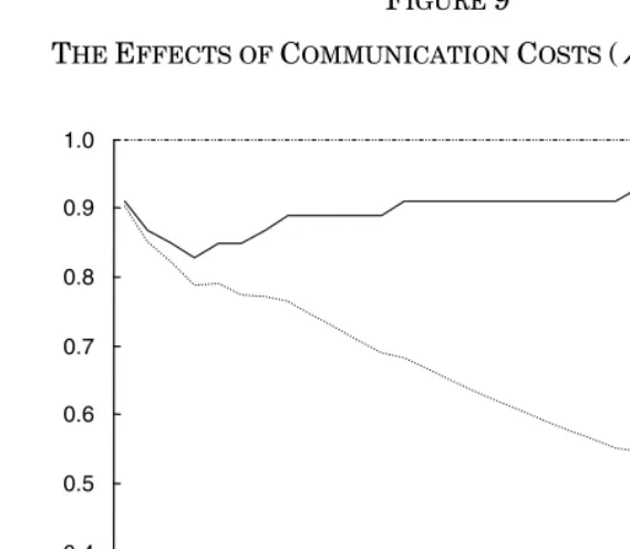
FIGURE 3
THE EFFECTS OF COMMUNICATION COSTS (
λ
=
5
,A=B= 1)Starting at the low communication costs end of the scale, the op-timal foreseeability threshold is relatively high, at the ninetieth per-centile of possible valuations of contractual performance. An increase in communication costs leads to a decline in the optimal damages cap. The reduced pooling price achieved by the lower cap allows more
low-value buyers to join the pool and save on communication costs: v2
decreases. The optimal cap falls monotonically, further increasing the size of the pool, and saving on communication costs.
It is not until communication costs reach a fairly high level—14%
of the average buyer valuation—that the decreasing v2 graph
inter-sects with the increasing v1 graph and the four-region equilibrium
gives way to the three-region equilibrium (not depicted in Figure 3). At this point there is no more communication by low-value buyers:
0 0.01 0.02 0.03 0.04 0.05 0.06
0.2 0.3 0.4 0.5 0.6 0.7 0.8 0.9 1.0
k
opt vˆ
1
v
they either join the pool or exit (the communication option is always dominated by at least one of these two alternatives). Switching from the four-region equilibrium to the three-region equilibrium generates a discontinuity in the level of the optimal damages cap.
As communication costs continue to increase, the optimal cap re-sumes its monotonic decline. This decline lowers the pooling price and induces more low-value buyers to enter the market. At this stage communication costs are not borne by anyone. Still, higher communi-cation costs prevent higher-value buyers from leaving the pool (even when the damages cap falls) and, thus, facilitate the inclusion of more low-value buyers through a reduced pooling price brought about by a lower damages cap.
FIGURE 4
WELFARE AS A FUNCTION OF COMMUNICATION COSTS
(
λ
=
5
,A=B=1)Starting from very low communication costs, an increase in com-munication costs from 0.001, or 0.2% of the average buyer valuation, to 0.01, or 2% of the average buyer valuation, leads to a 5.3% reduc-tion in welfare. The marginal effect of communicareduc-tion costs on wel-fare decreases as communication costs increase. In fact, for suffi-ciently high communication costs, specifically k = 0.05, or 10% of the average buyer valuation, an increase in communication costs in-creases welfare. A possible explanation is that the high communica-tion costs are not incurred by buyers, but rather serve to support an efficient pooling equilibrium that minimizes communication costs.
B. Performance Technology
Are the results stated in Part III.A robust to changes in the per-formance technology? I begin by studying more efficient perper-formance technologies. For concreteness, compare the performance technology studied in Part III.A, which is characterized by
λ
=
5
, and a moreef-ficient performance technology characterized by
λ
=
10
. Figure 5replicates Figure 3 with a
λ
=
10
technology.0 0.01 0.02 0.03 0.04 0.05 0.06
0.144 0.146 0.148 0.150
0.152 0.154 0.156 0.158 0.160
k W
FIGURE 5
THE EFFECTS OF COMMUNICATION COSTS (
λ
=
10
,A=B=1)When communication costs are k = 0.001, the optimal foreseeabil-ity threshold given the
λ
=
5
technology is at the ninetiethpercen-tile of possible buyer valuations. With the more efficient
λ
=
10
technology, the optimal threshold is below the ninetieth percentile. The more efficient technology makes pooling more attractive to high-valuation buyers. It is thus possible to reduce the foreseeability threshold, increase the size of the pool, and lower communication costs without driving high-valuation buyers out of the pool. The size of the pool increases further, compared to the size of the pool with the
λ
=
5
technology, as communication costs rise. The optimalfore-seeability threshold with a
λ
=
10
technology is always lower thanthe optimal threshold with a
λ
=
5
technology. These results arede-picted in Figure 6.
0 0.01 0.02 0.03 0.04 0.05 0.06
0.1 0.2 0.3 0.4 0.5 0.6 0.7 0.8 0.9 1.0
k
opt vˆ
1
v2 v
3
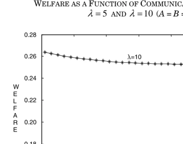
FIGURE 6
*
ˆ
v AS A FUNCTION OF k FOR
λ
=
5
ANDλ
=
10
The more efficient performance technology also significantly re-duces the number of low-valuation buyers who withdraw from the market. Specifically, for communication costs of k = 0.001 only 12% of all buyers withdraw from the market with the
λ
=
10
technology, ascompared to over 20% of all buyers who withdraw from the market with the
λ
=
5
technology.Not surprisingly, the more efficient performance technology pro-duces higher welfare at every level of communication costs. Figure 7 graphs welfare as a function of communication costs for both the
5
=
λ
technology and theλ
=
10
technology.0 0.01 0.02 0.03 0.04 0.05 0.06
0.65 0.75 0.85 0.95 1.00
k opt vˆ
λ =10 0.70
0.80 0.90
FIGURE 7
WELFARE AS A FUNCTION OF COMMUNICATION COSTS FOR
5
=
λ
ANDλ
=
10
(A=B=1)The welfare effects are quite large: moving from a
λ
=
5
performancetechnology to a
λ
=
10
performance technology entails a welfarein-crease of over 60%.
The comparison between the
λ
=
5
technology and theλ
=
10
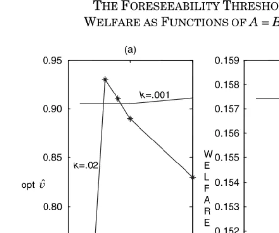
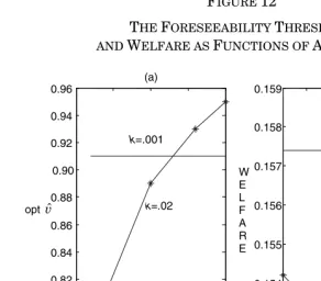
technology demonstrates the impact of the performance technology on both the optimal foreseeability threshold and the attainable level of welfare. Figure 8 presents a broader comparative statics analysis. Figure 8(a) plots the optimal threshold as a function of the perform-ance technology (
λ
∈
[1, 50]) for k = 0.001 and k = 0.02. Figure 8(b) plots the maximum attainable social welfare as a function of the per-formance technology (λ
∈
[1, 50]) for k = 0.001 and k = 0.02.0 0.01 0.02 0.03 0.04 0.05 0.06
0.16 0.18 0.22 0.24 0.26 0.28
k
λ =5
λ=10
FIGURE 8
THE FORESEEABILITY THRESHOLD AND
WELFARE AS FUNCTIONS OF
λ
(A=B=1)C. Distribution of Buyer Valuations
Another important factor affecting the optimal damages cap is the distribution of buyer valuations. Recall that with heterogeneous buy-ers, specifically with buyer valuations following a Uniform distribu-tion, for very low communication costs the optimal threshold was ap-proximately 0.90. And when communication costs increased, the op-timal threshold declined monotonically.17 As buyers become more
homogeneous, these results change. First, the initial decrease in the optimal threshold when communication costs increase is smaller. Second, after a certain level of communication costs is reached, this decrease is reversed, and the optimal foreseeability threshold in-creases with communication costs. The level of communication costs at which this change in trajectory occurs is decreasing in the degree of homogeneity among buyers.
These results are demonstrated for a distribution of buyers char-acterized by A = B = 5 in Figure 9.
17. Only at a very high level of communication costs, k = 0.05, and at a relatively low foreseeability threshold, approximately 0.63, did the trajectory change and the optimal threshold began to increase as communication costs rose further. The reason for this change in trajectory was the switch from the four- to the three-region equilibrium.
0 20 40 60
0.65 0.75 0.85 0.95 1.00
(a)
0 20 40 60
0.15 0.35 0.45
(b)
k=.001
k=.02 k=.001
k=.02 0.70
0.80 0.90
0.10 0.20 0.25 0.30 0.40 0.50
W E L F A R E opt vˆ
FIGURE 9
THE EFFECTS OF COMMUNICATION COSTS (
λ
=
5
,A=B=5)Overall, the foreseeability thresholds are higher when the distri-bution of buyer valuations is more homogeneous. Moreover, the abso-lute thresholds underestimate the impact of increased homogeneity. With a uniform distribution of buyer valuations, a 0.9 foreseeability threshold implies that 90% of buyers would be fully compensated (for damages from breach of contract) under the default. With the more homogeneous A = B = 5 distribution, a 0.9 foreseeability threshold implies that over 99% of buyers would be fully compensated for breach of contract under the default.
What are the welfare implications of the degree of homogeneity? Figure 10 plots welfare as a function of communication costs for both A = B = 1 and A = B = 5.
0 0.01 0.02 0.03 0.04 0.05 0.06
0.2 0.3 0.4 0.5 0.6 0.7 0.8 0.9 1.0
opt vˆ
1
v
3
v
k
2
FIGURE 10
WELFARE AS A FUNCTION OF k
FOR A = B = 1 AND A = B = 5 (
λ
=
5
)Figure 11 presents a broader comparative statistical analysis. Figure 11(a) plots the optimal threshold as a function of the degree of
homogeneity (A = B
∈
[1,2,3,4,5,10]) for k = 0.001 and k = 0.02.Fig-ure 11(b) plots the maximum attainable social welfare as a function
of the degree of homogeneity (A = B
∈
[1,2,3,4,5,10]) for k = 0.001 andk = 0.02.
0 0.01 0.02 0.03 0.04 0.05 0.06
0.145 0.155 0.165
k
A=B=5
A=B=1
W E L F A R E 0.150
FIGURE 11
THE FORESEEABILITY THRESHOLD AND
WELFARE AS FUNCTIONS OF A=B(
λ
=
5
)The analysis thus far focused on symmetric distributions of buyer valuations. How would the results change with skewed distributions? Figure 12 begins to answer this question. It plots the optimal thresh-old (Figure 12(a)) and social welfare (Figure 12(b)) as a function of the ratio A/B, where a ratio A/B < 1 represents a distribution that is skewed to the left and a ratio A/B > 1 represents a distribution that is skewed to the right.
0 5 10
0.75 0.85 0.95
A=B (a)
0 5 10
0.149 0.151 0.152 0.153 0.154 0.155 0.156 0.157 0.158 0.159
A=B (b)
k=.001
k=.02
k=.001
k=.02
0.70 0.80 0.90
FIGURE 12
THE FORESEEABILITY THRESHOLD AND WELFARE AS FUNCTIONS OF A/B(
λ
=
5
)IV. HOW IMPORTANT IS IT TO OPTIMALLY SET THE FORESEEABILITY
THRESHOLD?
In many contractual environments communication costs are low. If it is easy to opt out of the default rule, then it should not matter very much whether the default is set optimally.18 Part IV attempts to
quantify this observation. Exactly how much welfare is lost when the default rule is not set optimally? How small must communication costs be to render the choice of default immaterial?
I begin by defining the efficiency cost of a default rule vˆ that de-viates from the optimal default vˆ* as EC
( )
vˆ;vˆ* =[
W( )
vˆ* −W( )
vˆ]
W( )
vˆ* .Figure 13(a) plots EC
( )
v;ˆvˆ* for ˆ [ . ,]1 2 0
∈
v when λ=5, A=B=1, and
k = 0.005. Figure 13(b) plots EC
( )
v;ˆvˆ* for ˆ [ . ,]1 2 0
∈
v when λ=5, 1
= =B
A , and k=0.05.19
18. Recall the perfect competition assumption. In imperfectly competitive markets de-fault rules can significantly affect welfare even when communication costs are very small.
See, e.g., Ayres & Gertner, Strategic Contractual Inefficiency, supra note 2.
19. For an explanation why the domain in Figure 13 is vˆ∈[0.2,1], rather than ]
, [ ˆ∈01
v , see infra Part V (and specifically footnote 21).
0 0.5 1 1.5 2
0.76 0.78 0.82 0.84 0.86 0.88 0.92 0.94 0.96
A/B (A=1,2,5,8,10; B=5) (a)
0.5 1 1.5 2
0.152 0.153 0.154 0.155 0.156 0.157 0.158 0.159 (b)
A/B(A=1,2,5,8,10; B=5) k=.001 k=.02 k=.001 k=.02 W E L F A R E opt vˆ
FIGURE 13
EFFICIENCY COST AS A FUNCTION OF vˆ FOR k = 0.005 AND k = 0.05 (
λ
=
5
, A = B = 1)0.2 0.3 0.4 0.5 0.6 0.7 0.8 0.9 1
0.00 0.02 0.04 0.06 0.08 0.12 0.14 0.16
vˆ
(b)
0.10
0.2 0.3 0.4 0.5 0.6 0.7 0.8 0.9 1
0.0 0.5 1.5 2.5 3.5 4.5
5.0
vˆ
(a)
1.0 2.0 3.0 4.0
EC(vˆ) x 10-3
To facilitate a broader comparative statistical analysis, I use a more specific definition of efficiency costs. I calculate EC
(
vˆ= . ⋅vˆ*)
5 0
and EC
(
vˆ= . ⋅vˆ*)
5
1 , and define
( )
vˆ* max EC(
vˆ . vˆ*) (
,ECvˆ . vˆ*)
EC = =05⋅ =15⋅ as the efficiency cost of
failing to accurately set the default rule at the optimal level vˆ*. This
definition allows me to study how the different parameters affect the magnitude of the efficiency cost generated by inaccurate defaults.20
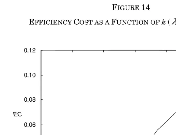
I begin by studying the implications of communication costs. Fig-ure 14 plots EC
( )
vˆ* as a function of k.FIGURE 14
EFFICIENCY COST AS A FUNCTION OF k(
λ
=
5
, A = B = 1)Figure 14 answers the question how small must communication costs be to render the choice of default immaterial. When communication costs are substantial, around 10% of the average buyer valuation, the efficiency cost of choosing the wrong foreseeability threshold is also substantial; almost 10% of the maximum attainable welfare is lost. But even for more reasonable levels of communication costs, say 2%
20. The assumption here is that the court gets the default wrong, but the parties an-ticipate this wrong default rule ex ante. The alternative assumption that ex ante the par-ties are uncertain about the default is discussed in Part VI infra.
0 0.01 0.02 0.03 0.04 0.05 0.06
0.00 0.02 0.04 0.06 0.08 0.12
k EC
of the average buyer valuation, the efficiency cost is nonnegligible, almost 1%.
The magnitude of the communication costs also determines the importance of tailoring the default to the performance technology and to the distribution of buyer valuations. When communication costs are high, such tailoring produces significant welfare gains. When communication costs are small, even large deviations from the optimally tailored default result in an insignificant welfare loss.
V. AZERO-DAMAGES DEFAULT
The optimal foreseeability thresholds derived above were not al-ways optimal. For some parameter values, a very different default rule—a zero-damages default—would produce greater welfare. In other words, the foreseeability thresholds studied thus far were in some instances only second-best optimal, namely, optimal given a feasibility constraint imposed on the optimization problem. The im-posed feasibility constraint is doctrinal or even institutional in na-ture. It posits that courts cannot set a zero-foreseeability threshold.21
This would mean that absent a specific contractual provision to the contrary, there would be no liability for breach of contract.22
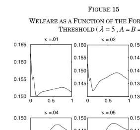
To understand the potential importance of the doctrinal con-straint, it is useful to study the relationship between social welfare and the foreseeability threshold for different levels of communication costs. Figure 15 depicts welfare as a function of the foreseeability threshold for k = 0.1, 0.2, 0.3, 0.4, 0.5 and 0.6, assuming
λ
=
5
and A = B = 1.
21. Since the second-best optimal thresholds studied above are in some cases outper-formed not only by the zero-damages default, but by a range of foreseeability thresholds between zero and 0.2, the imposed doctrinal constraint is more accurately defined as ruling out foreseeability thresholds below one-half of the average buyer valuation.
FIGURE 15
WELFARE AS A FUNCTION OF THE FORESEEABILITY
THRESHOLD (
λ
=
5
,A=B=1)Figure 15 shows that the welfare function has two local maxima: one at a foreseeability threshold above the average valuation (0.5) and another at a foreseeability threshold of zero. The intuition for this bimodal distribution is as follows. A three-region equilibrium is obtained when the foreseeability threshold is sufficiently low (see Figure 2, supra). Low-valuation buyers either withdraw from the market or join the pool. When the foreseeability threshold ap-proaches zero, most of the low-valuation buyers remain in the mar-ket. Moreover, these low-valuation buyers do not incur communica-tion costs. The reduccommunica-tion in communicacommunica-tion costs incurred by low-valuation buyers is, however, counteracted by the increased commu-nication costs incurred by high-valuation buyers. On balance, a fore-seeability threshold near zero produces relatively high welfare, espe-cially when communication costs are low such that the inclusion of low-valuation buyers is the dominant consideration.
When the foreseeability threshold increases from zero, welfare ini-tially falls as more low-value buyers exit the market. When the fore-seeability threshold increases further, the marginal impact of the ex-clusion effect becomes weaker, since the remaining low-value buyers are not easily driven out of the market by a slight increase in the pooling price. Now welfare increases with the foreseeability thresh-old, as this increase economizes on communication costs. At some
0 0.5 1
0.155 0.165
k =.01
0 0.5 1
0.145 0.155
k =.02
0 0.5 1
0.135 0.145
k=.03
0 0.5 1
k =.04
0 0.5 1
k =.05
0 0.5 1
point, the three-region equilibrium is replaced by the four-region equilibrium (see Figure 1, supra). Welfare continues to increase with the foreseeability threshold as long as the marginal communication costs saved by the high-valuation buyers outweigh the marginal communication costs incurred by the low-valuation buyers. When the toll on low-valuation buyers surpasses the benefit to high-valuation buyers, welfare starts to fall and continues to decline monotonically as the foreseeability threshold continues to rise.
Given the bimodal nature of the welfare function, when is the doc-trinal constraint binding? When communication costs are large, the local maximum with a foreseeability threshold above the average buyer valuation is also the global maximum, and the doctrinal con-straint is not binding. When communication costs are small, the local maximum with the zero-foreseeability threshold is the global maxi-mum. Here the doctrinal constraint is binding.
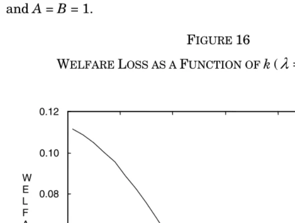
How big are the welfare costs imposed by the doctrinal constraint? Figure 16 plots the welfare loss, as a percentage of the maximum welfare attainable, as a function of communication costs for
λ
=
5
and A = B = 1.
FIGURE 16
WELFARE LOSS AS A FUNCTION OF k(
λ
=
5
,A=B=1)There is no welfare loss when communication costs exceed 0.031. When communication costs drop below 0.031, the doctrinal constraint
0 0.01 0.02 0.03 0.04 0.05 0.06
0.00 0.02 0.04 0.06 0.08 0.12
k 0.10
W E L F A R E
L
kicks in. The welfare loss increases monotonically as communication costs continue to fall. Figure 16 shows that the doctrinal constraint significantly affects welfare and can cause a welfare loss in excess of ten percent.
FIGURE 17
CUTOFF LEVEL OF COMMUNICATION COSTS AS A FUNCTION OF
λ
(A = B =1)The cutoff level of communication costs is less sensitive to changes in the degree of homogeneity among buyers. Still, the cutoff level de-creases as the distribution of buyer valuations becomes more homo-geneous.
The doctrinal constraint imposes significant welfare costs. Must we abide by this constraint? Are zero damages really unthinkable? Looking at the broad category of losses from breach of contract as a whole the answer is probably yes. But we need not look at this cate-gory as a whole. For example, Ian Ayres has argued that lost retail profits should be governed by a separate default rule: a zero-damages default rule.23 The preceding analysis provides further support for
this proposal. More generally, it may be desirable to break up the broad category of damages from breach of contract into several
23. Ayres, supra note 10, at 891-92.
3 4 5 6 7 8 9 10
0.005 0.015 0.025 0.035 0.045 0.055
C U T O F F
L E V E L
0.010 0.020 0.030 0.040 0.050
categories and to consider a zero-damages default for at least some of these categories.24
VI. EXTENSIONS
The basic model studied in this Article can be extended in several directions. Three such extensions are listed below. I leave the devel-opment of these extensions for future research.
Stochastic Damages. The model developed and studied above as-sumes that each buyer is fully characterized by a deterministic valuation, v. Generally, however, a single buyer might suffer dam-ages of varying magnitudes when the seller fails to perform the con-tract. The stochastic damages extension was first studied by Barry Adler in the standard two-type model. Stochastic damages reduce the incentive of high-value buyers to reveal their type. Consequently, ef-ficient separation might not occur under a low damages cap and a more liberal foreseeability threshold may be warranted.25 The
con-tinuous-type model developed in this Article can be extended to allow for stochastic damages. The effects of different distributions of dam-ages levels could then be explored.
Uncertainty Regarding the Foreseeability Threshold. The preced-ing analysis assumed that contractpreced-ing parties know with certainty what the law is, namely, at what level the court will set the foresee-ability threshold
v
ˆ
. But even if courts try to optimally set thedam-ages cap, they will inevitably err, producing uncertainty about the default rule. The proposed model can be extended to account for such uncertainty, at the contracting stage, about the applicable foresee-ability threshold.26
Foreseeability in Tort Law. Foreseeability of damages is important also in tort law. Like contract law, tort law imposes a limit on the ability of a victim to recover in damages.27 Focusing on interactions
24. The “consequential damages” category—the object of the foreseeability limitation— may be one category where a zero-damages default could be applied. See supra note 10. 25. Adler, supra note 2.
26. Uncertainty about the legal rule is important also within the confines of the two-type model. In the two-two-type model, limited liability is assumed to allow for full recovery by the low-valuation type and only partial recovery by the high-valuation type. This assump-tion implies that vl≤vˆ≤vh, where vl and vh represent the low and high valuations,
re-spectively. If the level of uncertainty, ε, is sufficiently small, such that
h
l v v v
v ≤ˆ−ε≤ˆ+ε≤ , then such uncertainty will not affect the parties’ equilibrium behav-ior. But if uncertainty is larger or if vˆ is closer to either vl or vh, then uncertainty about
the legal rule will affect the results in the two-type model.
among strangers, the classic tort scenario can be described as a spe-cial, polar case within the contracts framework developed in this Ar-ticle—the case of prohibitively high communication costs. Accord-ingly, the proposed model can be readily used to calculate the opti-mal cap on tort damages.
VII. CONCLUSION
I conclude with a reality check. There are two main challenges. The first concerns the institutional limits of common law adjudica-tion. The preceding analysis shows how different parameters, specifi-cally the magnitude of communication costs, the performance tech-nology, and the distribution of buyer valuations, affect the optimal foreseeability threshold. Clearly courts do not estimate the magni-tudes of the parameters identified in the theoretical model, and courts obviously do not apply a numeric algorithm to solve for the op-timal damages cap before they decide whether to allow recovery in a specific case. Moreover, it is probably unwise to ask courts to engage in such an exercise.
Nevertheless, it is useful when evaluating the foreseeability doc-trine to have a better understanding of the theoretical optimum. Consider, for example, the result that the optimal damages cap is significantly above average damages. At first blush, this result runs contrary to common doctrinal statements that “foreseeable” damages are average damages. On deeper reflection, however, these “average damages” statements hide a powerful tendency to narrowly apply the foreseeability requirement28—a tendency that sits well with the
theo-retical result.
The optimality of a zero-damages default when communication costs are sufficiently small is another result that seems inconsistent with contract doctrine and especially with the dominance of the com-pensation principle. This result can be interpreted as reinforcing re-cent challenges to the compensation principle.29 Viewed differently,
this result may suggest that opting out of the default rule is not as easy as it seems. While communication costs narrowly defined are most likely small, there may be other factors contributing to the stickiness of default rules.30 And if the default is sticky, then a
zero-damages default becomes less attractive.
Even apart from its potential value for understanding or criticiz-ing contract doctrine, the analysis in this Article can be useful for private contracting parties. Private parties have better information
than courts. They also have powerful incentives to optimally design their contracts.
The second challenge to the relevance of the preceding analysis returns to the argument that communication costs are trivial, and thus the default rule does not matter. This is a powerful challenge.31
A main purpose of this Article was to define the contours of the trivi-ality argument by quantifying the magnitude of communication costs necessary to render the default rule relevant. Even when communi-cation costs are narrowly defined, as in this Article, there is a class of cases where getting the default right is of nontrivial importance. This class of cases will likely grow when broader costs of opting out of a default rule are considered.