by
Thomas Antonio Charles Chartier
A thesis
submitted in partial fulfillment of the requirements for the degree of
Master of Science in Mathematics Boise State University
Thesis Title: Coloring Problems
Date of Final Oral Examination: 13 October 2011
The following individuals read and discussed the thesis submitted by student Thomas Antonio Charles Chartier, and they evaluated his presentation and response to ques-tions during the final oral examination. They found that the student passed the final oral examination.
Andr´es E. Caicedo, Ph.D. Chair
Jens Harlander, Ph.D. Member, Supervisory Committee Marion Scheepers, Ph.D. Member, Supervisory Committee
assistantship, Dr. Jens Harlander and Dr. Marion Scheepers for serving as committee members, Dr. Zach Teitler for informing us of several relevant references and Dr. Rodney Forcade for sharing with us his relevant works and data. Lastly, I would like to say thank you to Bethany, I certainly could not have done this without you.
a bound on the value of regressive Ramsey numbers. The main work of this thesis considers the problem of whether given anyn≥1,one can colorZ+ in such a way that
for alla∈Z+the numbersa,2a,3a, ..., naare assigned different colors. Such colorings
are referred to as satisfactory. We provide a sufficient condition for guaranteeing the existence of satisfactory colorings and analyze the resulting structure. Explicit constructions are given forn≤54.The thesis concludes with some suggestions towards a general argument.
LIST OF FIGURES . . . xii
LIST OF SYMBOLS . . . xiii
1 INTRODUCTION . . . 1
1.1 History of Coloring . . . 1
1.2 Necessary Background . . . 3
1.2.1 Linear Congruences . . . 3
1.2.2 Power Residues . . . 5
1.2.3 Principal Number Theoretic Results . . . 7
1.2.4 Cardinality . . . 9
2 THE CHROMATIC NUMBER OF THE PLANE . . . 16
3 REGRESSIVE FUNCTIONS ON PAIRS . . . 24
4 SATISFACTORY COLORINGS . . . 26
4.1 The Problem . . . 26
4.2 An Example . . . 27
5.3 k-representatives . . . 46
5.3.1 kn-densities . . . 56
5.4 Multiplicative Colorings . . . 58
5.5 Partial G-Homomorphisms . . . 62
5.5.1 An Example . . . 66
6 MULTIPLICATIVE COLORINGS WITH AT MOST 8 COLORS . 68 6.1 Six Colors . . . 68
6.2 Seven Colors . . . 71
6.3 Eight Colors . . . 74
7 FINAL REMARKS . . . 82
7.1 A Conjecture of R.L. Graham . . . 82
7.2 A Late Conclusion . . . 90
REFERENCES . . . 93
A CODE . . . 95
A.1 Matlab Code for g(4,4) . . . 95
A.2 The Search for Strong Representatives . . . 106
A.3 Density Data Collection Code for Strong Representatives of Order 5 . . 106
5.2 4m-representatives. . . 49
5.3 A Z6-satisfactory group. . . 64
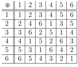
6.1 The base operation table forn=6. . . 69
6.2 The associatedZ6-coloring is strongly represented by 103=6⋅17+1. . 70
6.3 The associatedZ6-coloring is strongly represented by 7=6⋅1+1. . . 70
6.4 The associatedZ6-coloring is strongly represented by 487=6⋅81+1. . 71
6.5 The associatedZ6-coloring is strongly represented by 547=6⋅91+1. . 71
6.6 The associatedZ6-coloring is strongly represented by 13=6⋅2+1. . . . 72
6.7 Base operation table for n=7. . . 72
6.8 The associatedZ7-coloring is strongly represented by 2087=7⋅298+1. 73 6.9 The associatedZ7-coloring is strongly represented by 1429=7⋅204+1. 73 6.10 The associated Z7-coloring is strongly represented by 659=7⋅94+1. . 74
6.11 The associatedZ7-coloring is strongly represented by 21911=7⋅3130+1. 74 6.12 The associated Z7-coloring is strongly represented by 3557=7⋅508+1. 75 6.13 The associatedZ7-coloring is strongly represented by 17431=7⋅2490+1. 75 6.14 The base operation table for n=8. . . 76
6.15 Z8-coloring corresponding to the sequence(1,5,3,7). . . 77
6.16 Z8-coloring corresponding to the sequence(1,7,5,3). . . 77
6.17 Z8-coloring corresponding to the sequence(3,1,5,7). . . 77
6.24 Group corresponding to the sequence (7,5,3,1) ∶ a=1, 2, 4, or 8. . . 80
A.1 Density data for satisfactory 5-colorings . . . 112
B.1 Partial Homomorphism table for n∈ [1,16]. . . 114
B.2 Partial Homomorphism table for n∈ [17,32]. . . 115
B.3 Partial Homomorphism table for n∈ [33,39]. . . 116
B.4 Partial Homomorphism table for n∈ [40,48]. . . 116
B.5 Partial Homomorphism table for n∈ [49,54]. . . 116
C.1 A list of all groupless n for n≤500. . . 118
2.1 A χ coloring of an equilateral triangle of side length 1. . . 17
2.2 A graph that cannot be χ colored with 3 colors. . . 18
2.3 An Hexagonal Tessellation of R2, which cannot beχ colored. . . 19
2.4 A graph that cannot be χ colored with 3 colors. . . 20
2.5 G1 . . . 21
2.6 G2 . . . 22
A.1 A Matlab function witnessing a regressive function with no min-homogeneous set of size 4 . . . 106
A.2 Maple code used in the search for strong representatives . . . 107
A.3 Maple code used for data acquisition in the case of 5 colors . . . 108
A.4 Sample of the output produced by the code found in Figure A.5 when k=3. . . 110
A.5 Sage code used in the density analysis of k-representatives . . . 111
Q
R ... The set of real numbers. Zn ... The integers modulo n.
Z∗
n ... The group of units modulo n.
(a, b)... The greatest common divisor of a and b.
indg(a) ... The index ofa with respect to the primitive root g.
π(n) ... The number of primes less than or equal to n.
K =Kn ... The n-th core.
CKn ... The set of satisfactory colorings ofKn. MKn ... The set of multiplicative colorings of Kn. g⊕α ... g⊕ ⋯ ⊕g
´¹¹¹¹¹¹¹¹¹¹¹¹¹¹¹¹¹¸¹¹¹¹¹¹¹¹¹¹¹¹¹¹¹¹¹
α times
, where g is an element of an abelian group.
n ... {1,2, . . . , n}
INTRODUCTION
1.1
History of Coloring
Graph Coloring is the assignment of labels or “colors” to the edges or vertices of a graph [6]. Problems in this area (more specifically those seeking to ascertain the properties of a given coloring, or to determine whether colorings with specific properties exist) have given impetus to whole fields in combinatorics (Ramsey theory, see [10]) and set theory (partition calculus); the results often have application in number theory and analysis, among others.
Consider the following question, originally posed by Francis Guthrie in 1852, see [4].
Is it possible to color any planar map using four colors in such a way that regions sharing a common boundary, excluding boundaries which are comprised of a single point, do not share the same color?
The affirmative answer and its proof were finally attained by Kenneth Appel and Wolfgang Haken some 124 years later with the aid of computers.1 It was during this
time that the still very active area of mathematics known as Graph Coloring came to be.
1Here it is noteworthy to mention that this was the first significant mathematical result in which
theory, the chromatic number of the plane, and some of the results that have been obtained.
In Chapter 3, we extend a recent result of Andr´es Caicedo in [9] concerning regressive functions on pairs.
The remainder of the thesis deals with the main point of this thesis. The question at hand is introduced in Chapter 4, and in full generality remains unsolved. It asks for the existence of certain colorings of positive integers, generalizing a question from K¨oMaL [3]. We call such colorings satisfactory. The key notion of the n-core is introduced in Section 4.2 and discussed in detail in Section 4.3.
In Section 5.1, we give a sufficient condition, using elementary number theory, which guarantees a satisfactory coloring exists usingn colors, provided certain primes of the formnk+1 exist. In Subsection 5.1.1, we give a solution to the question posed in K¨oMaL. In Section 5.2, we identify all satisfactory colorings with at most 5 colors. Multiplicative colorings are introduced in Section 5.4, and the associated notion of partial G-homomorphism, for G an abelian group, is defined in Section 5.5.
In Chapter 6, we identify all multiplicative colorings with at most 8 colors. In Chapter 7, we discuss a related problem that provides insight to the inherent difficulty of our problem.
This thesis relied heavily on the use of scientific computing software. More specifically, we used C++, Maple, Matlab, and Sage in the acquisition of data and to some extent obtain various results throughout the thesis. As such, the main code that has been used has been included in Appendix A.
1.2
Necessary Background
We begin by providing some number theoretic results that have been fundamental in constructing satisfactory colorings. All of them can be found in [1]. We also establish some basic results on the cardinality of sets.
1.2.1 Linear Congruences
Theorem 1.1. Let m, a, b be integers with m≥1. Let d= (a, m) be the gcd of a and m. The congruence
ax≡b (modm) (1.1)
has solutions if and only if
b≡0 (modd).
Proof. Let d = (a, m). Congruence (1.1) has a solution if and only if there exist
x, y∈Z such that
particular, if (a, m) = 1, then for every b the congruence (1.1) has a unique solution modulo m.
Proof. Suppose x and y are solutions to Congruence (1.1), then
a(x−y) ≡ax−ay≡b−b≡0 (modm),
thus a(x−y) is a multiple of m and so for some integer z
a(x−y) =mz.
If (a, m) =d, then(a/d, m/d) =1 and
a
d(x−y) = m
dz.
This means that m/d divides x−y and we have that
y≡x (mod m
d ).
Moreover, every integer y of this form is a solution to Congruence (1.1). An integer congruent to x modulo m/d is congruent to x+im/d modulo m for some integer
xk≡a (modm).
The order of a modulo m is the smallest integer d such thatad≡1 (modm).
Definition 1.3. Recall that the Euler totient function φ(n) counts the number of positive integers less than or equal to n that are relatively prime to n. The number a
is a primitive root modulo m if a has order φ(m).
The following theorem guarantees the existence of primitive roots for all prime moduli. The proof can be found in [1], pp. 87–88.
Theorem 1.4. For every primep, there exist φ(p−1)pairwise incongruent primitive roots modulo p.
Corollary 1.5. The group Z∗
p is cyclic and therefore isomorphic to Zp−1.
Letpbe a prime and g be a primitive root modulop.If ais an integer andpdoes not dividea, then there exists a unique integerk ∈ {0,1, . . . , p−2}such that
a≡gk (modp).
if and only if
ap−d1 ≡1 (modp).
If a is a kth power residue modulo p, then the congruence
xk≡a (modp) (1.2)
has exactly dsolutions that are pairwise incongruent modulop, and there are precisely
(p−1)/d pairwise incongruent kth power residues modulo p.
Proof. Let l = indg(a), where g is a primitive root modulo p. Congruence (1.2) is
solvable if and only if there exists an integer y such that
gy ≡x (modp)
and
gky ≡xk≡a≡gl (modp).
This is equivalent to
ky≡l (modp−1). (1.3)
Congruence (1.3) has a solution if and only if
a(p−1)/d≡g(p−1)l/d≡1 (modp)
if and only if
(p−1)l
d ≡0 (modp−1)
if and only if
indg(a) =l≡0 (modd).
If Congruence (1.3) is solvable then by Theorem 1.2, it has exactlydsolutionsy that are pairwise incongruent modulop−1, and so Congruence (1.2) has exactlydsolutions
x=gy that are pairwise incongruent modulop.
Corollary 1.7. If p=nk+1 is prime, then{ak (modp) ∶ (a, p) =1}is a group under
multiplication modulo p, and is isomorphic to Zn.
1.2.3 Principal Number Theoretic Results
We state the well–known theorem of Dirichlet concerning primes in arithmetic pro-gressions. For proof, the reader is directed to [1], pp. 347–349.
Theorem 1.8. (Dirichlet)
Leta, m∈Z+be relatively prime. Then, there exist infinitely many primes psuch that
p ⎪⎪⎪⎪⎪
⎪⎪⎪⎪⎪
⎩−1 otherwise.
By Theorem 1.6, (n
p) ≡n p−1
2 (modp). TheQuadratic Reciprocity Law of Gauß is
the following statement, see Theorems 3.13, 3.16, and 3.17 in [1]. Theorem 1.9. (Gauß)
Let p be an odd prime.
1. The Legendre symbol ( ⋅
p) is completely multiplicative, that is
(ab
p ) = ( a p)(
b p)
for all integers a and b.
2. (2
p) = (−1) p2−1
8 .
3. If q≠p is also an odd prime, then
(q
p)( p
q) = (−1) p−1
2 q−1
2 .
The following corollary will be particularly useful.
a≡b (modm)and
a (modm) =b (modm)
are equivalent. We identify Zn=Z/nZ and {0,1, . . . , n−1} without comment.
1.2.4 Cardinality
Definition 1.12. Given sets A and B:
1. ∣A∣ ≤ ∣B∣ if and only if there is a 1−1 function f ∶A→B.
2. ∣A∣ = ∣B∣ if and only if there is a bijective function f ∶A→B.
3. ∣A∣ < ∣B∣ if and only if ∣A∣ ≤ ∣B∣ and ∣A∣ ≠ ∣B∣.
If ∣A∣ = ∣B∣, we say that A and B are equipotentor have the same cardinality.
Theorem 1.13. The Schr¨oder-Bernstein theorem. If ∣A∣ ≤ ∣B∣ and ∣B∣ ≤ ∣A∣ then,
∣A∣ = ∣B∣.
The following argument is due to Knaster and Tarski, see [22] and [23].
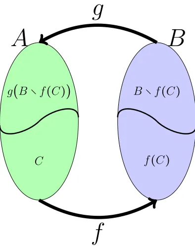
Proof. Letf ∶A→B and g ∶B →A be injections. In order to prove the theorem, we need to produce a bijection
⎪⎪⎪⎪⎪
⎩g (x), if x∉C.
If we can find such a C, we are done. If such aC exists, then, since h is a bijection, we must have that f(C) ∩g−1(A∖C) = ∅ and g−1(A∖C) ∪f(C) =B. Thus, we need
that C=A∖g(B∖f(C)).Note that, indeed, for any C satisfying this equation, the function h as defined above is a bijection, as wanted. To show there is such a C, define a function π∶ P(A) → P(A) by
π(X) =A∖g(B∖f(X)).
Now note that for any X⊆Y, we have thatπ(X) ⊆π(Y)since ifX⊆Y ⊆A, then
f(X) ⊆ f(Y) so B∖f(X) ⊇ B∖f(Y) so g(B ∖f(X)) ⊇g(B ∖f(Y)) and, finally,
A∖g(B∖f(X)) ⊆A∖g(B∖f(Y)), thusπ is monotone. Now, if we show that any monotone π∶ P(A) → P(A) has a fixed point then we are done. For such a map π, consider the collection of subsets
S= {X ⊆A∶X ⊆π(X)}.
Note that S is nonempty since it contains the empty set. Also, if X ∈ S, then
π(X) ∈ S by monotonicity. Let Y = ⋃S. Then, Y ∈S as X ⊆π(X) ⊆π(Y) for any
C f(C)
g(B∖f(C)) B∖f(C)
f
Figure 1.1: The desired mapping
then also π(Y) ∈ S, thus π(Y) ⊆ ⋃S = Y. This means that Y =π(Y), thus Y is a fixed point.
Note that up to this point, we have not invoked the axiom of choice. Had we done so, the proof of Theorem 1.13 would have been far less involved.
Definition 1.14. LetA be a set. If there is a function f ∶A→Nthat is injective, we say that A is countable. If there is such an f that is bijective, we say A is countably
infinite.
Proposition 1.15. Any subset of a countable set is countable.
Proof. Let A be a countable set, as witnessed by f. Consider B⊆A. Clearly f ↾B is
f′∶
N→A by
f′( n) =⎧⎪⎪⎪⎪⎪⎨
⎪⎪⎪⎪⎪ ⎩
f−1(n) if n∈B
a if n∉B
Then, f′ is surjective. Conversely, if f′ ∶
N →A is surjective, then A is nonempty.
Define f ∶ A → N as follows: Given a ∈ A, let f(a) be the least n ∈ N such that
f′(n) = a, which exists since f′ is surjective. Then, f is injective and, by definition, A is countable.
Proposition 1.17. A∪B is countable if and only if A and B are countable.
Proof. If A∪B is countable, by Proposition 1.15, A and B are countable since they are subsets of a countable set. Now suppose A and B are countable. If A= ∅, then
A∪B =B, and similarly if B = ∅, so we may assume that A and B are nonempty. By Lemma 1.16, there exist surjections f′ ∶
N→ A and g′ ∶
N→B. Let C =A∪B.
Defineh∶N→C by
h(2x+1) =f′(x)
and
h(2x) =g′(x),
forx∈N.Clearly,h is surjective. By Lemma 1.16, it follows that C is countable.
f ∶N×N→N
by
f(m, n) =2m3n.
By unique factorization, it is clear thatf is injective and thereforeN×Nis countable.
Remark 1.20. SinceNinjects intoN×N, it follows thatN×NandNare equipotent, by Theorem 1.13. Actually, it is possible to exhibit a bijection between the two sets without using Theorem 1.13. For example, we can take
f ∶N×N→N
to be
f(n, m) =2n(2m+1) −1,
or
(n+m+1 2 ) +m.
Proposition 1.21. A countably infinite union of countable sets is countable.
Proof. Let Ai be countable for all i∈ N. We may assume all Ai are nonempty. Let
fi∶N→Ai be surjective for alli∈N.Now define
g∶N×N→ ∞
⋃
is surjective. Let g′ ∶
N → N×N be the inverse of an f as in Remark 1.20. Then, g○g′∶
N→ ∞
⋃
i=0
Ai is surjective and the result follows.
Remark 1.22. The argument above uses the axiom of choice, by simultaneously picking a surjection fi ∶N→Ai for each i. In many specific applications of
Proposi-tion 1.21, we can exhibit these surjecProposi-tions explicitly, and therefore avoid the need to use the axiom of choice.
ForA andB sets, letAB denote the set of functions fromAtoB and let∣A∣∣B∣ be
its cardinality.
Corollary 1.23. Q is countable. Proof. Q=
∞
⋃
n=1
{m/n∣m∈Z}.
On the other hand, it is a well–known result of Cantor that Ris uncountable. We omit the argument.
Lemma 1.24. 2∣N∣= ∣ R∣.
Proof. It is well–known that the standard Cantor middle setC ⊆Rconsists of all reals of the form
x= ∞
∑
n=1
2an
3n
where each an is 0 or 1. This gives us an obvious bijection between C and the set
{0,1}N. Hence,
2∣N∣= ∣{
0,1}N∣ = ∣C∣ ≤ ∣
∣R∣ ≤2∣N∣.
The result follows from the Schr¨oder-Bernstein theorem.
Corollary 1.25. For any n∈Z+, if n>1, then n∣N∣= ∣ R∣.
Proof. It suffices to prove thatn∣N∣≤2∣N∣, by Lemma 1.24 and the Schr¨oder-Bernstein
theorem. But note that n≤2∣N∣, so n∣N∣≤ (2∣N∣)∣N∣. We claim that for any (nonempty)
sets A, B, C, we have
(∣A∣∣B∣)∣C∣= ∣ A∣∣B×C∣
.
From this, it follows that(2∣N∣)∣N∣=2∣N∣, and we are done.
To prove the claim, we exhibit a bijection π between (AB)C and AB×C. Given f ∶C→AB, defineπ(f) ∶B×C→Abyπ(f)(b, c) = (f(c))(b)for anyb∈B andc∈C.
While the Four Color Theorem is by far the most celebrated result in Graph Coloring, another result, if attained, would be heralded as equally important. The result in question is the determination of the chromatic number of the plane, as yet unknown.
Definition 2.1. The chromatic number of the plane, denoted by χ, is the smallest number of colors sufficient for coloring the plane in such a way that no two points of
the same color are unit distance apart.
Question 2.2. What is the value of χ?
Perhaps, it is the fact that this problem can be formulated in such an easy to understand fashion that makes it so intriguing. However, the simplicity of this question is merely the facade of an historically difficult problem. In fact, the best known results say thatχ is either 4, 5, 6, or 7. If a coloring of the plane is such that no two points at distance 1 have the same color, we say it is a χ coloring. If a graph cannot be colored such that no two points at distance 1 have the same color, we say the graph cannot beχ colored.
Lemma 2.3. The Chromatic number of the plane is at least 3.
Figure 2.1: Aχ coloring of an equilateral triangle of side length 1.
Proof. Consider a χ coloring of the plane, and an equilateral triangle of side length 1. Call the vertices of this triangle A, B, and C. Since A and B are a unit apart, they must be colored differently. Since C is a unit apart fromA and B, it cannot be the same color as A orB. Thus, we need at least 3 colors.
Proposition 2.4. χ≥4.
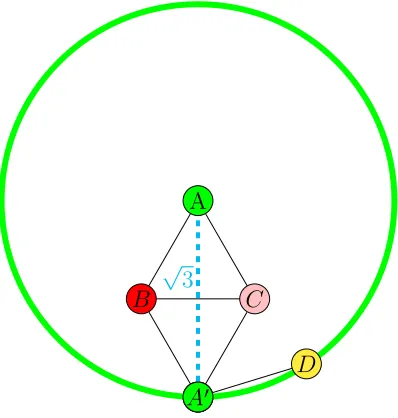
The following proof corresponds to Figure 2.2.
Proof. We proceed by contradiction. Consider aχcoloring of the plane using 3 colors, and consider an equilateral triangle of side length 1. Call its vertices A, B, and C.
Let A′ be the reflection of A across the segment BC. Note that this gives us that d(A′, B) = d(A′, C) = d(B, C) = 1 and d(A, A′) = √3. Thus, since A, B, and C all
receive different colors, it must be the case thatAandA′ have the same color. In fact,
this means that every point on the circumference of the circle of radius √3 centered atA must have the same color as A.However, for any circle with a radius at least 12, we can find 2 points on its circumference that are a unit distance apart (in fact there are infinitely many such points), which gives us the contradiction.
Proposition 2.5. χ≤7.
B √
3
C
A′ A′
D
Figure 2.2: A graph that cannot be χ colored with 3 colors.
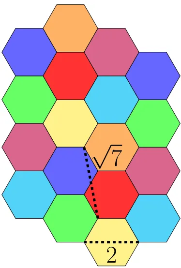
√
7
2
Figure 2.3: An Hexagonal Tessellation of R2, which cannot beχ colored.
Note that the argument of Proposition 2.4 can be easily rephrased so only 7 points need to be considered, see Figure 2.4. In some sense, this is optimal:
Proposition 2.6. Any set of at most 6 points in R2 can be χ colored with at most 3
colors.
Proof. First note that if all subsets of R2 of size at most k can be χ colored using
3 colors, then if k+1 given points cannot be χ colored with 3 colors, their resulting unit distance graph must be connected and each point must have degree at least 3.
Figure 2.4: A graph that cannot be χ colored with 3 colors.
But the only neighbors of x in the corresponding unit distance graph are vertices connected tox in this hexagon.
It follows in particular that a circle together with its center admits a χ coloring with 3 colors.
Therefore, any 4 points on R2 can be χ colored using 3 colors, since from the
above we may assume that three of the points are on the circle of radius 1 and center the fourth point.
Lemma 2.7. Any 5 points in R2 can be χ colored with 3 colors.
Proof. In a finite graph, the sum of the degrees of the vertices is twice the number of edges, so in particular it is even, and it follows that in no graph on 5 vertices can all the vertices have degree 3.
Figure 2.5: G1
Now consider the graph defined by 6 points on the plane. As above, we may assume it is connected, and each point has degree at least 3. As above, if a point has degree 5, we are done. Suppose first that there is a point x of degree 4. We claim that the sixth point is connected to at most 2 other points, which is a contradiction. In effect, the circle centered at that point meets the circle centered at x in at most 2 points, and does not contain x.
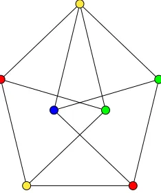
We are left with the case where the graph is 3-regular, i.e., each vertex has degree 3. But there are only 2 connected 3-regular graphs in 6 vertices, see for example [12] and references therein.
One of these graphs, call it G1, is just the complete bipartite graph K3,3. To
describe the other, call it G2, consider the vertices of a hexagon. Join opposite
vertices and every other vertex.
Note that since G1 is bipartite, it can beχ colored with 2 colors (see Figure 2.5).
Also,G2 can beχcolored with 3 colors: Color two consecutive vertices of the hexagon
with color 1, the following two with color 2, and the remaining pair with color 3 (see Figure 2.6). This completes the proof.
Remark 2.8. As a matter of fact, G1 cannot be realized as the distance-1 graph of
Figure 2.6: G2
There is a unique circle (possibly a line) that contains them, but then the 3 points on the other side of the partition cannot all be centers of unit circles containingA, B, C. On the other hand, G2 can be realized: Start with the 3 vertices of an equilateral
triangle, and translate them by one unit in some appropriate direction.
It is worth pointing out that the observation immediately preceding Proposi-tion 2.6 that the chromatic number of the plane being larger than 3 can be verified by considering an appropriate finite graph (in this case, of size 7) is not an isolated incident. This is the content of the following:
Theorem 2.9. (De Bruijn-Erd˝os)
Given any graph Gand any positive integer k, the chromatic number of Gis at most
k iff the chromatic number of any finite subgraph of G is at most k.
For a proof, see for example Theorem 3.6 in [11].
It follows in particular that there is a finite set of points in the plane whose unit distance graph has the same chromatic number as the plane. However, there are two drawbacks with the theorem.
it uses in an essential way the axiom of choice, in the form of the compactness of an appropriate product of (Hausdorff) compact spaces. Given our current knowledge, it is not unconceivable that there are models of set theory where the axiom of choice fails, every finite subset of the plane has chromatic number at most 4, and the plane itself a has larger chromatic number. These matters are discussed in detail in [4].
This short chapter builds on Caicedo [9]. It concerns the following coloring problem: For m ≤l positive integers, consider the complete graph G =G(m, l) on the set of verticesV = {m, m+1, . . . , l}. Aregressive coloring of Gis a function that assigns to each edge {a, b} of G a color c, that is a natural number strictly less than both
a and b: 0≤c<min{a, b}. These colorings are natural to consider in the context of canonical Ramsey theory.
Given a coloring f of G, a min-homogeneous set is a subset H of V such that whenever a < b <c are in H, then f({a, b}) =f({a, c}), i.e., whenever d is an edge with vertices in H, f(d) only depends on the minimum of d. We say that H is homogeneous if f is constant on edges from H.
Typically, in Ramsey theory, one proves that a coloring of a large graph admits appropriately sized homogeneous sets. This is not possible in general in this context: Simply consider the coloring f(d) =min(d) −1.
On the other hand, as shown in Section 3 of [9], for anym andnthere is an lsuch that any regressive coloring of G(m, l) admits a min-homogeneous set of at least n
elements.
3. g(4,4) ≤85.
We now give the following result.
Theorem 3.1. g(4,4) =85.
Proof. This follows by constructing a regressive coloringf ofG(4,84)which contains no min-homogeneous set of size 4. The function was constructed and verified using Matlab, modifying a coloring from [9] that proves the weaker boundg(4) ≥2g(3)+3= 77. Its definition, and the code that verifies it works, can be found in Appendix A.1.
Let us remark that the arguments of [9] give in general that
g(4, n) ≤2nn+12⋅2n−3+1
for n≥3. We close the chapter by stating without proof an improvement:
Fact 3.2. (Caicedo)
4.1
The Problem
Question 4.1. Is it possible to color the positive integers using n colors, in such a way that for any a, the numbers a,2a,3a, ..., nareceive different colors?
We call satisfactory a coloring witnessing a positive answer to Question 4.1. Question 4.1 was posted by Palvolgyi D¨om¨ot¨or to MathOverflow.net [2], a website whose stated primary goal is for users to ask and answer research level mathematics questions. The question, as D¨om¨ot¨or states in his post, is an extension of a problem originally published in the Hungarian journal K¨oMaL (K¨oz´episkolai Matematikai ´es Fizikai Lapok), a Mathematics and Physics journal primarily aimed at High School Students. In the April, 2010 issue, problem A.506 asked to show that there is a satisfactory coloring whenever n+1 is prime [3]. In full generality, Question 4.1 remains open.
In addition to asking the question of whether there are satisfactory colorings for a givenn, it is natural to ask the following:
4.2
An Example
Here we discuss how one can approach building a satisfactory coloring for 5 colors “by hand.”
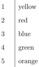
The idea is to create a table in which every column contains each color and contains no repetition. The first column, whose entries are to the left and right of the first vertical line, contains the numbers being colored on the left, and the color each receives on the right. A column is referred to ascompleteif the column uses all available colors. So, for any satisfactory coloring, every column will be complete. For instance, the following complete column represents the first column of the table used for 5 colors, and theith column is the column whose left entries are the numbersi,2i, . . . ,5i. The table is read as: Number 1 is being colored yellow, 2 is being colored red, 3 is being colored blue, 4 is being colored green and 5 is being colored orange.
1 yellow
2 red
3 blue
4 green
5 orange
way as identical.
Suppose that c is a satisfactory coloring using 5 colors,
c∶Z+→ {
1,2,3,4,5}.
We may assume that c(i) = i for i ∈ {1,2,3,4,5}. So we begin with the following table:
1 1 2 3 4 5 6 7 8 9 10
2 2 4 6 8 10 12 14 16 18 20
3 3 6 9 12 15 18 21 24 27 30
4 4 8 12 16 20 24 28 32 36 40
5 5 10 15 20 25 30 35 40 45 50
Now, we can fill in the values that are determined by the assignment of column 1. This gives us:
1 1 2 2 3 3 4 4 5 5 6 7 8 9 10
2 2 4 4 6 8 10 12 14 16 18 20
3 3 6 9 12 15 18 21 24 27 30
4 4 8 12 16 20 24 28 32 36 40
5 5 10 15 20 25 30 35 40 45 50
1 1 2 2 3 3 4 4 5 5 6 1 7 8 9 10
2 2 4 4 6 1 8 10 12 14 16 18 20
3 3 6 1 9 12 15 18 21 24 27 30
4 4 8 12 16 20 24 28 32 36 40
5 5 10 15 20 25 30 35 40 45 50
Now, consider c(10). Since 10 is in both column 2 and 5, c(10) ≠1,2,4,5 and thus
c(10) = 3. Thus, since column 2 now contains the colors 1,2,3, and 4, we see that
c(8) =5. Now our table is:
1 1 2 2 3 3 4 4 5 5 6 1 7 8 5 9 10 3
2 2 4 4 6 1 8 5 10 3 12 14 16 18 20
3 3 6 1 9 12 15 18 21 24 27 30
4 4 8 5 12 16 20 24 28 32 36 40
5 5 10 3 15 20 25 30 35 40 45 50
The following table is obtained by the same reasoning:
1 1 2 2 3 3 4 4 5 5 6 1 7 8 5 9 5 10 3
2 2 4 4 6 1 8 5 10 3 12 2 14 16 3 18 3 20 1
3 3 6 1 9 5 12 2 15 4 18 3 21 24 4 27 4 30 5
4 4 8 5 12 2 16 3 20 1 24 4 28 32 1 36 1 40 2
5 5 10 3 15 4 20 1 25 2 30 5 35 40 2 45 2 50 4
At this point, notice that no colors have been assigned yet to column 7. This is because column 7 is not dependent upon our choice of the first column. This follows from the fact that 7 is relatively prime with all numbers less than or equal to 5 or, equivalently, with 2⋅3⋅5 = 30. As a matter of fact, for every column x for which (x,30) =1, we have that c(x), c(2x), c(3x), c(4x), and c(5x) are not determined by
the first of which deals with extending a coloring of the core to all positive integers and the second, a corollary of the first, identifies the number of satisfactory colorings there are in the case of n colors, provided a coloring of the core does in fact exist.
4.3
The Core
Definition 4.3. The n-core, or simply thecore if n is understood, is the set K =Kn
of all positive integers whose prime decomposition only involves primes less than or
equal to n.
Definition 4.4. Say that X ⊆Z+ is n-appropriate iff X is nonempty and contains ai and a/j whenever a∈X, i, j≤n, and j divides a.
If X is n-appropriate, say that c∶X → {1, . . . , n} is satisfactory iff c(ai) ≠c(aj) whenevera∈X andi<j ≤n. Note that this notion coincides with the previous notion of satisfactory when X =Z+.
We denote by An the set of numbers relatively prime to n!, i.e., those positive
integers whose prime decomposition only involves prime numbers strictly larger than
n.
If X⊆Z+ and k∈
Z+, we denote byk⋅X the dilation of X by factor k:
Lemma 4.5. A set X⊆Z+ is n-appropriate iff there is a nonempty set B ⊆A
n such
that
X= ⊍
k∈B
k⋅Kn.
Moreover, if this is the case, then we have B=An∩X.
Proof. Note that Kn is n-appropriate and therefore so is k⋅Kn for any k ∈ An. It
follows that anyX of the form⊍k∈Bk⋅Kn forB ⊆An and nonempty isn-appropriate
as well.
Towards the converse, suppose now thatX isn-appropriate. From the uniqueness of prime factorization, it follows that each m ∈ Z+ can be uniquely written in the
form m =kmbm where km ∈An and bm ∈Kn. Let B = {km ∶ m∈X}. We claim that
X= ⊍k∈Bk⋅Kn.
First, note that if x ≠ y are in An, then x⋅Kn and y⋅Kn are pairwise disjoint.
Now, if k ∈B, then there is some m∈X such that k=km. By assumption, h/j ∈X
whenever h ∈ X and j ≤ n divides h. It follows immediately that in fact h/j ∈ X
wheneverh∈X andj ∈Kndivides h. In particular,k=km=m/bm ∈X. Similarly, by
assumption hi∈X whenever h∈Xand i≤n, and it follows immediately that hi∈X
whenever h∈X and i∈Kn. Therefore, k⋅Kn⊆X. This means that
⋃
k∈B
k⋅Kn⊆X.
Note that we have shown that ifX isn-appropriate andB is as above, then in fact
B =An∩X. Since the sets k⋅Kn are pairwise disjoint as k varies over Kn, it follows
that for anyn-appropriateX there is a unique B ⊆Ansuch that X= ⋃k∈Bk⋅Kn, and
we are done.
For X n-appropriate, let
CX = {c∶X→ {1, . . . , n} ∶cis satisfactory},
and denote by C the setCZ+.
The following theorem shows that C≠ ∅ iff CX ≠ ∅ for somen-appropriate setX
iff CX ≠ ∅ for all n-appropriate sets X.
In particular, it follows that the question of whether there are any satisfactory colorings for n is really a question about whether there are satisfactory colorings of the n-core Kn. In fact, the theorem shows how the satisfactory colorings of the core
completely determine all satisfactory colorings.
Theorem 4.6. 1. Suppose X ⊆Y are n-appropriate. If CY ≠ ∅, then CX ≠ ∅. In
fact, c↾X∈CX for any c∈CY.
2. Given k ∈An, if c∈Ck⋅Kn, let c ′ ∶K
n → {1, . . . , n} be the map given by c′(b) =
c(kb). Then, c′∈C
4. Suppose that CKn ≠ ∅ and X is n-appropriate. Then, c ∈ CX iff for each k∈An∩X, there is a map ck ∈CKn such that
c= ⋃
k∈An∩X
ˆ
ck k.
5. C ≠ ∅ iff CX ≠ ∅ for any n-appropriate X iff CX ≠ ∅ for some n-appropriate
set X. Moreover ifX ⊆Y aren-appropriate, then d∈CX iff d=c↾X for some
c∈CY.
Proof. (1) This is clear.
(2) Given k∈An and c∈Ck⋅Kn, if c
′ is defined as in item 2, then c′(ib) =c(kib) ≠ c(kjb) = c′(jb) for any b ∈K
n and i <j ≤ n since c is satisfactory. But, then c′ is
satisfactory as well.
(3) Conversely, if c∈CKn, k ∈An, and ˆck is defined as in item 3, then ˆck(im) = c(i(m/k)) ≠c(j(m/k)) =ˆck(jm)for anym∈k⋅Kn andi<j ≤nsincecis satisfactory.
But, then ˆck is satisfactory as well.
(4) Suppose thatCKn ≠ ∅andX isn-appropriate. For eachk∈An∩X letc
k∈C Kn
and definec= ⋃k∈An∩X
ˆ
ck
k. As shown in Lemma 4.5,k⋅Kn∩l⋅Kn= ∅ wheneverk≠l
are in An. From this, and item 3, c is well defined and has domain ⋃k∈An∩Xk⋅Kn,
which equals X, again by Lemma 4.5. Suppose m ∈X and i<j ≤n. Then, there is a unique k ∈An∩X such that mi and mj belong to k⋅Kn, and by item 3 it follows
nonempty setAn∩X, by item 1. But thenCKn≠ ∅, by item 2. It follows from item
4 that C=CZ+ ≠ ∅. But thenCY ≠ ∅ for any n-appropriate Y, again by item 1.
Finally, if X ⊆ Y are n-appropriate and c ∈ CY, then d = c ↾ X ∈ CX, by item
1. Conversely, if d ∈ CX, let e ∈ CKn, which exists as shown above. Let c
k = e for
k ∈An∩ (Y ∖X). For k∈An∩X, let ck = (d↾ k⋅Kn)′. As in item 4, we have that
c= ⋃k∈An∩Y cˆkk ∈CY. And, by construction, d =c↾X. This completes the proof of
item 5.
The importance of this theorem is paramount. It provides us with the ability to restrict our attention from all of Z+ to a set comprised of elements with an inherent
underlying structure. As such, it has played a dominant role in many of our results. The relation between arbitrary satisfactory colorings and colorings of the core detailed in Theorem 4.6 has the following corollary:
Corollary 4.7. For n>1, with C and CKn as above, if CKn≠ ∅ then ∣C∣ = ∣R∣.
Proof. As explained in Section 4.2, if there is a coloring of the core, there are at least n!≥2 such colorings (obtained by simply permuting the colors). Note that An
is countably infinite. By item 4 of Theorem 4.6, there is a bijective correspondence between the elements of C, and the set of functions from An to CKn: ∣C∣ = ∣C
An
Kn∣ ≥ n!∣An∣= ∣
R∣, by Corollary 1.25.
On the other hand, any element of C is a function from Z+ to {1, . . . , n}, so
∣C∣ ≤ ∣{1, . . . , n}Z+∣ =n∣N∣= ∣
requirement from now on.
What Theorem 4.6 and Corollary 4.7 give us can be interpreted as follows. If there is a satisfactory coloring of Kn, then there are continuum many satisfactory
colorings of Z+ using n colors. However, this abundance of colorings is a distraction
5.1
Strong Representatives
In this section, we present a condition on n ensuring the existence of satisfactory colorings with n colors. The construction below was suggested in MathOverflow by Victor Protsak, see [2].
From now on, we denote by n the set {1,2, . . . , n}.
Theorem 5.1. Let n, k∈N. If p=nk+1 is prime, and 1k,2k,3k, . . . , nk are distinct
modulo p, then the following produces a satisfactory coloring: Let
ϕ∶ {ik (modp) ∶i∈n} →n
be the bijection given by ϕ(ik (modp)) =i. Given m∈
Z+, write it as m=apr where
(a, p) =1 and r∈N. Now define c(m) =ϕ(ak (modp)).
Proof. We begin noting that by Corollary 1.7 there are exactlynpairwise incongruent nonzero kth power residues modulo nk+1. It follows that, for any b with (b, p) =1,
bk = jk (modp) for some j ∈ n. Now let d, e ∈ n. We need to argue that c(dm) =
c(em) if and only if d=e. To see this, consider dm =adpr. Thus, c(dm) =ϕ((ad)k
This leads us to the following definition.
Definition 5.2. Strong Representations.
A satisfactory coloring c∶Kn→n admits a strong representation if and only if there
exists a prime p of the form nk+1 such that 1k, . . . , nk are pairwise distinct modulo
p and, letting
ϕ∶n→ {ak (modp) ∶a∈n}
be the map
ϕ(i) =ik (modp),
then
ϕ○c(a) =ak (modp)
for all a. In this case, we call ϕ the strong representation of c, and p the associated
prime. We also say that p is a strong representative of order n (for c).
Theorem 5.1 lends us the ability to construct a satisfactory coloring in a very simple way. However, granting the existence of such a prime has eluded us. In fact, at this time, we have only found nontrivial strong representatives of order 32 or less. Here, a prime of the formp=nk+1 isnontrivialiffk>2. We call these primes trivial when k ≤2, since the requirement of Theorem 5.1 is automatically satisfied in this case, see Subsection 5.1.1.
5.1.1 Trivial Representatives
It is clear from Theorem 5.1 that if p=n+1 is prime, then the coloring
c(m) =a (modp)
where m = apr, (a, p) = 1, is a satisfactory coloring with n colors. This solves the
question originally asked in K¨oMal [3] . From the infinitude of the primes, we have:
Corollary 5.3. There are infinitely many values ofnfor which a satisfactory coloring exists.
An easy observation also gives us:
Theorem 5.4. If p=2n+1 is prime, then the map
c(m) =a2 (modp)
where m=apr, (a, p) =1, induces a satisfactory coloring with n colors.
Proof. We must show that if 1 ≤i <j ≤n, then i2 /≡ j2 (modp), as the result then
follows from Theorem 5.1. But, i2 ≡j2 (modp) implies that p∣j−i orp∣j+i. Since
3 2 7
4 1 5
5 2 11
6 1 7
7 94 659
8 2 17
9 2 19
10 1 11
11 2 23
12 1 13
13 198364 2578733
14 2 29
15 2 31
16 1 17
17 2859480 48611161
18 1 19
19 533410 10134791
20 2 41
21 2 43
22 1 23
23 2 47
24 56610508 1358652193
25 1170546910 29263672751
26 2 53
27 6700156678 180904230307
28 1 29
29 2 59
30 1 31
31 27184496610 842719394911 32 162802814486 5209690063553
33 2 67
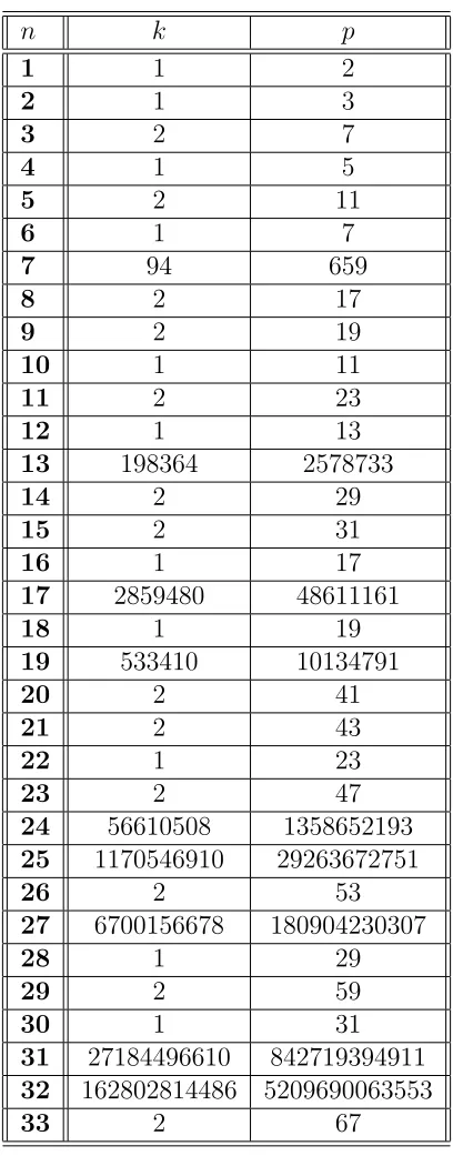
On the other hand, the primality of nk+1 for k ≥ 2 does not automatically ensure that the hypothesis of Theorem 5.1 is satisfied, as evidenced in Table 5.1. For example, if n=3, thenp=n4+1=13 is prime. However, 24=16, 34=81, and 81≡16
(mod 13).
We expect an affirmative answer to Question 4.1:
Conjecture 5.5. Satisfactory colorings exist for all n∈N.
Question 5.6. Do strong representatives of all orders exist?1
Of course, an affirmative answer to Question 5.6 implies Conjecture 5.5, but Con-jecture 5.5 may be more tractable. For example, all colorings obtained through strong representatives are multiplicative, and in fact are Zn-colorings, as defined below.
However, there are satisfactory colorings that are non-multiplicative, multiplicative colorings that are not Zn-colorings, and Zn-colorings that do not admit a strong
representation, see Sections 5.4 and 6.3.
5.2
Satisfactory Colorings with
n
≤
5
In this section, we show that if n ≤4, then there is a unique satisfactory coloring c
of Kn with n colors, subject to the convention that c(i) =i for i∈n. We also show
that there are precisely 2 satisfactory colorings of K5. This is immediate ifn=1. For
are trying to define a satisfactory coloringc.Since 6=2⋅3, we have thatc(6) ≠c(2) =2 and c(6) ≠ c(3) = 3. Thus, we are forced to define c(6) = 1. This then forces us to choose c(4) = 3 and c(9) = 2. Also, since c(12) ≠ c(4) = 3 and c(12) ≠ c(6) = 1, we have that c(12) =2.
Lemma 5.7. If c is a satisfactory coloring of K3 then, for any x∈K3, we have that
c(6x) =c(x), c(9x) =c(2x), and c(4x) =c(3x).
Proof. If x ∈ K3, then c(x), c(2x), and c(3x) are pairwise distinct. Note that
c(6x) ∉ {c(2x), c(3x)}. This it must be the case that c(6x) = c(x). Similarly,
c(4x) ∉ {c(2x), c(6x)} = {c(x), c(2x)}, soc(4x) =c(3x). Therefore,c(9x) =c(3⋅3x) = c(4⋅3x) =c(12x) =c(6⋅2x) =c(2x).
Theorem 5.8. There is a unique satisfactory coloring of K3.
Proof. By Theorem 5.1, we know that there is at least one satisfactory coloring, since 7=3⋅2+1 is prime. Let
A= {n∈K ∣ ∀c1, c2∈CK(c1(in) =c2(in) for i∈3}.
Then, 1 ∈A. Moreover, by Lemma 5.7, if n∈A, then 2n ∈A and 3n ∈A. But then
A=K.
We can easily generalize the argument above to prove the case n=4:
Lemma 5.9. If c is a satisfactory coloring of K4, then for any x∈K4, we have that
c(4⋅4x) =c(9⋅4x) =c(36x) =c(6⋅6x) =c(6x) =c(x).
Theorem 5.10. There is a unique satisfactory coloring of K4.
Proof. By Theorem 5.1, we know that there is at least one satisfactory coloring, since 5=4⋅1+1 is prime. As before, let
A= {n∈K ∣ ∀c1, c2∈CK(c1(in) =c2(in) for i∈4}.
Then, 1∈A. By Lemma 5.9, if n∈A, then {2n,3n,4n} ⊆A. But then A=K.
The situation with n = 5 is slightly more delicate. Note first that 11 =5⋅2+1, so we have a satisfactory coloring c5 given by c5(i) =i for i≤5 and c5(a) = c5(b) iff
a2 ≡b2 (mod 11) for any a, b ∈K
5. The coloring c5 satisfies c5(6) =c5(5) =5, since
36≡25 (mod 11).
Similarly, 421=5⋅84+1 is prime and
184≡1 (mod 421),
284≡279 (mod 421),
384≡252 (mod 421),
484≡377 (mod 421),
584≡354 (mod 421),
lemma follows by the same elementary reasoning as Lemmas 5.7 and 5.9 (but note the additional requirement that c(6x) =c(x)), we omit the details.
Lemma 5.11. If c is a satisfactory coloring of K5, x∈ K5, and c(6x) = c(x), then
c(20x) = c(6x) =c(x), c(25x) =c(12x) = c(2x), c(18x) =c(16x) = c(10x) = c(3x), c(24x) =c(15x) =c(4x), and c(30x) =c(9x) =c(8x) =c(5x).
Theorem 5.12. The coloring c1 defined above is the unique satisfactory coloring c
of K5 with c(6) =1.
Proof. Let
A= {n∈K∣ ∀c∈CK with c(6) =1, we have c(in) =c1(in) for i∈5 and c(6n) =c(n)}.
We have 1 ∈ A. By Lemma 5.11, if n ∈A, then also in ∈A for 2≤ i≤ 5. But then
A=K.
Theorem 5.13. The coloring c5 is the unique satisfactory coloring c of K5 with
c(6) =5. Moreover, the only satisfactory colorings of K5 are c1 and c5.
Proof. Let ϕ be the transposition (35) considered as a permutation of 5. Consider the map π that to a satisfactory coloring cof K5 assigns the coloring π(c)given by
π(c)(2a3b5d) =ϕ(c(2a5b3d)).
Note that π(c) is also satisfactory, and that π is a bijection of CK5 to itself, since in
It follows that c(10) = 1 but then π(c)(6) = ϕ(c(10)) = ϕ(1) = 1 and therefore
π(c) =c1. Since π is injective, it follows that there is a unique c with c(6) =5. But
then c=c5.
Finally, given any satisfactory coloring c of K5, since c(6) ∉ {c(2), c(3), c(4)} =
{2,3,4}, we must have thatc(6) ∈ {1,5}, which implies that c=c1 or c=c5.
5.2.1 Density of Strong Representatives
In Section 5.2, we identified the colorings c5 and c1 (with associated primes 11 and
421, respectively) as being the only satisfactory colorings for n=5. Note that there are 76 primes in the interval [12,420] and none of them are strong representatives of order 5. Now, it is only natural to ask whether 11 and 421 are the only strong representatives of order 5. This is not the case:
Example 5.14. The prime p=701=5⋅140+1 is a strong representative of order 5. In effect,
1140≡1 (mod 701),
2140≡210 (mod 701),
3140≡464 (mod 701),
4140≡638 (mod 701),
Question 5.15. Asymptotically, how many primes are strong representatives of order 5, and are the resulting colorings equidistributed among c5 and c1?
Recall that, given a realx,π(x)denotes the number of primesp≤x. Several proofs of Dirichlet’s theorem (Theorem 1.8) actually establish a version of the prime number theorem for arithmetic progressions, namely, that for any m ≥ 3, the primes are uniformly distributed among theφ(m)many congruence classes of integers relatively prime to m: For (a, m) =1, denote by π(x, m, a) the number of primes of the form
mk+a that are less than or equal to x. Then,
π(x, m, a) ∼ 1 φ(m) ⋅
x
logx
as x → ∞, where the notation means that the limit of the quotient of the two expressions is 1. Note that the right–hand side is independent of a. Put another way, about 1/φ(m) of all primes are of the form mk+a. See [1] for references.
Since 1/φ(5) =1/4 is a constant, it really makes no difference whether Question 5.15 is interpreted as asking for the proportion of strong representatives of order 5 among all primes, or among primes of the form 5k+1.
Given a realx, denote byC1(x)andC5(x), the sets of primesp≤xthat are strong
representatives of order 5 for c1 and c5, respectively, and let C(x) =C1(x) ∪C2(x).
Conjecture 5.16. 1. ∣C1(x)∣ ∼ ∣C5(x)∣ as x→ ∞.
2. lim
x→∞
is hard to imagine a scenario that would show the existence of strong representatives of a given order n without proving that there are infinitely many. For n=2, we can prove that this is the case:
Theorem 5.17. A prime p is a strong representative of order 2 iff p≡ ±3 (mod 8). In particular, there are infinitely many strong representatives of order 2.
Proof. This is immediate from Theorem 1.10: If p=2k+1 is prime, then
2k≡1 (modp)
iffp≡ ±1 (mod 8). It follows that ifp≡ ±3 (mod 8), then 1 and 2k are not congruent
modulo p.
Treating other cases seems to require a good understanding of higher order reci-procity laws. An argument that would apply to all n seems even more delicate.2
5.3
k
-representatives
Definition 5.18. Let k ∈Z+. A prime p of the form nk+1 is a k-representative if and only if p is a strong representative of order n.
It is important to note that, in general, the roles ofkandncannot be interchanged. That is, typically, if p = nk+1 is a strong representative of order n, then it is not
manyn such that p=nk+1 is a k-representative. In fact, we will show that for some values of k there are no such n.
We begin by discussing the case k=3.
Theorem 5.19. Suppose p=n3+1is prime. Then, there is an i∈n, i>2 such that i3≡1 (modp) or i3≡8 (modp). In particular, p is not a 3-representative.
Proof. Note first that−3 is a quadratic residue modulop. This follows from Theorem 1.9:
(−p3) = (−p1)(3p) = (−1)p−21(−1) p−1
2
3−1
2 (p
3) = (
n3+1 3 ) = (
1 3) =1.
Work in Zp. Note that x3 =1 and x ≠ 1 iff x2 +x+1 =0 iff 4x2+4x+4 =0 iff
(2x+1)2= −3. Also,x3 =8 and x≠2 iffx2+2x+4=0, or (x+1)2= −3.
We claim that for at least one x ∈n this must happen. This is because y2 = −3
has two solutions, one in the first half of the interval [1, p−1]. If y is actually in the first third, we are done, we get x=y−1∈n. Suppose otherwise. Note that either y
or p−y is odd. Call it z, and note that z ≤2p/3. But then x= (z−1)/2 is at most (p−1)/3, so it is in n.
The case whenk is a multiple of 4 can also be treated by elementary means. The key is the following theorem of Fermat, see Theorem 13.3 in [1]:
Theorem 5.20. (Fermat)An odd prime pis a sum of two squares iff p≡1 (mod 4). Theorem 5.21. Ifk is a multiple of4andp=nk+1isk-representative, thenp<2k2,
It follows that if p≥ 2k2, then both x and y are in n, but x2 ≡ −y2 (modp), so
xk≡yk (modp).
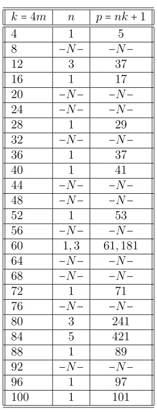
The bound onp found in Theorem 5.21 allows us for any given value ofk=4mto identify all the possible values ofp by a quick exhaustive search. Table 5.2 shows for
k =4m≤100 the values of n for which p=nk+1=n4m+1 is a k-representative. If there are no such primes, we write−N−.
We now proceed to the general case. Letting
B(t, x) = te
tx
et−1=
∞
∑
m=0
Bm(x)
tm
m!,
then
B(t, x+1) = te
txet
et−1 =
tetx(et+1−1)
et−1 =te
xt+B(t, x).
Thus
∞
∑
m=0
(Bm(x+1) −Bm(x))
tm
m! =te
xt=
∞
∑
m=0
mxm−1tm
m! ,
or
Bm(x+1) −Bm(x) =mxm−1.
It follows easily that each Bm(x) is a polynomial in x of degree m with rational
k=4m n p=nk+1
4 1 5
8 −N− −N−
12 3 37
16 1 17
20 −N− −N−
24 −N− −N−
28 1 29
32 −N− −N−
36 1 37
40 1 41
44 −N− −N−
48 −N− −N−
52 1 53
56 −N− −N−
60 1,3 61,181
64 −N− −N−
68 −N− −N−
72 1 71
76 −N− −N−
80 3 241
84 5 421
88 1 89
92 −N− −N−
96 1 97
100 1 101
A good reference on Bernoulli polynomials is [16]. Writing
Bm(x) = m
∑
k=0
( m
m−k)bkx
m−k ,
the numbersbk=Bk(0)are usually called theBernoulli numbers; they satisfyb2k+1=0
for all k≥1. In particular,
n
∑
i=1
i2m= B2m+1(n+1)
2m+1 , for m≥1.
It will be important for us to know all the rational linear factors of the polynomial
Bm(x) −Bm(0); when n is odd this reduces to determining the rational linear factors
of Bm(x). A theorem of Inkeri, see Theorem 3 in [17], solves this problem.
Theorem 5.22. (Inkeri) [17]
The rational roots of a Bernoulli polynomialBm(x)can be only0,12, and1. Moreover,
all these are roots when m>1 is odd.
With this result we are ready to prove the main result of this section.
Theorem 5.23. If k>2, then only finitely many primes are k-representatives.
1k+2k+. . .+nk≡0 (modp).
To see this, letS =1k+. . .+(p−1)k (modp). Note that the map i↦2i (modp)is a
permutation of p−1. Therefore, S ≡2kS (modp), so S ≡0 (modp). By Theorem
1.6, any nonzero kth power is congruent to ik modulo p for some i∈n, and for each
such i there are precisely k integers in p−1 realizing this congruence. But then
S≡k(1k+. . .+nk) (modp), and the claim follows.
Similarly,
n
∑
i=1
i2k≡0 (modp).
To see this, notice that, again by Theorem 1.6, there are precisely p−1
d = n
(2,n)
incon-gruent 2kth power residues modulo p, where d = (2k, p−1) = (2, n)k. If n is odd, this is precisely n, which means that the numbers 12k, . . . , n2k are all distinct and are
precisely all the nonzero 2kth powers. Ifnis even, this means that each nonzero 2kth power appears exactly twice among these numbers. In either case, it follows that the sum is zero by the same argument as in the previous paragraph.
Since
n
∑
i=0
i2k= B2k+1(n+1)
2k+1 ,
it must be the case that (nk+1)∣B2k+1(n+1). By Inkeri’s Theorem 5.22, since k>2,
the polynomial kx+1 is relatively prime to the polynomial B2k+1(x+1). But then
that there are polynomials u =Lu, B2k+1 =L1B2k+1, v =L2v∈Z[x]such that
(kx+1) ⋅u′(x) +B′
2k+1(x+1) ⋅v
′(x) =L.
Since B2k+1(n+1) ≡0 (modnk+1), evaluating the last displayed equation at x=n
gives us that p=nk+1∣L. But there are only finitely many such p.
Note that this argument does not supersede Theorems 5.19 or 5.21. For Theorem 5.21 in particular, note that the bound obtained there is in general much smaller than the bound L found in the proof of Theorem 5.23, which depends on the size of the denominator ofB2k+1(x+1).Let us illustrate this result with some examples.
Example 5.24.
n
∑
i=1 i3 =n
2(n+1)2
4 .
Clearly, ifn3+1 is prime, it does not dividen2(n+1)2. Thus, it follows that no prime
is a 3-representative.
Example 5.25.
n
∑
i=1
i4 =n(n+1)(2n+1)(3n
2+3n−1)
30 .
If n4+1 is a 4-representative, then it must divide (3n2+3n−1).But
∑
i=1
i =
12 .
If n5+1 is a 5-representative, then it must divide (2n2+2n−1).But
25(2n2+2n−1) = (10n+8)(n5+1) −33,
so n5+1 must divide 33, so n=2. Since
25=32≡ −1≢1 (mod 11),
it follows that p=11 is indeed the only 5-representative.
Example 5.27.
n
∑
i=1
i6 = n(n+1)(2n+1)(3n
4+6n3−3n+1)
42 .
If n6+1 is a 6-representative, then it must divide (3n4+6n3−3n+1). But
432(3n4+6n3−3n+1) = (216n3+396n2−66n−205)(n6+1) +637,
so n6+1 must divide 637=72⋅13, so n=1 or n=2. Since
26=64≡ −1≢1 (mod 13),
2401(3n4+6n3−n2−4n+2) = (1029n3+1911n2−616n−1284)(n7+1) +6086,
so n7+1 must divide 6086=2⋅17⋅179. However, since none of these are congruent to 1 modulo 7, it follows that there are no 7-representatives.
Example 5.29.
n
∑
i=1
i8 =n(n+1)(2n+1)(5n
6+15n5+5n4−15n3−n2+9n−3)
90 .
Ifn8+1 is a 8-representative, then it must divide(5n6+15n5+5n4−15n3−n2+9n−3).
But
262144(5n6+15n5+5n4−15n3−n2+9n−3) =
(163840n5+471040n4+104960n3−504640n2+30312n291123)(n8+1) −1077555,
so n8+1 must divide
1077555=3⋅5⋅71837.
However, since none of these are congruent to 1 modulo 8, it follows that there are no 8-representatives.
Ifn9+1 is a 9-representative, then it must divide(n2+n−1)or(2n4+4n3−n2−3n+3).
But
81(n2=n−1) = (9n+8)(n9+1) −89,
so n9+1 must divide 89≢1 (mod 9). Now, since
6561(2n4+4n3−n2−3n+3) = (1458n3+2754n2−1035n−2072)(n9+1) +21755,
n9+1 must divide 21755=5⋅19⋅229. So the only possibility is n=2. Since
29 =512≡ −1≢1 (mod 19),
it follows that p=19 is indeed the only 9-representative.
Example 5.31.
n
∑
i=1
i10= n(n+1)(2n+1)(n
2+n−1)(3n6+9n5+2n4−11n3+3n2+10n−5)
66 .
If n10+1 is a 10-representative, then it must divide
(n2+n−1),
or
106(3n6+9n5+2n4−11n3+3n2+10n−5) =
(3⋅105n5+87⋅104+113000n3−111300n2+411130n+958887)(n10+1) −5958887,
son10+1 must divide 109, or 5958887=115⋅37,son=1. It follows that p=11 is the
only 10-representative.
5.3.1 kn-densities
Definition 5.32. Letp=nk+1be a prime that is nota strong representative of order n. The kn-density, denoted kn, is given by
kn= ∣{ii∶i≠j, ik≢jk (modp), i, j∈n}∣/n.
We conclude this section with some remarks on kn-densities. As illustrated in
Appendix A.4, the numbers 3n stay rather close to 2/3 while the numbers 5n are very
close to 84/125. In [15], Noam D. Elkies discusses thekn-densities and confirms these
observations. We include his argument verbatim:
[The proof of Theorem 5.23] yields the existence of one coincidence ak ≡
bk with 0 < a < b < p/k; but in fact the number of coincidences is
asymptotically proportional to p: the count is Ck p+Ok(p1−(k)), where
Ck = (k−1)/(2k2) or (k−2)/(2k2) according as k is odd or even, and
asymptotic to((k−1)k+1)/kk; fork=5 that’s 41/125, so the proportion
with such akth root is 84/125, which matches A.Caicedo’s observed 0.672 exactly. It also gives 1− 8+1
27 = 2/3 for k = 3, matching the proportion
of cubes reported by Greg Martin in comments below; as k → ∞ the proportion of k-th powers with smallk-th roots approaches 1− (1/e).
Here’s how to estimate the number of pairs. Begin with the observation that ak =bk iff b ≡ma (modp) where m is one of the k−1 solutions of
mk ≡1 (modp) other than m =1. If k is even, we exclude also m= −1,
which is impossible with 0 <a, b <p/k. Then b ≡ma (modp) defines a lattice of index p in Z2 all of whose nonzero vectors have length ≫p(k),
because for such a vector p divides the nonzero number ak−bk, which
factors into homogeneous polynomials ina, beach of degree at mostφ(k). [This is where we usem≠ −1: ifa= −bthenak−bk=0.] Thus the solutions
of b ≡ ma (modp) with a, b ∈ (0, p/k) are the lattice points in a square of area (p/k)2, and their number is estimated by p−1(p/k)2 =p/k2, with
an error bound proportional to (perimeter)/(length of shortest nonzero vector), i.e. proportional to p1−(k). The total of C
k p+Ok(p1−(k)) then
follows by summing over allk−1 ork−2 solutions ofmk=1 (modp)other
than m= ±1, and dividing by 2 because we’ve counted each coincidence twice, as (a, b)and (b, a).
power is asymptotic to (j)p/k , while there are no such subsets with
j =k because the sum of all k solutions of ak ≡c (modp) vanishes. An
exercise in generatingfunctionological inclusion-exclusion then produces the formula ((k−1)k+1)/kk for the asymptotic proportion ofkth powers
that have no kth roots at all in (0, p/k).
The same technique also works for 0 < a < b < M with M considerably smaller thanp/k; and the resulting coincidences, when they exist, can be calculated efficiently using lattice basis reduction (which as it happens I mentioned on this forum [http://mathoverflow.net/questions/77986] a few days ago).
5.4
Multiplicative Colorings
As shown in Section 5.2, ifn≤5, then any satisfactory coloring ofKn admits a strong
representation. These colorings are very special: Fix some n, and suppose that c is a satisfactory coloring of Kn admitting a strong representation ϕ associated to the
prime p=nk+1. Let G = {ak (modp) ∣ a ∈n}. Then, as pointed out in Corollary
1.7, G≤Z∗
p is a group isomorphic toZn. Let h=ϕ○c, so
h∶Kn→G.
Since h(a) =ak (modp) for any a∈K
product in G. Note that the bijection ϕ coincides with the restriction ofh to n. Definition 5.33. A satisfactory coloring c of Kn is multiplicative iff there exists a
group (G,⋅) of order n and a bijection ϕ∶n→G such that, letting h=ϕ○c, we have that
h(ab) =h(a) ⋅h(b)
for any a, b∈Kn. In this case, we say that c is a G-coloring.
Lemma 5.34. If a satisfactory coloring ofKnis both aG1-coloring and aG2-coloring,
then G1≅G2.
Proof. If ϕ1 ∶ n → G1 and ϕ2 ∶ n → G2 witness that c is both a G1-coloring and a
G2-coloring, then ϕ1○ϕ2−1∶G2→G1 is an isomorphism.
Note that if G is as in Definition 5.33, then G is abelian, and consequently we adopt additive notation in what follows, so h is a kind of discrete logarithm. Rather than adopting this notation, we also say that h is multiplicative:
Definition 5.35. If (G,+) is an abelian group and the map h∶Kn→G satisfies that
h(ab) =h(a) +h(b) for any a, b∈Kn, we say that h is multiplicative.
Since there are only finitely many groups of any given order, there are only finitely many possibilities for G. In fact, we can easily list all the possibilities, thanks to the classification theorem for finite abelian groups, Theorem 4.3 in [1]: