Inflation interdependence in advanced economies (1 MB)

(1)

INFLATION INTERDEPENDENCE

IN ADVANCED ECONOMIES

Luis J. Álvarez, María Dolores Gadea

and Ana Gómez-Loscos

Documentos de Trabajo

N.º 1920

(2)

(3)

INFLATION INTERDEPENDENCE IN ADVANCED ECONOMIES (*)

Luis J. Álvarez (**) and Ana Gómez-Loscos (****)

BANCO DE ESPAÑA

María Dolores Gadea (***)

UNIVERSITY OF ZARAGOZA

Documentos de Trabajo. N.º 1920

2019

(*) The authors are grateful to J. Gonzalo, J. B. Gossé, D. Hendry, K. I. Inata, A. Montañés, V. Salas, A. Tagliabracci, D. Tinajero and participants in the IXt Workshop in Time Series Econometrics and the European Central Bank NIPE Workshop for their comments and suggestions. María Dolores Gadea acknowledges financial support from Spanish Ministerio de Ciencia, Innovación y Universidades (MICINN), Agencia Española de Investigación (AEI) and European Regional Development Fund (ERDF, EU) under grants C3-1-P and ECO2017-83255-C3-3-P. The views expressed in this paper are those of the authors and do not necessarily represent those of the Banco de España or the Eurosystem.

(**) Banco de España, Alcalá, 48, 28014 Madrid (Spain). Tel: +34 91 338 5042, fax: +34 338 5486 and e-mail: [email protected].

(***) Department of Applied Economics, University of Zaragoza. Gran Vía, 4, 50005 Zaragoza (Spain). Tel: +34 976 761 842, fax: +34 976 761 840 and e-mail: [email protected].

(4)

The Working Paper Series seeks to disseminate original research in economics and fi nance. All papers have been anonymously refereed. By publishing these papers, the Banco de España aims to contribute to economic analysis and, in particular, to knowledge of the Spanish economy and its international environment.

The opinions and analyses in the Working Paper Series are the responsibility of the authors and, therefore, do not necessarily coincide with those of the Banco de España or the Eurosystem.

The Banco de España disseminates its main reports and most of its publications via the Internet at the following website: http://www.bde.es.

Reproduction for educational and non-commercial purposes is permitted provided that the source is acknowledged.

(5)

Abstract

Although there is a vast literature on GDP comovement across countries, there is scant

evidence on infl ation interdependence. We analyze infl ation comovements across a wide set

of advanced economies and across the subset of euro area countries. Some of our fi ndings

are expected, such as the fact that infl ation interdependence among advanced economies

is quite relevant, but is higher among euro area countries, which show strong trade links and

a share common monetary policy, or the fact that infl ation synchronization among countries

is highest for energy prices, refl ecting common oil shocks. We also fi nd a robust puzzle:

core infl ation interdependence is fairly low and this result holds for both core goods and

services. Infl ation synchronization seems to be particularly linked to comovements in driving

variables of open economy new Keynesian Phillips curve and mark-up pricing models.

Keywords:infl ation, synchronization, fi ltering, price heterogeneity, trend infl ation.

(6)

Resumen

Aunque la literatura sobre el grado de comovimiento del PIB entre países es prolífi ca,

existe poca evidencia sobre la interdependencia de la infl ación. En este trabajo, se analizan

los comovimientos de la infl ación en un amplio conjunto de economías avanzadas,

prestando especial atención a los países del área del euro. Los resultados confi rman que

el grado de interdependencia de la infl ación entre las economías avanzadas es bastante

elevado, pero es todavía mayor entre los países de la zona del euro, que tienen fuertes vínculos comerciales y comparten una política monetaria común. Asimismo, el componente

energético muestra el mayor grado de sincronización, lo que puede refl ejar la existencia

de shocks comunes en el precio del petróleo. Un resultado inesperado, que se mantiene

robusto frente a distintas especifi caciones empíricas, es que el grado de interdependencia

de la infl ación subyacente en su conjunto es muy reducido. Este resultado se mantiene

tanto para los bienes industriales no energéticos como para los servicios. Por último,

identifi camos que la sincronización de la infl ación parece estar ligada a las variables

recogidas en los modelos neokeynesianos de curva de Phillips de economía abierta y en

los modelos de mark-up de precios.

Palabras clave: infl ación, sincronización, fi ltrado, heterogeneidad de precios, infl ación

tendencial.

(7)

1_{An alternative theoretical reason behind inﬂation comovements is that domestic inﬂation is affected by world}

output to the extent that it has an impact on real marginal costs (e.g. Gali and Monacelli (2005)). From an empirical standpoint, Borio and Filardo (2007) show that measures of global slack have explanatory power into standard Phillips curve type equations of domestic consumer price inﬂation, but this ﬁnding has not been found to be robust. See e.g. Mikolajun and Lodge (2016).

1 Introduction

Recent decades have witnessed an increase in the degree of interconnectedness among global economies associated with the growing economic and financial integration among countries. This globalization process is having an impact not only on real macroeconomic variables, but also on nominal ones, such as inflation. The aim of this paper is twofold. On the one hand, to derive a set of stylized facts on the degree of inflation comovement across countries. On the other hand, to shed some light on the macroeconomic drivers of inflation interdependence.

The open economy New Keynesian Phillips curve model provides a conceptual framework that suggests a variety of channels that potentially link inflation developments across countries. Ac-cording to this model, inflation in a given country is driven by developments in external prices, including those of commodities, business cycles and inflation expectations, so that comovements in these drivers may lead to interdependence in inflation rates of different countries. For instance, commodity prices are largely determined in global markets, so that consumer price fluctuations can be experienced in many countries at the same time. This is particularly the case for oil prices, given that their transmission to domestic retail prices is typically fairly quick. A second natural ex-planation for the comovement of national inflation rates is that real activity is also correlated across countries. That is, business cycle comovement could lead to inflation comovement, via a Phillips

Curve mechanism, as domestic inﬂation responds to changes in domestic demand.1 For instance,

the global financial crisis of 2007-2008 was followed by a prolonged period of low inflation world-wide. A third reason to explain inflation synchronization across countries rests on comovements in inflation expectations. These, in turn, may be affected by similar monetary policies and similar reactions by central banks or private agents to common shocks.

Open economy models also suggest that increases in the degree of openness, such as those brought about by globalization, may lead to higher inﬂation synchronization. In this regard, the growing importance of global value chains -i.e. cross-border trade in intermediate goods and services-, which also increase international competitive pressures on domestic price setting (Auer et al. (2017b)), would reinforce the degree of inﬂation interconnectedness.

Alternatively, mark-up pricing models suggest a highly relevant role of productivity devel-opments in inflation dynamics. Indeed, in the presence of technological spillovers, productivity growth can generate movements in inflation which are synchronized across countries (Henriksen et al. (2013)) and common sector-specific technology shocks are amplified due to input-output linkages (Auer et al. (2017a)). Finally, inflation synchronization may be explained by relative purchasing power parity theories (Taylor and Taylor (2004)).

(8)

2_{See, for instance, Kose et al. (2008) or de Haan et al. (2008).}

3_{Other contributions include Neely and Rapach (2011), Mumtaz and Surico (2012) or Forster and Tillmann (2014).}

Carriero et al. (2018) analyze the global component of inﬂation volatility.

4_{The scant evidence on heterogeneity in inﬂation synchronization is limited to CPI stripped off energy and food}

prices. See e.g. Henriksen et al. (2013).

5_{Some papers present results on inﬂation interdependence over business cycle frequencies, e.g. Henriksen et al.}

(2013).

6_{Monetarist models of trend inﬂation (e.g. McCallum and Nelson (2011)) suggest, on average a one-for-one}

relation between long-run money growth, adjusted for trend output growth, and long-run inﬂation.

contrast with that on business cycle comovement, the well-known fact that ﬂuctuations in real

economic activity tend to coincide across countries.2 Early attempts at documenting inﬂation

co-movements, such as in Wang and Wen (2007) or Henriksen et al. (2013), have relied on Pearson correlation coefﬁcients between country pairs and clearly show that headline inﬂation rates be-tween any country pairs are positively correlated. A related strand of literature, following the

seminal work by Cicarelli and Mojon (2010), estimates common/latent factor models3 and uses

variance decompositions to measure the extent to which world and country-speciﬁc components explain the variation in national inﬂation rates.

Against this background, our contribution to the literature can be summarized as follows: First, we consider to which extent inﬂation interdependence is affected by heterogeneity in price dynam-ics. i.e. are inﬂation comovements mostly due to synchronization of sectoral shocks (e.g energy) or are they broad-based? Heterogeneity in price dynamics has been documented along a number of

dimensions,4such as the degree of price stickiness ( ´Alvarez et al. (2006)), the size of price

adjust-ments (Dhyne et al. (2006)), the degree of inflation persistence (Lünnemann and Mathä (2004)), or demand elasticities, to name but a few, and it is standard in the inflation forecasting literature to consider different consumer price components (e.g. ECB (2016)) to capture heterogeneity in their response for different shocks. Moreover, optimal monetary policy is different when there is het-erogeneity in price setting (Aoki (2001) and Carvalho (2006)). Second, we systematically study to which extent the degree of inflation interdependence is different for trends, business cycle

fluctua-tions or short-term movements in inflation.5 For instance, comovement of trend inflation is likely

to be due to similarities in central banks’ inﬂation targets.6 In contrast, idiosyncratic shocks, such

as those related to changes in indirect taxes, to weather conditions, and differences in transmission mechanisms, such as those due to differences in the degree of nominal stickiness, are likely to re-sult in a low degree of inflation synchronization over the short run. Finally, inflation comovement is expected to be strongest at business cycle frequencies, reflecting the interdependence of interna-tional business cycles and its impact on nainterna-tional inflation via Phillips curve mechanisms. Third, we present evidence on inflation synchronization covering the period after the global financial crisis,

which is characterized by low inﬂation levels.7 Fourth, we focus not only on advanced economies,

but also on the subset of euro area countries, which have strong trade links and share a common monetary policy, that is a source of common demand shocks. Furthermore, euro area countries are also split into original euro area countries and newer ones. Fifth, we consider summary measures

7_{Inﬂation in advanced economies has experienced long-term swings. Inﬂation progressively rose in the 1960s and}

(9)

of inﬂation interdependence which allow us to carry out statistical inference rather than using

pair-wise country correlations that are difﬁcult to summarize.8 These summary measures can also be

used to analyze changes in inflation synchronization over time. Indeed, the degree of inflation in-terdependence is not stable over time, reflecting the time-varying importance of the different types

of shocks.9 Sixth, we analyze possible sources of inﬂation interdependence among the variables

included in open economy new Keynesian Phillips curve and mark-up pricing models.

Our main results can be summarized as follows. First, we find that inflation interdependence among advanced economies is quite relevant. Second, inflation synchronization is not broad-based and there is marked heterogeneity in the degree of interdependence across sectors. Unexpectedly, inflation comovement is fairly low for core goods and services. Third, medium run fluctuations in inflation are synchronized to a large extent, when the Phillips curve mechanism is strongest. Comovement is also substantial for trend inflation. Fourth, the degree of comovement in headline inflation has increased over our sample period, possibly reflecting the role of growing trade inte-gration and the impact of the common euro area monetary policy. Fifth, inflation synchronization among original euro area countries is higher than for all euro area countries, given that some of the newer members could not be characterized as having price stability prior to joining the euro, which in turn is higher than for advanced economies as a whole, partly due to the existence of dif-ferent central banks with difdif-ferent reaction functions. Sixth, inflation interdependence seems to be particularly linked to comovements in driving variables of open economy new Keynesian Phillips curve and mark-up pricing models. Specifically, inflation expectations, business cycles, external prices, unit labour costs and mark-ups.

After this introduction, the rest of the paper is organized as follows. Section 2 describes the data, whereas section 3 is devoted to presenting results on inﬂation interdependence along several dimensions, such as country groups, types of products or frequency bands. Section 4 presents some robustness exercises. Section 5 analyses different sources of inﬂation interdependence and section

8_{Speciﬁcally, we consider the Stock and Watson (2008) modiﬁcation of the Moran statistic used in the spatial}

correlation literature.

9_{For instance, evidence in Cicarelli and Mojon (2010) or Mumtaz and Surico (2012) suggest a lower degree of}

inﬂation synchronization early this Century than during the latest decades of the 20th Century. 6 concludes.

2 The data

(10)

newer euro area countries (NEA) to take into account that the latter only recently met the criteria needed to join this monetary union, including price convergence, and generally show a lower de-gree of trade interconnection with the rest of countries. Finally, the rest of advanced economies have country-speciﬁc monetary policies and are grouped as other advanced countries (OAC). See Table 1 for details.

To carefully assess the degree of heterogeneity in price setting, we have put together a database harmonizing, to the extent possible, country definitions. Specifically, we consider, besides the headline index, the following breakdown: (i) energy prices, which are typically quite volatile and subject to supply shocks (see Figure A1 and Table A1 in the appendix), (ii) food prices, which are also volatile and subject to sizable transitory shocks and (iii) core inflation, defined as the headline index excluding food and energy. We further decompose this core measure into (iv) non-energy industrial goods and (v) services, which are less exposed to external competition than manufactured goods.

We employ consumer price indexes for the period from January 1996 to April 2018. The series are seasonally adjusted. Data for the European countries come from Eurostat, US data from the Bureau of Labor Statistics, Canadian data from Statistics Canada and data for Japan from the Statistics Bureau of Japan.

3 Interdependence among advanced economies

A natural way to analyze inflation comovements is to consider the Pearson correlation coefficient for all country pairs. However, in our setting we would have 276 measures of synchronization for each inflation measure, which is not very practical. In order to solve this dimensionality problem, we take two different approaches. First, for each country, we simply compute the mean of its

bivariate Pearson correlation coefﬁcients with the rest of countries. Second, we use the Moran-Stock-Watson index of comovement (Stock and Watson, 2008). This measure, based on the spatial correlation literature, summarizes in a single number the degree of comovement in inﬂation across different countries. Furthermore, the distribution of this statistic is known, so that statistical infer-ence can be carried out.

3.1 A ﬁrst look at the data: Pearson correlation measures

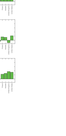
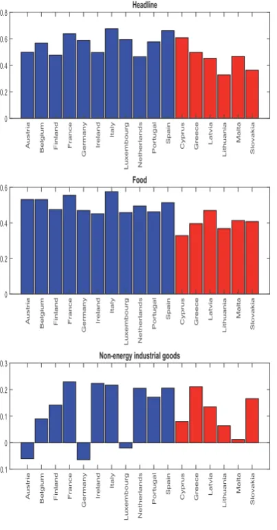
Figure 1 shows the mean correlation of a speciﬁc country with all the other countries for each of the six inﬂation measures considered. The original members of the euro are depicted in red, those of more recent incorporation in blue, whereas countries in green correspond to the rest of advanced economies.

(11)

Japanese economy stands out for its very low degree of comovement with the rest of countries. In contrast, the high mean correlation of Denmark with respect to the rest of countries could be due to the fact that the Danish krone has been linked to the euro since the beginning of our sample. We also observe a higher degree of synchronization among original euro area countries than among those euro area countries of more recent incorporation (see Figure 2).

To assess whether inflation comovements are broad-based we have also computed mean corre-lations by type of product. Our main findings are as follows: First, core inflation measures gener-ally show a low degree of comovement, a result also found in Carney (2017). This is particularly so for non-energy industrial goods, which may affected by some country-specific factors, such as the timing of sales and promotions or the use of different quality adjustment procedures. Second, comovement is very high for energy prices, reflecting the role of common oil price shocks. Fi-nally, there is a substantial degree of synchronization in food prices, probably reflecting high trade linkages.

3.2 Moran-Stock-Watson index of comovement

A more sophisticated measure of interdependence than the use of average correlations is given by the Moran-Stock-Watson (MSW) index of comovement (Stock and Watson, 2008), which summa-rizes in a single number the degree of synchronization in inﬂation developments across different

countries. Speciﬁcally, the modiﬁcation by Stock and Watson (2008) of Moran’sI_tstatistic is given

by:

MSWt= ∑

N

i=1∑ij−=11cov(πit,πjt)/N(N−1)/2

∑N_i₌1var(πit)/N (1)

where

cov(πit,πjt) = 1_k∑_st+₌_tint₋(_intk/₍2_k)_/₂₎(πis−πit)(πjs−πjt) (2)

var(πit) = 1_k∑t_s+₌_tint₋(_intk/₍2_k)_/₂₎(πis−πit)2

(3)

πit = 1_k∑t_s₌+int_t₋(_intk/₍2_k)_/₂₎πis ₍₄₎

whereπ_it is the inﬂation of country iin timet, k=61 is the rolling window, which equals to

5 years working with monthly data, andN=24, the number of countries equals 24 andint refers to

the integer part. It would be possible to build a spatial weights matrixW(w_{i j})to weigh the different

spatial units. Following Stock and Watson (2008), we have assumed that all countries behave like

neighbors and, therefore,wi j=1 if i= jand 0 ifi= j.10

(12)

This index is bounded between 1 and -1, and the higher (lower) is its absolute value the higher is the degree of comovement. Positive values mean that inﬂation rates in different countries tend to go up (down) in tandem. An advantage of this index is that its distribution is known, so that we can carry out statistical inference and compute conﬁdence intervals. Indeed, its mean and variance are given by:

E[MSWt] =−1/(N−1)

(5)

Vart[MSWt] =₍_N₋₁NS₎₍_N4₋−₂S₎₍3t_NS5₋₃₎_S2

0 (6)

where

S0=∑i∑jwi j

S1= 1₂∑i∑j(wi j+wji)2

S2=∑i(∑jwi j+∑jwji)2

S3t=

N−1_∑

ik1∑st+=intt−(intk/(2k)/2)(πis−π) 4

(N−1_∑

iπi−π)2)2

S4= (N2−3N+3)S1−NS2+S2₀

S5=S1−2NS1+6S20

and the z-score for the MSW statistic is computed as:

zt(MSWt) = MSW t−E(MSWt)

Vart(MSWt) (7)

Before exploring the time series dimension of the Moran-Stock-Watson index of comovements we have computed a scalar version by considering the whole sample. The results for advanced economies and the euro area ones are presented in Table 2. We observe that inflation comovements are important and significant for all areas. Furthermore, interdependence is higher for original euro area countries than for all euro area countries which, in turn, is higher than for advanced economies as a whole. We interpret these results as reflecting the role of high trade linkages, which are particularly high among original euro area countries, and common monetary policy in the euro area.

(13)

11_{Similarly, Carriero et al. (2018) ﬁnd that the global component of the volatility of headline inﬂation is considerably}

higher than that of core measures.

core inflation measures is significantly lower than for headline inflation ones, in line with

Car-ney (2017).11 This synchronization is particularly low for non-energy industrial goods. This low

degree of comovement, which is somewhat puzzling, is in line with simple average correlation measures and suggests that more permanent fluctuations of inflation are not heavily synchronized across countries. Our explanation is that this low degree of synchronization reflects factors such as differences across countries in sales and promotion practices, which are particularly relevant for some goods, such as clothing, footwear or electrical appliances, and which have sizable impacts

on retail prices.12 Notice also that we use ﬁnal consumer goods prices, which have a sizable

non-tradable component linked to factors, such as retailers’ labour costs such as rentals and, whose developments will generally vary across countries. We would expect export prices of these type of goods to display a higher degree of comovement. Second, the highest degree of comovement corresponds to energy prices. This is consistent with the relevance of common oil price shocks and the low degree of stickiness of these prices. Third, we ﬁnd that food prices are also quite syn-chronized, probably due to globalization of food commodity markets and the increasing existence of multinational companies. Third, regarding the geographical breakdown, the highest degree of comovement for all categories of goods and services corresponds to original euro area countries, which is higher than for the whole set of euro area countries, which, in turn is higher than for advanced economies as a whole. As mentioned above, the high degree of trade linkages and the common monetary policy in the euro area may be behind these results.

3.2.1 Interdependence over time

To analyze changes over time in the degree of inﬂation synchronization we have used two com-plementary approaches. The ﬁrst one refers to the examination of interdependence measures for two different subsamples and the second one to the use of rolling windows in the computation of measures. Notice that the subsample analysis considers a higher number of observations, so that inference is more precise than for rolling windows. This comes at the cost of subsample analysis being less accurate in the timing of changes than the one with rolling windows.

In the subsample analysis, we consider two different subsamples: the ﬁrst subsample spans the period prior to the global ﬁnancial crisis (that is, it goes from 1996 to 2007) and the second one covers the period after it (from 2008 to 2018).

Results are presented in Tables 3 and 4. Overall, inflation interdependence has increased after the global financial crisis, with the only exception of core inflation among the original euro area countries. This most likely reflects the fact that different countries increased indirect taxes and administered prices in a non-synchronized fashion after the crisis and, as a result, consumer prices

tended to show a lower degree of interdependence.13

12_{Moreover, it has also to be borne in mind that, some countries make quality adjustments in some articles, while}

others do not.

13_{Core measures, non-energy industrial goods and services, also present different patterns across subsamples and}

(14)

Some interesting information can also be obtained by analyzing developments over time of the Moran-Stock-Watson measures (see Figures 3 and 4), as some of the underlying factors, such as globalization are more relevant in the more recent period than in the past. Indeed, computing this statistic for centered rolling windows of 5 years, we find that inflation interdependence has not remained stable, but rather has tended to increase over time among advanced economies and also among euro area countries. This possibly reflects the role of growing trade integration and the role of a common euro area monetary policy in the latter group of countries.

Considering the different components for the whole sample of countries, the comovement is quite low for core inﬂation and the upward trend that was observed up to 2011 seems to be re-versing, probably reﬂecting the fact that different euro area countries passed indirect tax increases in a non-synchronized manner. In contrast, the highest degree of synchronization corresponds to energy, where a mild upward trend over time is also observed. Patterns for euro area countries as a whole are broadly similar to those of advanced economies.

As the statistical distribution of the Moran-Stock-Watson index of comovement is known, we have calculated conﬁdence intervals for advanced economies (Figure 5) and euro area ones (Figure

6) for each of the 6 types of products.14 The blue dotted lines show the conﬁdence intervals for

each of the 6 inflation measures. We find that the increase in synchronization trend is statistically significant for headline inflation and the most volatile components, energy and food. For core

inflation, comovement is significant only around the years of the global financial crisis.15

Finally, given the well documented comovement in GDP, we compare it with inflation synchro-nization. We have computed the Moran-Stock-Watson index of comovements using GDP data. We find that inflation interdependence among advanced economies is quite relevant, but it is smaller than GDP interdependence (Table 2), a result that is also found for euro area countries. Moreover, developments over time in the degree of synchronization are different for inflation and activity. For instance, whereas headline inflation interdependence has remained quite high in recent years, GDP synchronization, which peaked at the time of the global financial crisis, decreased after the

two latest European recessions (see Figures A3 and A4 in the appendix).16

3.3 Interdependence across frequency bands

The analysis above has not considered possible differences in the degree of inflation interdepen-dence regarding developments in trend inflation, business cycle fluctuations in inflation or short-term movements in inflation, despite the fact that there are theoretical reasons for expecting

dif-14_{For a comparison of developments over time of each inﬂation measure for each of the two groups of countries,}

see Figure A2 in the appendix.

15_{Considering windows of 10 years, comovement in core is signiﬁcant.}

16_{Moran-Stock-Watson indexes using quarter-on-quarter GDP growth rates have also been computed.}

Develop-ments are similar, although the degree of interdependence is lower. These results are available upon request.

(15)

syn-17_{Band-pass ﬁlters are explicit about frequency bands considered, in contrast with unobserved components models.}

Note that trend, cycle and irregular decompositions in unobserved component models implicitly consider different

frequency bands, so some care is needed when comparing across countries or type of products. See ´Alvarez and

G´omez-Loscos (2018).

18_{We have also computed mean Pearson correlation coefﬁcients and results are broadly the same.}

chronization over the short run, since they typically come into force in different countries at dif-ferent times. In turn, synchronization of trend inflation may be due to similarities in central banks’ inflation targets. Finally, inflation interdependence is expected to be strongest at business cycle fre-quencies, reflecting the synchronization of international business cycles and its impact on national inflation rates via Phillips curve mechanisms.

To decompose inﬂation into its trend, business cycle and short-term movements we use a

band-pass ﬁlter.17 Different band-pass ﬁlters can be used to carry out this decomposition. For instance,

Christiano and Fitzgerald (2003) or Baxter and King (1999) filters. In this paper, given than the Baxter and King filter involves losing observations at the start and end of the sample, we follow Henriksen et al. (2013) and use the Christiano and Fitzgerald filter. Specifically, we decompose inflation as:

πt =πtT+πBCt +πtSR (8)

where πT_t captures movements in trend inﬂation, deﬁned as cycles over 5 years, πBC_t captures

business cycle ﬂuctuations between 2 and 5 years andπ_tSR captures short-run ﬂuctuations, that is

cyclical movements below 2 years.

Decomposition of inﬂation into its trend, business cycle and short-run components are dis-played in the appendix for advanced economies (Figure A5) and euro area countries (Figure A6). To determine the source of comovements, we compute the Moran-Stock-Watson-based

synchro-nization measures separately for πT_t , πBC_t and π_tSR. Results of this interdependence measure for

advanced economies, euro area countries and original euro area countries are displayed in Table 5

for the six products and the three frequency bands considered.18

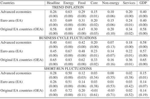
Regarding headline inflation, we find that the degree of comovement is fairly low for high frequencies, reflecting the relevance of country-specific transitory shocks. In contrast, it is highest for the medium run, when the Phillips curve mechanism is expected to be strongest. In turn, trend inflation also shows a sizable degree of comovement, although it is lower than for long-run GDP fluctuations. Interestingly, for every frequency band, the degree of interdependence is higher for original euro area countries than for all euro area countries than for all advanced economies, suggesting a relevant role of (original) euro area-specific shocks. A similar pattern applies to GDP growth.

(16)

core inﬂation, in contrast with energy prices. For all frequency bands, food prices comove more

than core ones, but less than energy ones.19

4 Robustness analysis

4.1 Leading/lagging countries

The analysis above exploits contemporaneous comovement among inflation rates, that is, the in-terrelationships of inflation across countries at the same moment of time. Here, as a robustness check, we analyze whether some countries could be leading/lagging the rest. To that end, we have computed cross-correlation coefficients of inflation in advanced economies/euro area ones with national inflation series for up to 12 leads and up to 12 lags. To save space, in Table 6 we report the highest correlation coefficient for lags 1 to 12, the contemporaneous one, and the highest cor-relation coefficient for leads 1 to 12, both for advanced economies as a whole and for euro area ones. This exercise is useful for determining whether inflation in some of the countries tends to lag or lead inflation in advanced economies or the euro area. Results show no clear evidence that any country is markedly leading or lagging advanced economies/euro area inflation developments. This allows us to discard the possibility that inflation in a particular country (for example, the United States) has been systematically leading that of the rest of the advanced economies. This supports the use of contemporaneous spatial correlation indixes.

4.2 Alternative measures of inﬂation interdependence

An alternative measure of comovement across countries is given by Pesaran’s cross dependence test (Pesaran, 2004), which measures interdependence as a function of simple correlation coefﬁcients across variables. Speciﬁcally, the measure is given by:

19_{For a comparison of developments over time of each inﬂation measure across frequency bands, see Figures A7}

and A8 in the appendix.

CD=

2T

N(N−1)(

N−1

∑

i=1

N

∑

j=i+1 ˆ

ρi j) (9)

whereT is the total number of observations,Nrefers to the number of countries andρi j to Pearson

correlation coefﬁcients. This statistic, under the null hypothesis of no cross-sectional dependence,

follows a standard Gaussian distribution forN→∞andT sufﬁciently large.

Results on Pesaran’s cross-dependance test are displayed in Table 7. We ﬁnd that results found using the Moran-Stock Watson measure are conﬁrmed by using Pesaran’s measure. That is, the lowest degree of synchronization is found for core prices and particularly so for those of

non-energy industrial goods. In contrast, non-energy prices show the highest degree of comovement.20

20_{Notice that Pesaran’s statistic depends on the number of countries considered, so, on the basis of it, no claims can}

(17)

21_{For a discussion on matrix norms, see e. g. Horn and Johnson (2012).}

22_{Note that a Frobenius norm is entry-wise, so that the similarity of matrices is done on an ”element-by-element}

basis”.

We have also applied the Peña-Rodriguez measure of cross-sectional dependence (Peña and Rodriguez, 2003). Similarly to the previous measures, we find that for all types of products and groups of countries, we reject the null hypothesis of no cross-sectional dependence.

5 Sources of inﬂation interdependence

To shed some light on the macroeconomic drivers of the degree of inflation interdependence, we consider a number of variables suggested by open economy new keynesian Phillips curve and mark-up pricing models. Then, we assess to which extent the interconnectedness of potential driving variables of inflation, in terms of their correlation matrix, mimics that of inflation

interde-pendence. To that end, we assess the distance between correlation matrices using a matrix norm.21

Speciﬁcally, to compute the degree of similarity between two correlation matrices we use the

Frobenius norm.22 This matrix norm is given by

Pπ−Pxi_F =

Tr[(Pπ−Pxi)(Pπ−Pxi)] (10)

whereP_π is the correlation matrix of inﬂation across countries, P_xi is the correlation matrix of a

potential driving variable andTris the trace operator.

The lower (higher) is the value of this norm, the closer (farther) are the two matrices. In the extreme case in which the two matrices are identical, the Frobenius distance between them is equal to zero.

As potential driving variables of inﬂation interdependence, we consider standard variables in new Keynesian Phillips curve and mark-up pricing models. An open economy new

Keyne-sian Phillis curve models explains inﬂation developments (π_t) in terms of inﬂation expectations

(Etπt+1), business cycles (yt−y∗t ) and external prices (pmt ). In stylized form:

πt =αEtπt+1+β(yt−y∗t) +γptm (11)

To proxy these variables, we use a measure of inﬂation expectations based on consumer sur-veys, business cycles are measured using GDP growth, whereas external prices are proxied using the import deﬂator.

Alternatively, mark-up pricing models explain inﬂation dynamics in terms of the growth rate

of unit labour costs (ulct) - which can be decomposed into its compensation per employee and

productivity components-, mark-ups (μt) and external prices (pm_t )

(18)

23_{GDP, employment, GDP deﬂator and import deﬂator (as a proxy for external prices) data are from Eurostat for}

the European countries, Statistics Canada for Canada, Cabinet office for Japan and Bureau of Economic Analysis for the US. Inflation expectations have been computed using the methodology of Buchmann (2009) for the European countries (see the Appendix B for details). For Japan, we apply the Carlson and Parkin (1975) methodology to Bank of Japan data. For Canada, data refer to firms and come from the Bank of Canada. For the US, they come from the St. Louis Fed FRED database. Compensation per employee data are from the OECD for all the countries, but Cyprus and Malta, for which we use Eurostat data. Unit labour costs (ULC) are computed as compensation per employee divided by productivity. The mark-up proxy is computed as the growth rate of the consumption deflator minus the growth rate of unit labour costs. Results are robust to using the GDP deflator instead of that of consumption.

In this case, we use unit labour costs data from the national accounts, whereas mark-ups are proxied by the difference between the growth rate of the GDP deﬂator and the growth rate of unit labour costs.

The statistical distribution of the Frobenius norm between two correlation matrices is unknown, so we resort to Monte Carlo techniques to estimate it. Speciﬁcally, to test for the signiﬁcance of each driver, we have designed an exercise in which we compute the empirical distribution with 10,000 replications of two random correlations matrices with a dimension equal to the number of involved countries. Figure 7 shows the kernel of the density obtained from which the p-values are calculated.

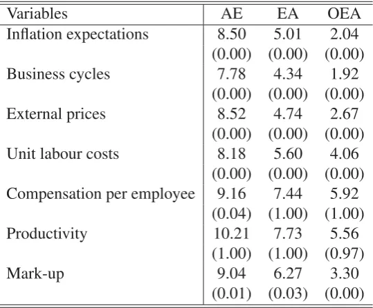
Results of the Frobenius norm, along with the p-values, are presented in Table 8.23 Our results

support both Phillips curve and mark-up pricing theories, given the similarity of interrelations of inﬂation drivers across countries (expectations, business cycles, external prices, unit labour costs and mark-ups) to interrelations of inﬂation across countries.

We also note that inﬂation interdependence between countries is similar to that of unit labor costs reﬂects similar synchronization patterns in wages (compensation per employee) develop-ments rather than those of productivity.

In order to compare the sources of inﬂation interdependence in the three geographical areas, we focus on the signiﬁcant variables (expectations, business cycles, external prices, unit labour costs and mark-ups) and we use the normalized inverse of the Frobenius norm, so that the measure does not depend on the number of countries. A higher (lower) value of this measure means that the

interdependence of the explanatory variable is more (less) close to that of inﬂation (Figure 8).24 We

show that the most related variables to inflation interdependence are, in this order, business cycles, inflation expectations and external prices. We find that the relationship between these variables and inflation interdependence is closer among the euro area, and even more, among the original euro area countries. This holds for all variables, except unit labour costs, for which the values are similar in the three areas.

6 Concluding remarks

This paper has documented that inﬂation tends to move together in advanced economies. This is particularly so for euro area countries, which have substantial trade linkages and share a common monetary policy. Moreover, there is important heterogeneity in the degree of interconnectedness

(19)

by type of product. Surprisingly, core inflation synchronization is fairly low, in clear contrast with energy prices, which are heavily dependent on oil global markets. Comovement across countries is higher when removing short-run fluctuations, which are typically quite country-specific, so that inflation interdependence is a medium to long run phenomenon. Furthermore, inflation synchro-nization has increased in recent years, against a background of globalization. However, the recent surge of protectionism points that this process may not necessarily deepen in the future.

Regarding the sources of inﬂation interdependence, we ﬁnd that comovements in driving vari-ables of open economy new Keynesian Phillips curve and mark-up pricing models help explain it.

(20)

References

[1] Adam, K. and M. Padula (2011). Inﬂation dynamics and subjective expectations in the United States. Economic Inquiry, 49(1), 13–25.

[2] Alvarez, L. J., E. Dhyne, M. Hoeberichts, C. Kwapil, H. Le Bihan, P. Lunnemann, F. Martins, R. Sabbatini, H. Stahl, P. Vermeulen and J. Vilmunen (2006). Sticky Prices in the Euro Area: A Summary of New Micro-Evidence. Journal of the European Economic Association, 4(2-3), 575–584.

[3] Alvarez, L. J. and A. Gomez-Loscos (2018). A menu on output gap estimation methods. Journal of Policy Modeling, 40(4), 827–850.

[4] Aoki, K. (2001). Optimal monetary policy responses to relative-price changes. Journal of Monetary Economics, 48(1), 55–80.

[5] Auer, R, A. A Levchenko, and P. Saure (2017a). International Inﬂation Spillovers through Input Linkages, CEPR Discussion Paper 11906, March.

[6] Auer, R., Borio, C. and A. Filardo (2017b). The globalisation of inﬂation: the growing im-portance of global value chains, CEPR Discussion Paper 11905, March.

[7] Baxter, M. and R. G. King (1999). Measuring Business Cycles. Approximate Band-Pass Filters for Economic Time Series?, The Review of Economics and Statistics, 81(4), 575– 593.

[8] Borio, C. and A. Filardo (2007). Globalisation and inﬂation: New cross-country evidence on the global determinants of domestic inﬂation, BIS Working Papers 227, Bank for Interna-tional Settlements.

[9] Buchmann, M. (2009). Nonparametric hybrid Phillips curves based on subjective expecta-tions: estimates for the Euro Area. European Central Bank. Working Paper Series 1119.

[10] Carlson, J. A., and M. Parkin (1975). Inﬂation expectations, Economica, 42(166), 123–138.

[11] Carney, M. (2017). [De]Globalisation and inﬂation. Speech given at the 2017 IMF Michel Camdessus Central Banking Lecture.

[12] Carvalho, C. (2006). Heterogeneity in price stickiness and the real effects of monetary shocks. Frontiers in Macroeconomics, 6(3).

[13] Carriero, A., Corsello, F. and M. Marcellino (2018). The global component of inﬂation volatility. Working Paper 1170, Bank of Italy.

(21)

[15] Ciccarelli, M. and B. Mojon (2010). Global inﬂation. The Review of Economics and Statis-tics, 92(3), 524–535.

[16] De Haan, J., Inklaar, R. and R. Jong-A-Pin (2008). Will business cycles in the euro area converge? A critical survey on empirical research, Journal of Economic Surveys, 22(2), 234– 273.

[17] Dhyne, E., Alvarez, L.J., H. Le Bihan, G. Veronese, D. Dias, J. Hoffman, N. Jonker, P. Lunnemann, F. Rumler and J. Vilmunen (2006). Price changes in the euro area and the United States: Some facts from individual consumer price data. Journal of Economic Perspectives, 20(2), 171–192.

[18] European Central Bank (2016). A guide to the Eurosystem/ECB staff macroeconomic pro-jection exercises, July 2016. European Central Bank.

[19] Forster, M. and P. Tillmann (2014). Reconsidering the international comovement of inﬂation. Open Economies Review, 25(5), 841–863.

[20] Henriksen, E., Kydland, F. E. and R. Sustek (2013). Globally correlated nominal ﬂuctuations. Journal of Monetary Economics, 60(6), 613–631.

[21] Horn, R.A., and C.R. Johnson (2012). Matrix analysis. Cambridge University Press.

[22] Gali, J. and T. Monacelli (2005). Monetary policy and exchange rate volatility in a sMall open economy. The Review of Economic Studies, 72(3), 707–734.

[23] Kose, M. A., Otrok, C. and C. H. Whiteman (2008). Understanding the evolution of world business cycles, Journal of International Economics, 75(1), 110–130.

[24] Lunnemann, P. and T. Y. Matha (2004). How persistent is disaggregate inﬂation? An analysis across EU 15 countries and HICP sub-indices. ECB Working Paper No. 415.

[25] McCallum, B. T. and E. Nelson (2011). Money and inﬂation: Some critical issues. In Hand-book of monetary economics, 3, pp. 97–153.

[26] Mikolajun, I. and D. Lodge (2016). Advanced economy inﬂation: the role of global factors. Working Paper No. 1948. European Central Bank.

[27] Mumtaz, H. and P. Surico (2012). Evolving international inﬂation dynamics: world and country-speciﬁc factors. Journal of the European Economic Association, 10(4), 716–734.

[28] Neely, C. J. and D. E. Rapach (2011). International comovements in inﬂation rates and coun-try characteristics. Journal of International Money and Finance, 30(7), 1471–1490.

(22)

[30] Pesaran, M. H. (2004). General Diagnostic Tests for Cross Section Dependence in Panels, Cambridge Working Papers in Economics 0435, Faculty of Economics, University of Cam-bridge.

[31] Stock, J. H. and M. Watson (2008). The evolution of national and regional factors in US housing construction. Volatility and time series econometrics: essays in honor of Robert F. Engle, eds. Bollerslev T, Russell J, Watson M. Oxford: Oxford University Press.

[32] Taylor, A. M. and M. P. Taylor (2004). The Purchasing Power Parity Debate. Journal of Economic Perspectives, 18 (4), 135–158.

(23)

Table 1: Geographical and product breakdown

Tables

Geographical breakdown Euro Area countries

Country Original EA Newer EA Other advanced

aggregates countries (OEA) countries (NEA) countries (OAC)

Advanced economies Austria Cyprus Canada

European Union (EU) Belgium Greece Denmark

Euro Area (EA) Finland Latvia Japan

France Lithuania Poland

Germany Malta Sweden

Ireland Slovakia United Kingdom

Italy United states

Luxembourg Netherlands

Portugal Spain

Product breakdown Headline inﬂation

1. Energy 2. Food

3. Core inﬂation (Headline ex food and energy) 3.1 Non-energy industrial goods

3.2 Services

Table 2: Moran-Stock-Watson measures of comovements

Countries Headline Energy Food Core Non-energy Services GDP

Advanced economies 0.30 0.60 0.32 0.15 0.09 0.19 0.42

(0.00) (0.00) (0.00) (0.01) (0.07) (0.00) (0.00)

Euro area (EA) 0.36 0.65 0.36 0.20 0.14 0.22 0.42

(0.00) (0.00) (0.00) (0.02) (0.06) (0.01) (0.01)

Original EA countries (OEA) 0.59 0.84 0.51 0.29 0.18 0.31 0.55

(0.00) (0.00) (0.00) (0.04) (0.14) (0.03) (0.00)

(24)

Table 4: Moran-Stock-Watson measures of comovements (2008M1-2018M4)

Countries HICP Energy Food Core Non-energy Services

Advanced economies 0.05 0.50 0.18 0.07 0.10 0.06

(0.24) (0.00) (0.00) (0.13) (0.06) (0.16)

Euro area (EA) 0.03 0.55 0.22 0.04 0.08 0.02

(0.39) (0.00) (0.01) (0.34) (0.20) (0.43)

Original EA countries (OEA) 0.40 0.81 0.43 0.41 0.32 0.31

(0.01) (0.00) (0.00) (0.01) (0.02) (0.03)

Note. p-values in parentheses.

Table 3: Moran-Stock-Watson measures of comovements (1996M1-2007M12)

(0.00) (0.00) (0.00) (0.00) (0.33) (0.00)

Euro area (EA) 0.55 0.74 0.51 0.23 0.12 0.25

(0.00) (0.00) (0.00) (0.01) (0.10) (0.00)

(0.00) (0.00) (0.00) (0.09) (0.25) (0.06)

(25)

Table 5: Moran-Stock-Watson measures of comovements across frequency bands

Countries Headline Energy Food Core Non-energy Services GDP

TREND INFLATION

(0.00) (0.00) (0.00) (0.01) (0.06) (0.00) (0.00)

Euro area (EA) 0.33 0.69 0.31 0.20 0.15 0.24 0.40

(0.00) (0.00) (0.00) (0.02) (0.06) (0.01) (0.00)

(0.00) (0.00) (0.00) (0.03) (0.10) (0.02) (0.00)

BUSINESS CYCLE FLUCTUATIONS

(0.00) (0.00) (0.00) (0.00) (0.13) (0.00) (0.00)

Euro area (EA) 0.45 0.67 0.48 0.23 0.14 0.22 0.57

(0.00) (0.00) (0.00) (0.01) (0.07) (0.01) (0.00)

(0.00) (0.00) (0.00) (0.02) (0.16) (0.01) (0.00)

SHORT-RUN FLUCTUATIONS

(0.00) (0.00) (0.03) (0.34) (0.55) (0.38) (0.01)

Euro area (EA) 0.26 0.51 0.14 0.03 0.01 0.03 0.14

(0.00) (0.00) (0.06) (0.38) (0.53) (0.42) (0.07)

Original EA countries (OEA) 0.45 0.72 0.20 -0.01 -0.03 0.02 0.14

(0.00) (0.00) (0.11) (0.61) (0.71) (0.52) (0.19)

(26)

Table 7: Pesaran’s cross-dependence test (CD)

Note. We report the highest correlation coefﬁcient for lags 1 to 12, the contemporaneous one, and the highest correlation coefﬁcient for leads 1 to 12.

Table 6: Cross-correlations of inﬂation of each country with Advanced economies and the Euro Area

Countries Advanced economies Euro Area

lags comtemp. leads lags comtemp. leads

Austria 0.69 0.73 0.71 0.77 0.80 0.78

Belgium 0.71 0.76 0.75 0.79 0.82 0.79

Finland 0.39 0.45 0.51 0.60 0.64 0.66

France 0.77 0.82 0.79 0.92 0.95 0.91

Germany 0.79 0.83 0.79 0.87 0.90 0.86

Ireland 0.53 0.56 0.57 0.62 0.64 0.63

Italy 0.66 0.70 0.72 0.88 0.92 0.92

Luxembourg 0.83 0.86 0.81 0.88 0.89 0.84

Netherlands 0.34 0.39 0.50 0.61 0.64 0.66

Portugal 0.63 0.65 0.65 0.79 0.79 0.77

Spain 0.79 0.80 0.78 0.91 0.92 0.89

Cyprus 0.62 0.67 0.69 0.75 0.78 0.77

Greece 0.49 0.51 0.49 0.62 0.62 0.59

Latvia 0.53 0.57 0.61 0.55 0.58 0.60

Lithuania 0.34 0.39 0.47 0.34 0.38 0.42

Malta 0.30 0.38 0.53 0.47 0.52 0.57

Slovakia 0.38 0.40 0.40 0.39 0.40 0.39

Canada 0.68 0.73 0.66 0.59 0.61 0.56

Denmark 0.62 0.67 0.66 0.78 0.80 0.78

Japan 0.15 0.20 0.22 -0.13 -0.10 -0.05

Poland 0.23 0.25 0.24 0.16 0.17 0.17

Sweden 0.31 0.36 0.35 0.48 0.49 0.47

United Kingdom 0.37 0.42 0.44 0.47 0.51 0.53

United States 0.94 0.99 0.92 0.77 0.78 0.73

(0.00) (0.00) (0.00) (0.00) (0.00) (0.00)

Euro area (EA) 98.29 133.35 86.78 44.36 21.98 56.43

(0.00) (0.00) (0.00) (0.00) (0.00) (0.00)

(27)

Table 8: Inﬂation sources (Frobenius norm)

Variables AE EA OEA

Inﬂation expectations 8.50 5.01 2.04

(0.00) (0.00) (0.00)

Business cycles 7.78 4.34 1.92

(0.00) (0.00) (0.00)

External prices 8.52 4.74 2.67

(0.00) (0.00) (0.00)

Unit labour costs 8.18 5.60 4.06

(0.00) (0.00) (0.00)

Compensation per employee 9.16 7.44 5.92

(0.04) (1.00) (1.00)

Productivity 10.21 7.73 5.56

(1.00) (1.00) (0.97)

Mark-up 9.04 6.27 3.30

(0.01) (0.03) (0.00)

(28)

Figure 1: Mean correlation coefﬁcients of each country with the rest by group

Figures

+HDGOLQH

Austria _Belgium Finland France

Germany Ireland Italy Luxembourg Netherlands Portugal Spain

Cyprus Greece Latvia

Lithuania

Malta

Slovakia Canada

Denmark

Japan Poland _Sweden

United Kingdom United States 0 0.2 0.4 0.6 0.8 1 Energy

Lithuania

Malta

Slovakia Canada

Denmark

United Kingdom United States 0 0.2 0.4 0.6 0.8 1 Food

Lithuania

Malta

Slovakia Canada

Denmark

United Kingdom United States 0 0.2 0.4 0.6 0.8

1 Core inflation

Lithuania

Malta

Slovakia Canada

Denmark

United Kingdom United States 0 0.2 0.4 0.6 0.8 1

Non-energy industrial goods

Austria _Belgium Finland France Germany Ireland Italy Luxembourg Netherlands Portugal Spain _Cyprus Greece Latvia Lithuania Malta

Slovakia Canada _Denmark Japan Poland Sweden

United Kingdom United States 0 0.2 0.4 0.6 0.8 1 Services

Austria _Belgium Finland France Germany Ireland Italy Luxembourg Netherlands Portugal Spain _Cyprus Greece Latvia Lithuania Malta

Slovakia Canada _Denmark Japan Poland Sweden

(29)

Figure 2: Mean correlation coefﬁcients of each EA country with the rest by group

+HDGOLQH

Lithuania Malta Slovakia 0 0.2 0.4 0.6 0.8 Energy

Lithuania Malta Slovakia 0 0.2 0.4 0.6 0.8 1 Food Austria

Belgium Finland France _Germany Ireland

Italy

Portugal

Spain

Lithuania Malta Slovakia 0 0.2 0.4

0.6 Core inflation

Austria

Italy

Portugal

Spain

Lithuania Malta Slovakia -0.2 0 0.2 0.4 0.6

Non-energy industrial goods

Austria

Italy

Portugal

Spain

Lithuania Malta Slovakia -0.1 0 0.1 0.2 0.3 Services Austria

Italy

Portugal

Spain

(30)

Figure 4: Moran-Stock-Watson measure of comovements. Euro area countries (window=5 years) 1997 1998 1999 2000 2001 2002 2003 2004 2005 2006 2007 2008 2009 2010 2011 2012 2013 2014 2015 2016 2017 2018

0 0.1 0.2 0.3 0.4 0.5 0.6 0.7 0.8 0.9 1

+HDGOLQH Energy Food Core inflation Non-energy industrial goods Services

Figure 3: Moran-Stock-Watson measure of comovements. Advanced countries (window=5 years)

1997 1998 1999 2000 2001 2002 2003 2004 2005 2006 2007 2008 2009 2010 2011 2012 2013 2014 2015 2016 2017 2018

0 0.1 0.2 0.3 0.4 0.5 0.6 0.7 0.8 0.9 1

(31)

1997 1998 1999 2000 2001 2002 2003 2004 2005 2006 2007 2008 2009 2010 2011 2012 2013 2014 2015 2016 2017 2018 0 0.2 0.4 0.6 0.8 1 +HDGOLQH It CI-high CI-low

1997 1998 1999 2000 2001 2002 2003 2004 2005 2006 2007 2008 2009 2010 2011 2012 2013 2014 2015 2016 2017 2018

0.4 0.5 0.6 0.7 0.8 0.9 1 Energy It CI-high CI-low

1997 1998 1999 2000 2001 2002 2003 2004 2005 2006 2007 2008 2009 2010 2011 2012 2013 2014 2015 2016 2017 2018

0 0.2 0.4 0.6 0.8 1 Food It CI-high CI-low

1997 1998 1999 2000 2001 2002 2003 2004 2005 2006 2007 2008 2009 2010 2011 2012 2013 2014 2015 2016 2017 2018

0 0.2 0.4 0.6 0.8

It CI-high CI-low

1997 1998 1999 2000 2001 2002 2003 2004 2005 2006 2007 2008 2009 2010 2011 2012 2013 2014 2015 2016 2017 2018

0 0.2 0.4 0.6 0.8

1 Non-energy industrial goods

It CI-high CI-low

1997 1998 1999 2000 2001 2002 2003 2004 2005 2006 2007 2008 2009 2010 2011 2012 2013 2014 2015 2016 2017 2018

0 0.2 0.4 0.6 0.8 1 Services It CI-high CI-low

(32)

Figure 6: Moran-Stock-Watson measure of comovements. Euro area countries (window=5 years, along with 0.95 conﬁdence intervals)

1997 1998 1999 2000 2001 2002 2003 2004 2005 2006 2007 2008 2009 2010 2011 2012 2013 2014 2015 2016 2017 2018

-0.2 0 0.2 0.4 0.6 0.8 1 +HDGOLQH It CI-high CI-low

1997 1998 1999 2000 2001 2002 2003 2004 2005 2006 2007 2008 2009 2010 2011 2012 2013 2014 2015 2016 2017 2018

0.4 0.5 0.6 0.7 0.8 0.9 1 Energy It CI-high CI-low

1997 1998 1999 2000 2001 2002 2003 2004 2005 2006 2007 2008 2009 2010 2011 2012 2013 2014 2015 2016 2017 2018

0 0.2 0.4 0.6 0.8 1 Food It CI-high CI-low

1997 1998 1999 2000 2001 2002 2003 2004 2005 2006 2007 2008 2009 2010 2011 2012 2013 2014 2015 2016 2017 2018

-0.2 0 0.2 0.4 0.6 0.8

It CI-high CI-low

1997 1998 1999 2000 2001 2002 2003 2004 2005 2006 2007 2008 2009 2010 2011 2012 2013 2014 2015 2016 2017 2018

-0.2 0 0.2 0.4 0.6 0.8

It CI-high CI-low

1997 1998 1999 2000 2001 2002 2003 2004 2005 2006 2007 2008 2009 2010 2011 2012 2013 2014 2015 2016 2017 2018

(33)

Figure 8: Sources of inﬂation interdependence

4 5 6 7 8 9 10 11

0 0.2 0.4 0.6 0.8 1 1.2 1.4 1.6 1.8

AE EA OEA

(34)

Countries Headline Energy Food Core inﬂation non-energy Services industrial goods

Mean Median St.dev. Mean Median St.dev. Mean Median St.dev. Mean Median St.dev. Mean Median St.dev. Mean Median St.dev. Advanced economies 1.87 1.83 0.96 3.12 3.77 9.64 2.12 1.96 1.16 1.74 1.76 0.36 0.13 0.09 0.53 2.41 2.45 0.54 European Union 1.76 1.85 0.89 3.10 2.81 5.81 2.28 2.04 1.44 1.42 1.47 0.39 0.36 0.38 0.36 2.21 2.25 0.58 Euro area 1.65 1.84 0.89 2.92 2.52 6.40 2.06 1.94 1.33 1.37 1.36 0.42 0.64 0.60 0.35 1.90 1.87 0.57 Austria 1.73 1.72 0.85 2.13 1.63 6.89 2.13 2.05 1.60 1.62 1.61 0.52 0.68 0.63 0.70 2.26 2.25 0.65 Belgium 1.85 1.78 1.09 3.01 2.38 9.38 2.29 2.16 1.51 1.50 1.46 0.42 0.83 0.86 0.61 2.03 2.04 0.48 Finland 1.63 1.43 1.04 2.92 2.26 6.78 1.74 1.38 2.69 1.45 1.50 0.67 0.01 0.00 0.79 2.51 2.56 0.83 France 1.45 1.51 0.87 2.66 1.83 6.61 1.96 1.65 1.60 1.14 1.04 0.50 0.19 0.14 0.50 1.77 1.65 0.72 Germany 1.39 1.41 0.80 3.01 2.74 6.06 1.88 1.86 1.46 1.06 1.14 0.41 0.57 0.66 0.56 1.41 1.38 0.49 Ireland 1.74 1.92 1.89 3.37 3.25 6.95 1.73 1.53 2.67 1.50 1.65 1.81 -1.89 -1.54 2.19 3.20 3.07 1.89 Italy 1.85 2.04 0.99 2.44 2.51 6.46 2.01 1.78 1.42 1.73 1.87 0.66 1.28 1.37 0.60 2.09 2.24 0.85 Luxembourg 2.09 2.17 1.40 2.57 2.44 10.41 3.04 2.97 1.22 1.73 1.88 0.53 1.09 1.12 0.55 2.36 2.49 0.71 Netherlands 1.83 1.70 1.18 3.54 4.17 5.66 2.05 1.82 1.95 1.56 1.29 0.98 0.56 0.41 1.22 2.32 2.17 1.10 Portugal 2.00 2.19 1.36 3.29 3.02 5.72 1.93 2.26 2.12 1.79 1.84 1.21 0.42 0.34 1.48 2.82 2.79 1.36 Spain 2.12 2.39 1.45 2.97 2.57 8.14 2.54 2.52 1.75 1.84 2.25 1.03 0.90 0.96 0.95 2.60 3.21 1.36 Cyprus 1.85 2.07 1.84 4.75 5.34 11.68 3.22 3.40 3.08 0.97 1.00 1.08 -0.43 -0.59 1.42 2.08 2.32 1.57 Greece 2.35 2.96 1.97 4.16 3.10 10.98 2.78 2.74 2.20 2.01 2.54 2.12 1.02 1.60 2.12 2.66 3.19 2.55 Latvia 3.74 2.98 3.79 5.60 5.01 7.60 4.44 2.52 5.11 3.11 1.93 3.58 1.61 1.30 2.95 4.54 3.00 4.82 Lithuania 2.83 2.31 3.17 5.40 5.73 7.87 3.06 2.58 4.39 2.20 1.61 2.97 0.43 0.08 2.55 4.45 3.45 4.03 Malta 2.24 2.29 1.24 4.16 3.02 8.36 3.24 2.90 2.00 1.81 1.70 1.11 0.72 0.76 1.01 2.64 2.36 1.79 Slovakia 3.94 3.51 3.50 7.16 4.16 11.93 3.20 3.72 2.83 3.51 2.51 2.77 1.63 0.85 2.55 5.32 4.21 3.74 Canada 1.83 1.83 0.86 3.00 4.07 8.44 2.29 1.99 1.53 1.66 1.61 0.56 2.28 2.18 0.62 0.41 0.38 1.20 Denmark 1.63 1.69 0.97 2.61 1.75 5.12 1.83 1.48 2.08 1.42 1.40 0.63 0.01 0.05 0.90 2.50 2.50 0.74 Japan 0.14 -0.10 1.07 4.14 1.89 10.70 0.37 -0.00 1.65 0.37 -0.00 1.65 -1.06 -1.23 1.69 0.32 0.16 0.89 Poland 3.71 2.76 3.82 5.43 5.53 5.55 3.77 3.41 3.63 3.38 1.78 4.22 1.98 0.35 4.03 4.84 2.69 4.70 Sweden 1.44 1.35 0.84 2.97 3.16 4.45 1.89 1.60 1.80 1.04 0.93 0.58 -0.08 -0.18 0.93 1.86 1.83 0.64 United Kingdom 1.95 1.81 1.06 4.07 3.63 6.15 2.57 2.44 2.26 1.53 1.47 0.67 -0.83 -1.05 1.64 3.26 3.33 0.62 United States 2.13 2.09 1.19 3.01 4.11 12.17 2.32 2.21 1.31 2.00 2.08 0.43 0.09 0.12 0.97 2.74 2.83 0.66

Table A1. Descriptive statistics

(35)

(36)

Note. Conﬁdence intervals at 5%.

1997 1998 1999 2000 2001 2002 2003 2004 2005 2006 2007 2008 2009 2010 2011 2012 2013 2014 2015 2016 2017 2018

-0.2 0 0.2 0.4 0.6 0.8 1

Headline (long-run)

1997 1998 1999 2000 2001 2002 2003 2004 2005 2006 2007 2008 2009 2010 2011 2012 2013 2014 2015 2016 2017 2018

0 0.2 0.4 0.6 0.8

1 Headline (medium-run)

It (AE) CI-high (AE) CI-low (AE) It (EA) CI-high (EA) CI-low (EA)

1997 1998 1999 2000 2001 2002 2003 2004 2005 2006 2007 2008 2009 2010 2011 2012 2013 2014 2015 2016 2017 2018

0 0.2 0.4 0.6 0.8

1 Headline (short-run)

1997 1998 1999 2000 2001 2002 2003 2004 2005 2006 2007 2008 2009 2010 2011 2012 2013 2014 2015 2016 2017 2018

-0.2 0 0.2 0.4 0.6 0.8

1 Core inflation (long-run)

1997 1998 1999 2000 2001 2002 2003 2004 2005 2006 2007 2008 2009 2010 2011 2012 2013 2014 2015 2016 2017 2018

-0.2 0 0.2 0.4 0.6 0.8

1 Core inflation (medium-run)

1997 1998 1999 2000 2001 2002 2003 2004 2005 2006 2007 2008 2009 2010 2011 2012 2013 2014 2015 2016 2017 2018

-0.2 0 0.2 0.4 0.6 0.8

1 Core inflation (short-run)

(37)

1997Q1 1998Q1 1999Q1 2000Q1 2001Q1 2002Q1 2003Q1 2004Q1 2005Q1 2006Q1 2007Q1 2008Q1 2009Q1 2010Q1 2011Q1 2012Q1 2013Q1 2014Q1 2015Q1 2016Q1 2017Q1 0

0.1 0.2 0.3 0.4 0.5 0.6 0.7 0.8 0.9 1

It CI-high CI-low

Figure A3. Moran-Stock-Watson measure of comovements of GDP. Advanced economies (win-dow=5 years

1997Q1 1998Q1 1999Q1 2000Q1 2001Q1 2002Q1 2003Q1 2004Q1 2005Q1 2006Q1 2007Q1 2008Q1 2009Q1 2010Q1 2011Q1 2012Q1 2013Q1 2014Q1 2015Q1 2016Q1 2017Q1 -0.1

0 0.1 0.2 0.3 0.4 0.5 0.6 0.7 0.8 0.9

It CI-high CI-low

(38)

Figure A5. Decomposition of inﬂation rates into frequency bands (Christiano and Fitzgerald ﬁlter). Advanced economies

1997 1998 1999 2000 2001 2002 2003 2004 2005 2006 2007 2008 2009 2010 2011 2012 2013 2014 2015 2016 2017 2018

-2 0 2 4

6 +HDGOLQH

1997 1998 1999 2000 2001 2002 2003 2004 2005 2006 2007 2008 2009 2010 2011 2012 2013 2014 2015 2016 2017 2018

-30 -20 -10 0 10 20

30 Energy

1997 1998 1999 2000 2001 2002 2003 2004 2005 2006 2007 2008 2009 2010 2011 2012 2013 2014 2015 2016 2017 2018

-4 -2 0 2 4

6 Food

1997 1998 1999 2000 2001 2002 2003 2004 2005 2006 2007 2008 2009 2010 2011 2012 2013 2014 2015 2016 2017 2018

-1 0 1 2

1997 1998 1999 2000 2001 2002 2003 2004 2005 2006 2007 2008 2009 2010 2011 2012 2013 2014 2015 2016 2017 2018

-2 -1 0 1

1997 1998 1999 2000 2001 2002 2003 2004 2005 2006 2007 2008 2009 2010 2011 2012 2013 2014 2015 2016 2017 2018

-1 0 1 2 3

4 Services

(39)

Figure A6. Decomposition of inﬂation rates into frequency bands (Christiano and Fitzgerald ﬁlter). Euro area

1997 1998 1999 2000 2001 2002 2003 2004 2005 2006 2007 2008 2009 2010 2011 2012 2013 2014 2015 2016 2017 2018

-2 -1 0 1 2 3

4 HHDGOLQH

1997 1998 1999 2000 2001 2002 2003 2004 2005 2006 2007 2008 2009 2010 2011 2012 2013 2014 2015 2016 2017 2018

-20 -10 0 10

20 Energy

1997 1998 1999 2000 2001 2002 2003 2004 2005 2006 2007 2008 2009 2010 2011 2012 2013 2014 2015 2016 2017 2018

-4 -2 0 2 4

6 Food

1997 1998 1999 2000 2001 2002 2003 2004 2005 2006 2007 2008 2009 2010 2011 2012 2013 2014 2015 2016 2017 2018

-0.5 0 0.5 1 1.5 2

2.5 Core inflation

1997 1998 1999 2000 2001 2002 2003 2004 2005 2006 2007 2008 2009 2010 2011 2012 2013 2014 2015 2016 2017 2018

-1 0 1 2

1997 1998 1999 2000 2001 2002 2003 2004 2005 2006 2007 2008 2009 2010 2011 2012 2013 2014 2015 2016 2017 2018

-1 0 1 2 3

4 Services

(40)

1997 1998 1999 2000 2001 2002 2003 2004 2005 2006 2007 2008 2009 2010 2011 2012 2013 2014 2015 2016 2017 2018 0 0.1 0.2 0.3 0.4 0.5 0.6 0.7 0.8 0.9 1 HHDGOLQH Energy Food Core inflation Non-energy industrial goods

Services

(a)Long-run ﬂuctuations

Services

(b)Medium-run ﬂuctuations

Services

(c)Short-run ﬂuctuations

(41)

Figure A8. Moran-Stock-Watson measure of comovements. Euro area countries (window=5 years)

1997 1998 1999 2000 2001 2002 2003 2004 2005 2006 2007 2008 2009 2010 2011 2012 2013 2014 2015 2016 2017 2018 0 0.1 0.2 0.3 0.4 0.5 0.6 0.7 0.8 0.9 1 HHDGOLQH Energy Food Core inflation Non-energy industrial goods Services

(a)Long-run ﬂuctuations

Services

(b)Medium-run ﬂuctuations

Services

(42)

where

25_{Speciﬁcally, the following question is asked: How do you think that consumer prices have developed over the past}

12 months? They have... risen a lot (RL), risen moderately (RM), risen slightly (RS), stayed about the same (S), fallen (F) and don’t know.

26_πp

t =RL+0.5RM−0.5S−F, where all variables are percentages excluding don’t know answers.

27_{Speciﬁcally, the following question is asked: By comparison with the past 12 months, how do you expect that}

consumer prices will develop in the next 12 months? They will... increase more rapidly (IM), increase at the same rate (IE), increase at a slower rate (IS), stay about the same (S), fall (F) and don’t know. Categories considered correspond to IM, IE, IS, S and F.

Appendix B. Quantitative measures of inﬂation expectations

Quantitative measures of inﬂation expectations for European Union countries are derived on the basis of the European Commission (EC) Consumer Survey. This survey asks consumers

quan-titative assessments on both past and expected price changes.25 From their responses, weighted

measures26are computed that allow one to get qualitative perceived inﬂation (π_tp) and expected

in-ﬂation (πe_t) measures. In order to derive quantitative estimates of perceived and expected inﬂation,

the modiﬁcation by Buchmann (2009) of the Carlson and Parkin (1975) method is used.

Speciﬁcally, denoting byπ_tthe observed inﬂation rate, a linear relationship is assumed between

observed inﬂation and perceived inﬂation

πt =α+βπtp+εt

To allow for possible time variation in the relationship between both variables, the equation is estimated using a rolling window of 36 months and ﬁtted values are computed

πtp=αt+βtπtp

The resulting time series of ﬁtted values gives a quantitative measure of perceived inﬂation

(πt).

To obtain a quantitative measure of inﬂation expectations the conventional Carlson and Parkin

(1975) approach is used. Let {s_te1,se_t2,s_te3,s_te4,se_t5}denote the shares in each of the ﬁve response

categories in the question on expectations.27 Then, the conditional expectation of inﬂation can be

computed on the basis of these shares and the measure of perceived inﬂation

πe_t₊₁₂_|_t=−π_tp

Z3

t +Zt4 Z1

t +Zt2−Zt3−Zt4

Z1

t =φ−1(1−ste1)

so that expected inflation one year ahead depends on the distribution of the strength of expected inflation and on perceived inflation.

Z2

t =φ−1(1−ste1−ste2)

Z3

t =φ−1(set5) Z3