A simulation optimization approach to apply value at risk analysis on the inventory routing problem with backlogged demand Pages 603-620 Download PDF

(1)

* Corresponding author.

E-mail: abdollah [email protected] (M. Abdollah i)

International Journal of Industrial Engineering Computations 5 (2014) 603–620

Contents lists available at GrowingScience

International Journal of Industrial Engineering Computations

homepage: www.GrowingScience.com/ijiec

A simulation optimization approach to apply value at risk analysis on the inventory routing problem with backlogged demand

Mohammad Abdollahia*, Meysam Arvanb, Aschkan Omidvarb and Fatemeh Amerib

a

Department of Industrial and Systems Engineering, Wayne State University, Detroit, USA b

School of Industrial and Systems Engineering, College of Engineering, University of Tehran, Tehran, Iran C H R O N I C L E A B S T R A C T

Article history:

Received January 26 2014 Received in Revised Format June 20 2014

Accepted June 26 2014 Available online June 28 2014

Inventory Routing Problem (IRP) is defined as the combination of vehicle routing, inventory management and delivery scheduling decisions. In this study, a model for a basic inventory routing problem is proposed, which controls the risk of exceeding capital dedicated to an IRP with a value at risk (VaR) measure. It is assumed that the structure of the basic model is one to many, the time horizon is single period and fleet composition is homogeneous. The objective of the model is to minimize the expected total cost over a planning horizon at the same time considering the affordable risk. Since a stochastic IRP is an NP-hard problem and considering VaR makes it more complex, it is not feasible to solve the large-scale problems through an exact model. Hence, a new simulation optimization procedure is proposed to solve the problem. Finally, a numerical example is presented to demonstrate its accuracy and applicability.

Inventory Routing Problem Simulation Optimization Value at Risk Risk Averse Distributor Financial Risk Management

1. Introduction

To enhance the supply chain performance, coordination and integration of various components of the supply chain have been attracting attention. In fact, an effective method to improve supply chain performance is necessary for the vendor for determining the quantity which is ordered by its downstream customers. This approach, which is known as vendor managed inventory (VMI), can reduce inventories and stock-outs by using advanced online messages and data retrieval systems (Aviv & Federgruen, 1998). In VMI the supplier monitors the inventory of each customer and decides the replenishment policy of each customer. Vendor managed re-supply is an example of value creating logistics and creates value for both suppliers and customers, i.e., a win-win situation (Campbell & Savelsbergh, 2004). Hence, the supplier is responsible for the inventory level of each customer and acts as a central decision-maker, therefore, the supplier has to solve an integrated inventory-routing or production-inventory-routing problem.

(2)

approached the issue of integrating decisions (Cáceres-Cruz et al., 2012). This phenomenon is probably due to the complexity of the process. In the body of literature this issue is known as Inventory Routing Problem (IRP) (Campbell et al., 2002).

The combination of vehicle routing and inventory management is the common definition for IRP. The formulation of this problem often takes the form of a complex mixed integer model, hence it is a NP-Hard problem (Chen & Lin, 2009). In IRP a supplier or distributor has to deliver products to a number of geographically dispersed customers, subject to some constraints (Coelho et al., 2012). To tackle this problem, some studies have been proposed where some of them proposed deterministic models (Bard & Nananukul, 2009; Bertazzi et al., 2002) and some others have dealt with stochastic models (Schedl & Strauss, 2011; Bertazzi et al., 2011; Chen & Lin, 2009). Deterministic approaches commonly assume that the knowledge supporting the problem are perfectly accessible. Since this assumption is not always true, the deterministic approaches are not always appropriate. In other hand, routing problem stochastic inventory (SIRP) can cope with the intrinsic characteristic of demands swhich is stochastic.

Our aim in this paper is to propose a new simulation optimization procedure to solve IRP problems. This study considers one or a combination of some risk factors to design the inventory routing problem model. Some variations of risks in inventory management and routing problem are as follows:

 Disruption risks where the supply of products may be disrupted based on some disasters.

 Stock-out risks, which means the supplier or the customers ran out of stock in some periods.

 Cost risk, which implies the maximum risk we can take on cost expenditure.

The simulation optimization procedure, handles a group of scenarios.

The remainder of the paper is organized as follows: In Section 2, we introduce and study the inventory routing problem. In Section 3, we take a closer look at simulation optimization method that we used to tackle the problem. Finally, in Section 4, a numerical example is presented.

2. Literature Review

This section presents a review on some of the researches in the field of IRP. In this section we devide IRP into five major parts: (1) exact algorothms that try to solve IRP problems, (2) heuristic algorithm, (3) stochastic inventory routing problem (SIRP), (4) stochastic and dynamic inventory routing problem and (5) risk in inventory literature.

2.1. Exact Algorithms

Archetti et al. (2007) considered a distribution problem in which a product has to be shipped from a supplier to several retailers over a given time horizon. They presented a mixed-integer linear programming model and derived new additional valid inequalities used to strengthen the linear relaxation of the model. They implement a branch-and-cut algorithm to solve the model into optimality. Another branch-and-cut algorithm was presented by Coelho and Laporte (2012) in which they extended the model of Archetti et al. (2007) and formulated the problem as multi-product, multi-vehicle.

2.2. Heuristic algorithm

(3)

M. Abdollahi et al. / International Journal of Industrial Engineering Computations 5 (2014)

Archetti et al. (2012) presented a heuristic, which combines a Tabu Search scheme with ad hoc designed mixed integer programming models. They considered an inventory routing problem in discrete time slots where a supplier has to serve a set of customers over a time horizon. The objective is the minimization of the summation of the inventory and transportation costs. Popović et al. (2012) developed a Variable Neighborhood Search (VNS) heuristic for solving a multi-product multi-period IRP in fuel delivery with multi-compartment homogeneous vehicles, and deterministic consumption that varies with each petrol station and each fuel type.

2.3. Stochastic Inventory Routing Problem (SIRP)

In the SIRP, the supplier considers customer demand only in a probabilistic sense. Demand stochasticity means that shortages may occur. In order to discourage them, a penalty is imposed whenever a customer runs out of stock, and this penalty is usually modeled as a proportion of the unsatisfied demand. Unsatisfied demand is typically considered to be lost, that is, there is no backlogging. The objective of the SIRP remains the same as in the deterministic case, but is written so as to accommodate the stochastic and unknown future parameters: the supplier must determine a distribution policy that minimizes its expected discounted value (revenue minus costs) over the planning horizon, which can be finite or infinite (Coelho et al., 2012).

2.3.1 Heuristic algorithm

Geiger and Sevaux (2011) studied a problem with unknown demand varying within 10% of a mean value. They proposed several policies based on delivery frequencies for each customer. They provided the Pareto front approximation of such policies when moving from a total routing-optimized solution to an inventory-optimized one. In order to solve the problem for several periods, they apply the record-to-record travel heuristic of (Li et al., 2007).

2.3.2 Robust optimization

Solyalı et al. (2012) introduced a robust inventory routing problem where a supplier distributes a single product to multiple customers facing dynamic uncertain demands over a finite discrete time horizon and backlogging of the demand was allowed. Their problem was to determine the delivery quantities as well as the times and routes to the customers while ensuring feasibility regardless of the realized demands and minimizing the total cost composed of transportation, inventory holding, and shortage costs.

2.4 Stochastic and dynamic Inventory Routing Problem

In the dynamic IRP, customer demand is gradually revealed over time (e.g., at the end of each period) and one must solve the problem repeatedly with the available information. In Dynamic and Stochastic Inventory-Routing Problems, the demand of the customers is known in a probabilistic sense and would be revealed over time, thus yielding a dynamic and stochastic problem.

(4)

solved using Tabu Search. They tested the three heuristics on a number of realistic, but randomly generated test instances.

2.5 Risk in Inventory Literature

Wu et al. (2009) studied risk-averse newsvendor model with mean-variance objective function. They showed that stock out had a significant impact on newsvendor ordering decisions and the risk-averse newsvendor did not necessarily order less than the risk-neutral newsvendor did. Yang et al. (2007) extended the classical newsvendor problem by presenting a downside risk constraint from the viewpoint of inventory control. They analyzed the form of the optimal order quantity when they restricted that the probability that the cost level was larger than or equal to a fixed cost constant was less than a fixed value of probability. Luciano et al. (2003) built a decision model, where the choice concerns the quantity to be ordered to face a random demand, in order to optimize the expected result (an expected cost to be minimized or an expected profit to be maximized) the model explored the probability distribution of the result, both via analytical methods and via simulation methods. Chen et al. (2007) proposed a framework for incorporating risk aversion in multi period inventory models. They considered two related problems, one with exogenous demand and the other one with demand depending on price. In both cases, they differentiated between models with fixed-ordering cost and without fixed-ordering cost. Zhang et al. (2009) presented some convex stochastic programming models for single and multi-period inventory control problems where the market demand is random and order quantities need to be decided before demand is realized. Both models minimize the expected losses subordinate to risk aversion constraints expressed through Value at Risk (VaR) and Conditional Value at Risk (CVaR) as risk measures. Popović et al. (2012) considered the single period stochastic inventory (newsvendor) problem with downside risk constraints. They used Value at Risk as a risk measure in newsvendor framework and extended it to multi product newsvendor.

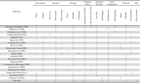
Table 1

Stochastic IRP Features

Reference

Time horizon Structure Routing Inventory policy

Inventory decisions

Fleet

composition Fleet size Risk

F in it e In fi n it e O n e -t o -o n e O n e-to -m a n y M an y -t o -m an y D ir e ct M u lt ip le C o n ti n u o u s M ax im u m l ev el ( M L ) o rd er -u p -t o -l ev el ( O U ) L o st s al es B ac k lo g g in g H o m o g e n eo u s H et er o g en e o u s S in g le M u lt ip le U n c o n st ra in ed R is k e v al u at io n

Federgruen and Zipkin (1984) √ √ √ √ √ √ √

Golden et al. (1984) √ √ √ √ √ √ √

Federgruen et al. (1986) √ √ √ √ √ √ √

Trudeau and Dror (1992) √ √ √ √ √ √ √

Minkoff (1993) √ √ √ √ √ √ √

Bard et al. (1998) √ √ √ √ √ √ √

Campbell et al. (1998) √ √ √ √ √ √ √

Qu et al. (1999) √ √ √ √ √ √ √

Berman and Larson (2001) √ √ √ √ √ √ √

Kleywegt et al. (2002) √ √ √ √ √ √ √

Ronen (2002) √ √ √ √ √ √ √

Adelman (2004) √ √ √ √ √ √ √

Kleywegt et al. (2004) √ √ √ √ √ √ √

Aghezzaf (2007) √ √ √ √ √ √ √

Hvattum and Løkketangen (2009) √ √ √ √ √ √ √

Hvattum et al. (2009) √ √ √ √ √ √ √

Huang and Lin (2010) √ √ √ √ √ √ √

Geiger and Sevaux (2011) √ √ √ √ √ √ √ √

Liu and Lee (2011) √ √ √ √ √ √ √

Solyalı et al. (2012) √ √ √ √ √ √ √

(5)

3. Problem Description and Model Formulation

Consider an inventory routing problem that contains one distributor and one type of product. The

distributor 0 delivers products to a set of N retailers over a given time horizon T. The product could be

sent from the distributor to the retailers at each period t T by a vehicle or a group of vehicles that have

the capacity of Q. In each period a quantity q_it of products is sent to the retailer i that have the demand

it

 . In some cases, we might face shortage of productq_it _it.

Our contribution to the literature is considering a risk measure in the model to control the cost that depot can afford. The cost consists of holding costs, carrying costs and backlogging cost. We consider a depot center or distributor who has financial limits. In other words, due to the capital limitations, we cannot satisfy every demand sent to our center. The risk measure changes the problem in three possible ways:

 The route structure can change.

 The amount of product sent to retailers can be determined.

 Controllable factors such as number of vehicles to satisfy the constraint related to risk measure

must be tunes.

The above-mentioned assumptions will be clarified after running the model. The assumptions are summarized as follows:

 The time horizon is finite and the period unit is day.

 The distributor has the capacity C0 and the retailers have the capacityCi i{1, 2, 3,...,N}.

 Retailer demand is stochastic with a known probability distribution function. The probability

distribution of demand _it i{1, 2, 3,...,N}and t{1, 2, 3,..., }T is assumed to be discrete.

 A fleet of homogeneous vehicles K is considered and each with capacity Q.

 Transportation cost of each vehicle (c_ij) on each period t is constant.

 The initial inventory for each distributor is considered.

 The model structure is one to many.

 The routing is multiple.

 Unmet demand is backlogged as back order.

 The model assumes holding cost for both distributors and retailers.

 Inventory policy is the maximum level (ML).

 Vehicles routes are cyclic, meaning that each the vehicle that travels its route returns back to the

distributor's node.

 The cost matrix is symmetric (C_ij C_ji).

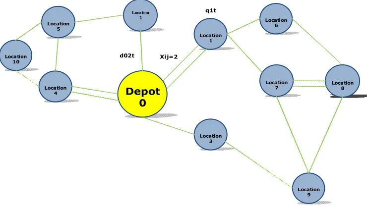
 The basic IRP is defined on a graph = ( , ) where V is the vertex set of nodes (V 

_

0,,n

_

)

and ( A{ ,

_

i j

_

: ,i jV i,  j}) is the set of arcs. Vertex indexed zero presents the supplier and

vertices '

V V {0} presents customers.

(6)

Depot 0

Location 3 Location

1

7 Location

6

Location 2

4 Location

5

Location

10 Xij=2

q1t

d02t

Fig. 1. IRP model structure

The parameters are described below:

Indices:

, {0,1, 2,..., }

i j N Indeces of customer and the depot, where 1, 2, 3,...,N are customer indices, and 0

demonstrates the depot node.

Time Period: t{1, 2, 3,..., }T Index of vehicles: k{1, 2, 3,..., }K

Parameters

it

h: Inventory holding cost in vertex i{0,1, 2,...,N} per period t{1, 2, 3,..., }T

i

C : Supplier and Customer holding capacity for i{0,1, 2,...,N}

it

I : Inventory level at the end of the period t i{0,1, 2,...,N}

,0 i

I : Inventory level at the beginning of period 1 for vertex i{0,1, 2,...,N}

it

 : Demand of customer i for each period t i{0,1, 2,...,N}; t{1, 2, 3,..., }T

Q: Capacity of vehicle for k{1, 2, 3,..., }K ij

c : Travel cost associated with arc ( , )i j it

 : Lost sale penalty for customer i in period t i{0,1, 2,...,N}; t{1, 2, 3,..., }T

it

b: Amount of product that is lost saled in customer i in period t i{0,1, 2,...,N},t{1, 2, 3,..., }T

( )

i

F t : Cumulative probability distribution function of demand

Decision variables

it

(7)

ijt

d : Demand quantity transported on arc ( , )i j in period t i{0,1, 2,...,N}; t{1, 2, 3,..., }T

ijt

x Number of the times that arc ( , )i j is traversed i in period t i{0,1, 2,...,N}; t{1, 2, 3,..., }T

Mathematical Model

0

1 1 1 1

0 0 1 0 1 1

min

T N K T N T N T N K

ij ijkt i it i it i kt

k t i k

t j i i t i t i

Z c x E h I E



b f x

                  _  _ _  _     







(1)

subject to

( it it )

P b VaR  (2)

1

( 1) ( 1)

it i t ikt it i t

K

it

k

I b I q  b



 

 



_

  i{1, 2,...,N},t{1, 2, 3,..., }T (3)

0 1 1 N K ikt k i q C   



t{1, 2, 3,..., }T (4)

,0 1

1 K

i ik i

k

I q C





_

 i{1, 2, 3,..., }N (5)

, 1 1 K

i t ikt i

k

I _ q C





_

 i{1, 2, 3,..., }N ,t{1, 2, 3,..., }T (6)

1 N ikt i q Q  



t{1, 2, 3,..., }T , k{1, 2, 3,..., }K (7)

0 1 1 K N jkt k j x K   

 

t{1, 2, 3,..., }T (8)

1 , 1,

n n

ijkt jikt

j j i j j i

x

   





i{1, 2, 3,...,N},k{1, 2, 3,...,K},

{1, 2, 3,..., }

t T (9)

0 1 1 N jkt j x  



t{1, 2, 3,..., }T ,k{1, 2, 3,...,K} (10)

1

1 N

ijkt j j i

x

 





i{1, 2, 3,...,N},k{1, 2, 3,...,K}

{1, 2, 3,..., }

t T (11)

it it

I M y i{1, 2, 3,...,N},t{1, 2, 3,..., }T (12)

(1 )

it it

b M y i{1, 2, 3,...,N},t{1, 2, 3,..., }T (13)

1 0,

( ).

K N

ikt jikt

k j j i

q x M

  



_{ }

i{1, 2, 3,...,N},k{1, 2, 3,...,K},

{1, 2, 3,..., }

t T (14)

( 1)

it jt ijkt

U U  N x N

, {1, 2, 3,..., },

i j N i j k{1, 2, 3,...,K}

{1, 2, 3,..., }

t T (15)

0

ikt

q  i{1, 2, 3,...,N},k{1, 2, 3,..., }K ,

{1, 2, 3,..., }

k K (16)

{ ,1}

, it 0

ijt

x y  i{1, 2, 3,...,N}k{1, 2, 3,..., }K (17)

0

it

b  i{1, 2, 3,...,N},t{1, 2, 3,..., }T (18)

0

it

I  i{1, 2, 3,...,N},t{1, 2, 3,..., }T (19)

(8)

each customer in each period should be less than the depot capacity. Constraints (5) ensure that every customer’s warehouse inventory capacity should be no less than its maximum inventory level in the period 1. Constraints (6) ensure that every customer’s warehouse inventory capacity should be no less

than its maximum inventory level in the period (t). Constraints (7) ensure that loading of each vehicle

in each period does not exceed respective capacities. Constraints (8) ensure that the number of vehicles used for delivery in each period does not exceed the number of vehicles. Constraints (9) ensure that the number of vehicles leaving from a customer or the depot is equal to that of arriving vehicles. Constraints (10) ensure that each vehicle can travel maximum once in each period. Constraints (11) ensure that each vehicle from current node can only travel to only another node. Constraint (12) and (13) ensure that at end of each period, each retailer cannot have both the inventory and back-order.

Constraint (14) is logical relationships between (q_ikt), (Xjikt). Constraints (15) avoid sub-tours for each

vehicle at each period. Finally, constraints (16) to (20) show the type of variables.

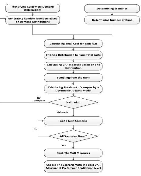
4. Simulation Optimization

The solution approach framework of this research is shown in Fig. 2. First, according to this figure, the probability distribution of the customers must be identified, and based on this, the customers’ demands is generated. The next step is to determine each scenario and number of runs that simulation must be implemented. Based on the scenarios, total cost for each run is calculated and then the probability distribution must be fitted to the total costs. In the next step, the VaR measure is identified based on significance level. For validating the solution procedure, some runs are randomly selected and supposing that their demands are deterministic, the exact solutions are obtained using the GAMS software. In this research, if the gap between the proposed and exact solution is less than 10% then the next scenario is simulated. Based on the VaR measure of all scenarios, scenarios are ranked and the best is chosen as the best solution of the problem.

Determining Scenarios

Generating Random Numbers Based on Demand Distributions Identifying Customers Demand

Distributions

Calculating Total Cost for each Run

Determining Number of Runs

Fitting a Distribution to Runs Total costs

Calculating VAR measure Based on The Distribution

Sampling from the Runs

Validation Calculating Total cost of samples by a

Deterministic Exact Model

Go to Next Scenario

Rank The VAR Measures All Scenarios Done?

Choose The Scenario With the Best VAR Measure at Preference Confidence Level

Not Adequate

Adequate

Yes No

(9)

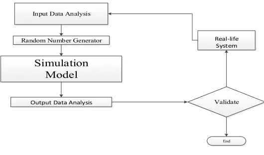
Since the Stochastic IRP is an NP- Hard problem, and with a VaR constraint becomes more complex, it is not possible to solve the large scale (and usually real-world cases) with an exact method. Simulation is a technique that measures and describes various characteristics of the bottom-line performance measure of a model when one or more values for the independent variables are uncertain. “Stochastic simulation optimization” (often shortened as simulation optimization) refers to stochastic optimization using simulation Specifically, the underlying problem is stochastic and the goal is to find the values of controllable parameters (decision variables) to optimize some performance measures of interest, which are evaluated via stochastic simulation, such as discrete-event simulation or Monte Carlo simulation (Fu, 2002; Fu et al., 2008). The act of obtaining the best decision under given circumstances is known as optimization.

Input Data Analysis

Random Number Generator

Output Data Analysis

Real-life System

Simulation Model

Validate

End

Fig. 3. Simulation Framework

Simulation allows one to specify a system accurately by using the logically complex, and often non-algebraic, variables and constraints. Complex and stochastic systems can therefore be modeled through simulation. While the development of the new technology has dramatically increased computational power, efficiency is still a big concern when using simulation for stochastic optimization problems. There are two important issues in the efficiency: (1) at the level of stochastic simulator, a large number of simulation replications must be performed in order to capture the randomness and obtain a sound statistical estimate at a specified level of confidence. (2) at the level of optimization, many design alternatives must be well evaluated via stochastic simulation in order to determine the best design or to iteratively converge to the optimal design.

The objective in simulation is to describe the distribution and characteristics of the possible values of

the bottom-line performance measure (

Y

) and the independent variables (X X₁, ₂,..., X_k). The idea

behind simulation is similar to the notion of playing out many what-if scenarios. The difference is that the process of assigning values to the cells in the spreadsheet that represent random variables is automated so that: (1) the values are assigned in a non-biased way, and (2) the spreadsheet software user is relieved of the burden of determining these values. With simulation, repeatedly and randomly,

sample values are generated for each uncertain input (X X₁, ₂,..., X_k) in the model, and then the result

value of our bottom-line performance measure

 

Y is computed. Then, the sample values of (

Y

) can be

used to estimate the true distribution and other characteristics of the performance measure (

Y

). For

(10)

possible outcomes, and a more precise idea about where the mean of the distribution is located. It is also known a way of determining how likely it is for the actual outcome to fall above or below some value.

4.1. Distribution fitting

The critical value (D__,_N) is pre-determined. After the data are collected, data can be plotted using a

histogram, and from the histogram or the problematic nature of the data, it can be determined which distribution is the most appropriate. Then, the parameters for that distribution can be estimated from the data using some principles such as Maximum Likelihood Estimation (MLE) or Minimum Squared Errors (MSE).

4.2. Goodness of fit test

After identifying the distribution, it is necessary to check how representative the fitted distribution is. It can be done by using either a heuristic approach or formal statistical tests. In the heuristic approach, a probability plot can be used, and from the plot, it can visually be determined if the distribution really fits well with the data. As for statistical tests, either chi-square tests or Kolmogorov–Smirnov tests can be used to check whether the distribution fits the data well. The idea of the Chi-Square Test is to compare the histogram with the probability mass function of the fitted distribution. The Kolmogorov– Smirnov Test focuses on the comparison of the distribution functions between the data and the fitted one.

4.2.1. Chi-square tests

This is an old but popular test. A chi-square test is considered as a formal comparison of a histogram with the probability density or mass function of the fitted distribution. The steps of doing the chi-square test are (Rao & Scott, 1981):

1. Draw the frequency histogram of the data.

2. Compute the probability content of each interval, p_i based on the fitted distribution.

3. Compute the expected frequency in each interval ˆf_i np_i where n is the total number of

observations.

4. Let f_i be that of observations in the interval. Compute the test statistic:

2

2 (ˆ )

ˆ

i i

f f

f

 

_



5. Determine the critical value at the level of significant  and 2

,

 

 with ddegrees of freedom,

where d = (number of intervals) − (number of estimated parameters)

6. Conclude that the data does not fit the distribution if the test statistics is greater than the

threshold.

4.2.2 Kolmogorov–Smirnov tests

Instead of grouping data in each interval as chi-square tests, Kolmogorov–Smirnov tests intend to

compare the empirical distribution function with the fitted distribution ( ˆF ). Kolmogorov Smirnov tests

do not require users to group data in any way and so no information is lost. The steps of doing the Kolmogorov-Smirnov test are (Massey Jr, 1951):

1. Rank the data from the smallest to the largest, i.e., R

_{ }

1 R

_{ }

2 ··· R

_

N

_

2. Compute:

1 1

1

ˆ ˆ

max ( ) , max ( )

i i

i N i N

i i

D F R D F R

N N

 

   



   

 _  _  _  _

(11)

3. ComputeD max D



, D



,

4. Determine the critical value, D__,N,

5. Step 5. The data does not fit the distribution ifD>D_,N.

4.3. Random Number and Variables Generation

When running a simulation, it is necessary to generate random numbers that follow some certain distributions for capturing the system’s stochastic behaviors, such as service times or customer inter-arrival times. In computer simulation, a procedure to generate a sequence of numbers is used in order to behave similarly to the random number, which are called pseudo random numbers. The process that generates these numbers is called random number generator.

In order to generate numbers fitting to a certain distribution, it is needed to first generate a number following a uniform distribution between zero and one, and then some random variable generation methods are used to transform the uniform random number into a random number that follows the required distribution.

4.4.Output Analysis

Output analysis aims at analyzing the data generated by simulation, and estimates the performance of the system. Since the simulation is stochastic, multiple simulation replications must be performed in order to have a good estimate. The required number of simulation replications depends on the uncertainties of the simulation output. In output analysis, it is useful to look into ways to analyze the simulation output and then decide how long each simulation should be run and how many times is needed to replicate the simulation.

4.5.Verification and Validation

After the simulation model is constructed, it must be verified and validated to ensure it represents the actual system. Verification refers to check the model to see whether the conceptual model is accurately coded into a computer program while validation involves with checking the model to see whether it sufficiently represents the actual system so that the objectives of the simulation study can be achieved. The purpose of validation is to compare the behavior of the simulation model to the real system. However, for validation, it should be noticed that although no model is completely representative of the system under study, some models could be useful. Hence, it is always important to know the objective of the simulation study so that the simulation model is able to help to achieve the proposed objective. There are two different types of tests, which can be used for validation.

Subjective test: It is also known as a qualitative test. People who are knowledgeable on one or more aspects of the system should be involved, and let them to check if the model is reasonable.

Objective test: Is also known as a quantitative test. Statistical tests are used to compare some aspects of the system data set with the model data set. The model assumptions must be validated, and then compare the model input-output relationships to corresponding input-output relationships in the real system. Test 2 is utilized in this study.

5. Experimental results

In this section, some computational examples are presented to illustrate possible applications of the

proposedmodel for considering the risk of lack of capital in an IRP. In this section some computational

(12)

Table 2

Customer Demand Distributions

Customer Lower Upper Mean StdVar

C1 100 200 150 28.86

C2 75 145 110 20.2

C3 250 330 190 23.09

C4 180 230 205 14.43

C5 210 225 217.5 4.33

We run each scenario for over 100 times. Each run contains seven working days (T7). Considering

this, all surplus and shortage demand until the seventh day are retained and then for next run the history

of the system is erased (i.e., surplus and shortage demand in t0 (beginning of the period) is equal to

zero). Performing these runs, the cost of each run is calculated. It should be noticed that in a scenario cost of transportation and vehicle fixed cost don’t change, because the transportation cost is dependent on the route structure and qi and since neither of them change it remains fixed in every run. The cost matrix for transportation is as Table 3.

Table 3

Transportation Cost Matrix

j

i 0 1 2 3 4 5

0 0 728 324 756 416 800

1 728 0 704 348 752 388

2 324 704 0 448 332 708

3 756 348 448 0 228 252

4 416 752 332 228 0 276

5 800 388 708 252 276 0

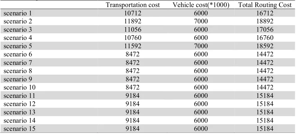
The fixed cost of vehicles is considered 1000 unit. So the routing cost that contains a fixed cost of vehicles and the cost of transportation is calculated. The Table 4

Total Transportation Cost for each Scenario (first 15) shows these costs for all scenarios.

Table 4

Total Transportation Cost for each Scenario (first 15)

Transportation cost Vehicle cost(*1000) Total Routing Cost

scenario 1 10712 6000 16712

scenario 2 11892 7000 18892

scenario 3 11056 6000 17056

scenario 4 10760 6000 16760

scenario 5 11592 7000 18592

scenario 6 8472 6000 14472

scenario 7 8472 6000 14472

scenario 8 8472 6000 14472

scenario 9 8472 6000 14472

scenario 10 8472 6000 14472

scenario 11 9184 6000 15184

scenario 12 9184 6000 15184

scenario 13 9184 6000 15184

scenario 14 9184 6000 15184

(13)

Table 5

Total Transportation Cost for each Scenario (second 15)

Transportation cost Vehicle cost(*1000) Total Routing Cost

scenario 16 10052 7000 17052

scenario 17 10052 7000 17052

scenario 18 10052 7000 17052

scenario 19 10052 7000 17052

scenario 20 10052 7000 17052

scenario 21 11580 6000 17580

scenario 22 11580 6000 17580

scenario 23 11580 6000 17580

scenario 24 11580 6000 17580

scenario 25 11580 6000 17580

scenario 26 12208 6000 18208

scenario 27 12208 6000 18208

scenario 28 12208 6000 18208

scenario 29 12208 6000 18208

scenario 30 12208 6000 18208

For each period (day), the back order cost or holding cost is also calculated and added to transportation cost. The back order and holding cost per unit is as Table 6.

Table 6

Holding cost and Backorder Cost for Customer i

Customer 1 2 3 4 5

h 12 15 14 18 19

pi 20 8 22 16 7

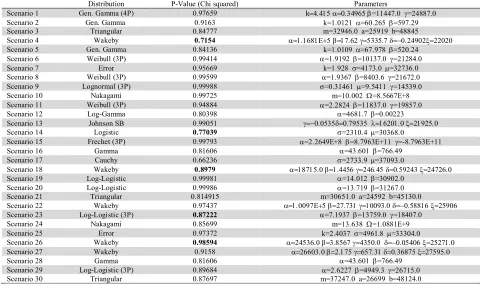
By calculating all of these costs, a number is dedicated to every run. So for each run total cost is considered. These total costs follow a distribution that should be identified. Thorough a chi-square test explained in previous section, the best distribution of total costs is fitted. Different distributions can be obtained from the chi-square test. The distributions for the example scenarios are shown in Table 7.

Table 7

Distribution for scenarios total costs

Distribution P-Value (Chi squared) Parameters

Scenario 1 Gen. Gamma (4P) 0.97659 k=11447.0 =24887.0

Scenario 2 Gen. Gamma 0.9163 k=1.0121 =60.265 =597.29

Scenario 3 Triangular 0.84777 m=32946.0 a=25919 b=48845

Scenario 4 Wakeby 0.7154 

Scenario 5 Gen. Gamma 0.84136 k=1.0109 =67.978 =520.24

Scenario 6 Weibull (3P) 0.99414 =1.9192 =10137.0 =21284.0

Scenario 7 Error 0.95669 k=1.928 =4173.0 =32736.0

Scenario 9 Lognormal (3P) 0.99988 =0.31461 =9.5411 =14539.0

Scenario 10 Nakagami 0.99725 m=10.002 =8.5667E+8

Scenario 12 Log-Gamma 0.80398 =4681.7 =0.00223

Scenario 13 Johnson SB 0.99051 

Scenario 14 Logistic 0.77039 =2310.4 =30368.0

Scenario 15 Frechet (3P) 0.99793 =2.2649E+8 =8.7963E+11 =-8.7963E+11

Scenario 16 Gamma 0.81606 =43.601 =766.49

Scenario 17 Cauchy 0.66236 =2733.9 =37093.0

Scenario 18 Wakeby 0.8979 

Scenario 19 Log-Logistic 0.99981 =14.012 =30902.0

Scenario 20 Log-Logistic 0.99986 =13.719 =31267.0

Scenario 21 Triangular 0.814915 m=30651.0 a=24592 b=45130.0

Scenario 22 Wakeby 0.97437 

Scenario 23 Log-Logistic (3P) 0.87222 =7.1937 =13759.0 =18407.0

Scenario 24 Nakagami 0.85699 m=13.638 =1.0881E+9

Scenario 25 Error 0.97372 k=2.4037 =4961.8 =33304.0

Scenario 26 Wakeby 0.98594 

Scenario 27 Wakeby 0.9158 

Scenario 28 Gamma 0.81606 =43.601 =766.49

Scenario 29 Log-Logistic (3P) 0.89684 =2.6227 =4949.3 =26715.0

(14)

Note that the colored cells in P-Value column are the ones that the distribution related to them is chosen through a Kolmogorov Smirnov test. In the state, where chi square test is not reliable enough, hence, for choosing the best distribution Kolmogorov Smirnov test is utilized. After the distribution of each scenario is identified. VaR measure is calculated considering four different significance levels. The significance levels considered are 0.005, 0.025, 0.05, and 0.10. The significance levels may change by user preference.

The scenarios are designed by best possible routes and different set of q_i . Each q_iis calculated based

on the holding cost and back order cost. The logic behind determining each q_iis that if the holding cost

of a customer is bigger than its backorder cost (h_i p_i ) a certain ratio of standard deviation is subtracted to the mean of that customer demand. Otherwise if the holding cost is lower than the back

order cost (h_i p_i) a certain ratio of standard deviation is added to the customer demand. This makes

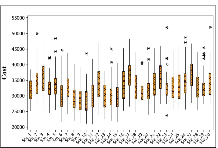
sure that the system bear lower cost. Table 8 and Table 9 show the results of 30 scenarios. For each significance level the rank of each scenario is calculated and regard to manager preference for significance level the best scenario is chosen. Fig. 4 shows the box plot for all scenarios that can be used to recognize best scenarios especially when the VaR is not important.

Sce_ 30 Sce_ 29 Sce_ 28 Sce_ 27 Sce_ 26 Sce_ 25 Sce_ 24 Sce_ 23 Sce_ 22 Sce_ 21 Sce_ 20 Sce_ 19 Sce_ 18 Sce_ 17 Sce_ 16 Sce_ 15 Sce_ 14 Sce_ 13 Sce_ 12 Sce_ 11 Sce_ 10 Sce_ 9 Sce_ 8 Sce_ 7 Sce_ 6 Sce_ 5 Sce_ 4 Sce_ 3 Sce_ 2 Sce_ 1 55000 50000 45000 40000 35000 30000 25000 20000 C o st

Fig. 4. Total Cost Box Plots for each Scenario

Table 8

Results of Simulation Optimization for First 15 Scenarios

Route Structure qi VAR(0.995) VAR(0.975) VAR(0.95) VAR(.9)

Value Rank Value Rank Value Rank Value Rank

Scenario 1 1.2.3-4-5 qi=mean(i) 40008 2 38381 5 37457 6 36359 8

Scenario 2 1.2.3-4-5 qi=mean(i)+or-0.5(STDVar) 46539 20 43300 21 41745 21 39966 22

Scenario 6 3.1.2-4.5 qi=mean(i) 45449 16 41295 13 39237 12 36938 12

Scenario 7 3.1.2-4.5 qi=mean(i)+or-0.5(STDVar) 43608 8 40954 12 39607 15 38065 15

Scenario 11 5.2-3-4-1 qi=mean(i) 44433 11 40828 18 39001 10 36916 11

Scenario 12 5.2-3-4-1 qi=mean(i)+or-0.5(STDVar) 50025 27 45451 13 43284 25 40921 25

(15)

Table 9

Results of Simulation Optimization for Second 15 Scenarios

Route Structure qi VAR(0.995) VAR(0.975) VAR(0.95) VAR(.9)

Value Rank Value Rank Value Rank Value Rank

Scenario 16 1.2-3-4.5 qi=mean(i) 47890 24 44044 22 42157 6 40048 23

Scenario 17 1.2-3-4.5 qi=mean(i)+or-0.5(STDVar) 47045 21 45710 27 44711 30 43297 30

Scenario 21 3-2.1.4.5 qi=mean(i) 43911 9 42403 19 41274 19 39677 20

Scenario 22 3-2.1.4.5 qi=mean(i)+or-0.5(STDVar) 45947 18 44748 24 43761 28 42278 28

Scenario 26 5-2.3-1.4 qi=mean(i) 51674 29 46181 29 43664 27 41050 26

Scenario 27 5-2.3-1.4 qi=mean(i)+or-0.5(STDVar) 50620 28 44978 25 43406 26 42129 27

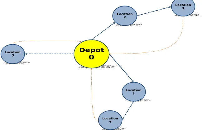
As it is clear from the, in 0.9 significance level, the scenario number 30 is the best scenario. For 0.95 and 0.975 significance level, again scenario 30 with 5-2.3-1.4 route shape shown in figure 5 is the best among all scenarios. However, for 0.995 significance level, the scenario number 13 comes to top.

Fig. 5. Route Structure for Optimized Scenarios (Scenario 30)

According to Fig. 5, the orange lines are return routs that are the routs each vehicle travels for coming back to the depot. To validate the simulation random runs are chosen from each scenario and considering the demand related to that run is deterministic it is solved through an exact model represented in problem definition section. If the result of two answers is not deviated more than 10 percent then the scenario is accepted. The table below shows some example of validation for the problem we solved.

(16)

Table 10

Validation Table

Scenario 10 Features Run number

22 35 38

Exact method Total cost 20076 20405 20164

Processing time 53.27 mins 55.39 mins 51.01 mins

Simulation optimization Total cost 21522 22309 21182

Processing time 19 sec 19 sec 19 sec

Relative gap 7.2% 8.3% 8.9%

6. Conclusion and Future Research

Inventory Routing Problem addresses the issue of coordinating inventory replenishment policies and distribution plans in a cost effective manner. More precisely, the IRP integrates inventory and distribution aspects in the same planning process. Considering the risk of allocating capital to this matter has been quite an issue to the managers. In this study a model has been proposed that deals with the risk of allotting too much capital in an IRP with stochastic demand. A VaR measure has been considered to be able to model the risk. This measure acts like a constraint in the model and does not let the cost of an inventory routing exceeds from VaR in a known significance level. To solve the model, a simulation optimization approach has been applied. The approach helps dealing with uncertainty of demand. To validate the simulation optimization some samples randomly are chosen and have been solved thorough exact method. The results of validation in experimental results showed the simulation optimization approach is quite adequate.

For further works, one may consider the problem by heterogeneous vehicles. Also, modeling a dynamic stochastic inventory routing problem (DSIRP) while considering the risk can be an appropriate field of study. For more efficient simulation optimization, one can make a pre-selection for scenarios.

References

Aviv, Y., & Federgruen, A. (1998). The operational benefits of information sharing and vendor

managed inventory (VMI) programs. Olin School of Business Working Paper.

Adelman, D. (2004). A price-directed approach to stochastic inventory/routing. Operations Research,

52(4), 499-514.

Aghezzaf, E. H. (2008). Robust distribution planning for supplier-managed inventory agreements when

demand rates and travel times are stationary. Journal of the Operational Research Society, 59(8),

1055-1065.

Archetti, C., Bertazzi, L., Hertz, A., & Speranza, M. G. (2012). A hybrid heuristic for an inventory

routing problem. INFORMS Journal on Computing, 24(1), 101-116.

Archetti, C., Bertazzi, L., Laporte, G., & Speranza, M. G. (2007). A branch-and-cut algorithm for a

vendor-managed inventory-routing problem. Transportation Science, 41(3), 382-391.

Bard, J. F., & Nananukul, N. (2009). Heuristics for a multiperiod inventory routing problem with

production decisions. Computers & Industrial Engineering, 57(3), 713-723.

Bard, J. F., Huang, L., Jaillet, P., & Dror, M. (1998). A decomposition approach to the inventory

routing problem with satellite facilities. Transportation science, 32(2), 189-203.

Bent, R. W., & Van Hentenryck, P. (2004). Scenario-based planning for partially dynamic vehicle

routing with stochastic customers. Operations Research, 52(6), 977-987.

Berman, O., & Larson, R. C. (2001). Deliveries in an inventory/routing problem using stochastic

dynamic programming. Transportation Science, 35(2), 192-213.

Bertazzi, L., Bosco, A., Guerriero, F., & Laganà, D. (2013). A stochastic inventory routing problem

with stock-out. Transportation Research Part C: Emerging Technologies, 27, 89-107.

Bertazzi, L., Paletta, G., & Speranza, M. G. (2002). Deterministic order-up-to level policies in an

(17)

Cáceres-Cruz, J., Juan, A. A., Bektas, T., Grasman, S. E., & Faulin, J. (2012, December). Combining Monte Carlo simulation with heuristics for solving the inventory routing problem with stochastic

demands. In Proceedings of the Winter Simulation Conference (p. 274). Winter Simulation

Conference.

Campbell, A., Clarke, L., Kleywegt, A., & Savelsbergh, M. (1998). The inventory routing problem. In

Fleet management and logistics (pp. 95-113). Springer US.

Campbell, A. M., & Savelsbergh, M. W. (2004). A decomposition approach for the inventory-routing

problem. Transportation Science, 38(4), 488-502.

Chen, X., Sim, M., Simchi-Levi, D., & Sun, P. (2007). Risk aversion in inventory management.

Operations Research, 55(5), 828-842.

Chen, Y. M., & Lin, C. T. (2009). A coordinated approach to hedge the risks in stochastic

inventory-routing problem. Computers & Industrial Engineering, 56(3), 1095-1112.

Coelho, L. C., Cordeau, J. F., & Laporte, G. (2013). Thirty years of inventory routing. Transportation

Science, 48(1), 1-19.

Federgruen, A., Prastacos, G., & Zipkin, P. H. (1986). An allocation and distribution model for

perishable products. Operations Research, 34(1), 75-82.

Federgruen, A., & Zipkin, P. (1984). A combined vehicle routing and inventory allocation problem.

Operations Research, 32(5), 1019-1037.

Fu, M. C. (2002). Optimization for simulation: Theory vs. practice. INFORMS Journal on Computing,

14(3), 192-215.

Fu, M. C., Chen, C. H., & Shi, L. (2008, December). Some topics for simulation optimization. In

Proceedings of the 40th Conference on Winter Simulation (pp. 27-38). Winter Simulation Conference.

Geiger, M. J., & Sevaux, M. (2011). Practical inventory routing: A problem definition and an

optimization method. arXiv preprint arXiv:1102.5635.

Golden, B., Assad, A., & Dahl, R. (1984). Analysis of a large scale vehicle routing problem with an

inventory component. Large Scale Systems, 7(2-3), 181-190.

Huang, S. H., & Lin, P. C. (2010). A modified ant colony optimization algorithm for multi-item

inventory routing problems with demand uncertainty. Transportation Research Part E: Logistics

and Transportation Review, 46(5), 598-611.

Hvattum, L. M., & Løkketangen, A. (2009). Using scenario trees and progressive hedging for

stochastic inventory routing problems. Journal of Heuristics, 15(6), 527-557.

Hvattum, L. M., Løkketangen, A., & Laporte, G. (2007). A branch‐and‐regret heuristic for stochastic

and dynamic vehicle routing problems. Networks, 49(4), 330-340.

Hvattum, L. M., Løkketangen, A., & Laporte, G. (2009). Scenario tree-based heuristics for stochastic

inventory-routing problems. INFORMS Journal on Computing, 21(2), 268-285.

Kleywegt, A. J., Nori, V. S., & Savelsbergh, M. W. (2002). The stochastic inventory routing problem

with direct deliveries. Transportation Science, 36(1), 94-118.

Kleywegt, A. J., Nori, V. S., & Savelsbergh, M. W. (2004). Dynamic programming approximations for

a stochastic inventory routing problem. Transportation Science, 38(1), 42-70.

Korsvik, J. E., Fagerholt, K., & Laporte, G. (2010). A tabu search heuristic for ship routing and

scheduling. Journal of the Operational Research Society, 61(4), 594-603.

Li, F., Golden, B., & Wasil, E. (2007). A record-to-record travel algorithm for solving the

heterogeneous fleet vehicle routing problem. Computers & Operations Research, 34(9), 2734-2742.

Liu, S. C., & Lee, W. T. (2011). A heuristic method for the inventory routing problem with time

windows. Expert Systems with Applications, 38(10), 13223-13231.

Luciano, E., Peccati, L., & Cifarelli, D. M. (2003). VaR as a risk measure for multiperiod static

inventory models. International Journal of Production Economics, 81, 375-384.

Massey Jr, F. J. (1951). The Kolmogorov-Smirnov test for goodness of fit. Journal of the American

statistical Association, 46(253), 68-78.

Minkoff, A. S. (1993). A Markov decision model and decomposition heuristic for dynamic vehicle

(18)

Popović, D., Vidović, M., & Radivojević, G. (2012). Variable neighborhood search heuristic for the

inventory routing problem in fuel delivery. Expert Systems with Applications, 39(18), 13390-13398.

Qu, W. W., Bookbinder, J. H., & Iyogun, P. (1999). An integrated inventory–transportation system

with modified periodic policy for multiple products. European Journal of Operational Research,

115(2), 254-269.

Rao, J. N. K., & Scott, A. J. (1981). The analysis of categorical data from complex sample surveys:

chi-squared tests for goodness of fit and independence in two-way tables. Journal of the American

Statistical Association, 76(374), 221-230.

Ronen, D. (2002). Marine inventory routing: Shipments planning. Journal of the Operational Research

Society, 108-114.

Schedl, M., & Strausss, C. (2011, June). A periodic routing problem with stochastic demands. In

Complex, Intelligent and Software Intensive Systems (CISIS), 2011 International Conference on

(pp. 350-357). IEEE.

Solyali, O., Cordeau, J. F., & Laporte, G. (2012). Robust inventory routing under demand uncertainty.

Transportation Science, 46(3), 327-340.

Talbi, E. G. (2002). A taxonomy of hybrid metaheuristics. Journal of heuristics, 8(5), 541-564.

Tirado, G., Hvattum, L. M., Fagerholt, K., & Cordeau, J. F. (2013). Heuristics for dynamic and

stochastic routing in industrial shipping. Computers & Operations Research, 40(1), 253-263.

Trudeau, P., & Dror, M. (1992). Stochastic inventory routing: Route design with stockouts and route

failures. Transportation Science, 26(3), 171-184.

Wu, J., Li, J., Wang, S., & Cheng, T. C. E. (2009). Mean–variance analysis of the newsvendor model

with stockout cost. Omega, 37(3), 724-730.

Yang, L., Gao, C., Chen, K., & Li, J. (2007). Downside risk-aversion analysis for a single-stage

newsvendor problem. Wuhan University Journal of Natural Sciences, 12(2), 198-202.

Zhang, D., Xu, H., & Wu, Y. (2009). Single and multi-period optimal inventory control models with