Tackling Temporal Effects in
Automatic Document Classification
Thiago Salles1⋆, Thiago Cardoso1, Vitor Oliveira1, Leonardo Rocha2, Marcos Andr´e Gon¸calves1
1 Dep. de Ciˆencia da Computa¸c˜ao - Universidade Federal de Minas Gerais (UFMG)
Av. Antˆonio Carlos 6627 - ICEx - 31270-010 Belo Horizonte, Brasil {tsalles,thiagon,vitorco,mgoncalv}@dcc.ufmg.br
2 Dep. de Ciˆencia da Computa¸c˜ao - Universidade Federal de S˜ao Jo˜ao Del Rei (UFSJ)
Pc. Dr. Augusto Chagas Viegas 17 - DCOMP - 36300-088 S˜ao Jo˜ao Del Rei, Brasil [email protected]
Abstract. Automatic Document Classification (ADC) has become an important research topic due the rapid growth in volume and complexity of data produced nowadays. ADC usually employs a supervised learning strategy, where we first build a classification model using pre-classified documents and then use it to classify unseen documents. One major challenge in building classifiers has to do with the temporal evolution of the characteristics of the dataset (a.k.a temporal effects). However, most of the current techniques for ADC does not consider this evolution while building and using the classification models. Recently we have proposed temporally-aware algorithms for ADC in order to properly handle these temporal effects. Despite of the their effectiveness, the temporally-aware classifiers have a major side effect of being nat-urally lazy, since they need to know the creation time of the test document to build the model. Such lazy property incurs in a potentially high test phase runtime and brings a critical scalability issue that may make these classifiers infeasible to handle large volumes of data, such as the Web and very large digital libraries. This work aims at addressing the following challenge: can we deal with the temporal effects in some entirely off-line setting, reducing the test phase runtime and without compromising its effectiveness due to varying data distributions? We propose to address this question by tackling the temporal effects from a data engineering perspective. We devise a pre-processing—classifier independent—step able to moving all the overhead of considering the temporal effects to an off-line setting, called Cascaded Temporal Smoothing (CTS). The CTS consists of a controlled data oversampling strategy which aims at smoothing the observed temporal ef-fects in the data distribution. This new training set can be used by any traditional classifier in a way that produces similar effectiveness as the lazy temporally-aware classifiers but not incurring in any overhead at test phase. As our experimental evaluation shows, the use of CTS before learning a traditional Na¨ıve Bayes classifier was able to improve classification effectiveness in two real datasets (gains up to 5.00% in terms of MacroF1) exhibiting scalability properties not present
in the lazy temporally-aware classifiers, guaranteeing its practical applicability in large classification problems.
Categories and Subject Descriptors: H.2.8 [Database Applications]: Data mining
General Terms: Algorithms, Experimentation
Keywords: automatic document classification, temporal effects, oversampling
1. INTRODUCTION
Automatic Document Classification (ADC) plays an important role in many information retrieval ap-plications. Basically, the ADC goal is to create effective models to automatically associate documents
⋆Corresponding author.
This research is partially funded by the MCT/CNPq/CT-INFO project InfoWeb (grant number 55.0874/2007−0), by InWeb – The National Institute of Science and Technology for the Web (MCT/CNPq/FAPEMIG grant number 573871/2008−6), and by the authors’ individual research grants from FAPEMIG, FINEP and CNPq.
with semantically meaningful categories. With the rapid growth in volume and complexity of data produced nowadays, this task has become essential for a variety of applications such as ad-matching systems [Rajan et al. 2010], news recommendation [Chiang and Chen 2004] and spam filtering [Fdez-Riverola et al. 2007].
Similarly to other machine learning techniques, ADC usually follows a supervised learning approach: a set of already classified documents (training set) is employed for creating a classification model. Once built, the model is used for labeling a new set of unclassified documents (test set). A fundamental as-sumption of the majority of ADC algorithms is that the data used to learn a model are random samples independently and identically distributed (i.i.d.) from a stationary distribution that governs the test data. However, in many (perhaps most) real-world classification problems, the training data may not be randomly drawn from the same distribution as the test data (to which the classifier will be applied).
Recently, in [Mour˜ao et al. 2008] the authors have distinguished three different temporal effects that may have a significant impact on ADC algorithms. More specifically, theterm distribution variation
effect refers to changes in the term’s representativeness with respect to the classes as time goes by (i.e., the observed variations over time in the strength of term-class relationships). The second effect,class
distribution variation, accounts for the impact of the temporal evolution on the relative frequencies
of the classes. Finally, theclass similarity variation considers how the similarity between classes, as a function of the terms that occur in their documents, changes over time. Therefore, as the authors showed, the design of classification models that account for the temporal dynamics of data is a critical challenge to be tackled. Neglecting this issue potentially leads to less effective classifiers as assumptions made when the model is built (i.e., learned) may no longer hold due to the temporal effects.
In [Salles et al. 2010], the authors proposed a strategy to incorporate temporal information directly into document classifiers, aiming at improving their effectiveness by handling data with varying dis-tributions. Such strategy is based on the evolution of the term-class relationship over time, captured by a metric ofdominance. In that work, the authors developed a statistically well founded way to de-termine thetemporal weighting function(TWF) according to the characteristics of the target dataset to which the classifier will be applied. Having defined the TWF, they also proposed two strategies to incorporate this function to ADC algorithms, both following a lazy instance-weighting classification approach. In these strategies, the weights assigned to each training document depend on the notion of a temporal distanceδ, defined as the difference between the time of creationpof a training document and a reference time pointpr (i.e., the creation time of test document). One drawback of these lazy algorithms is that they postpone the construction of a classification model until the classifier receives the test document, in order to assess its creation time. Thus, for each test document, a specific clas-sification model is learned. In fact, learning a clasclas-sification model is a rather costly procedure and, since it is performed for each test instance, the scalability of the temporally-aware classifiers becomes compromised (i.e., they do not handle large datasets efficiently). This scenario poses the following challenge: can the temporal effects be addressed in some entirely off-line setting (instead of a lazy learning setting), ultimately contributing to a scalable classification system without being negatively affected by varying data distributions?
improve the class’ representativity while minimizing the observed variations in the data distribution. The main motivation behind CTS is that, as reported in [Salles 2011], a large presence of the temporal effects in the training data can significantly degrade the classification effectiveness, motivating us to devise a pre-processing step able to reduce these variations in the training data characteristics (by propagating documents through the time line) as a way to improve classification effectiveness. Our hope is that, with a higher quality training set (i.e., with the temporal effects smoothed out), a regular (traditional) classifier may be able to provide more accurate predictions.
Unlike previously proposed temporally-aware classifiers, which demand a lazy classification ap-proach, the strategy proposed here handles the temporal effects entirely off-line. This means that, using CTS, the test phase runtime becomes independent on the training set size while maintaining the classifier robust to the temporal effects. Moreover, since the data is preprocessed before the actual classification, the time required to perform CTS is spent only once for any classifier used. Both aspects directly contribute to the scalability of the solution. Finally, this preprocessing step is independent of the classifier selected for the ADC, as it does not impose any constraints regarding which classifier should be used to make the predictions and does not involve any modifications to existing classi-fiers.1 Although this data engineering approach may incur in some additional time due to this new pre-processing step, as our experimental evaluation will show, this is still worthwhile. The increase in training time is indeed very small when compared with the drastic reduction achieved in the test run-time. That is, CTS increases the classifier throughput in terms of the number of classified documents per time unit, preserving the classification effectiveness in face of the temporal effects. This makes the CTS a very effective and robust solution to ADC in face of large datasets with varying distributions.
We evaluate our proposal considering two real and large textual datasets, namely ACM-DL and MEDLINE. We evaluate the traditional Na¨ıve Bayes classifier trained with the new training set pro-duced by CTS contrasting it with the Temporally-Aware Na¨ıve Bayes.2 Our experimental evaluation shows that the use of CTS before learning the classifier achieved gains up to 5.00% in terms of MacroF1 for the ACM-DL dataset when compared to a traditional classifier learned from the original training set, while being statistically tied with the temporally-aware classifier. Moreover, in the case of MED-LINE, using the training set augmented by CTS achieved gains to up to 5.13% in MacroF1 when compared to a Na¨ıve Bayes classifier learned from the original training set, and achieved a marginal (but statistically significant) gain of 2.75% when compared to the temporally-aware classifier. Fur-thermore, we show that our CTS approach exhibits scalability properties not presented by the lazy temporally-aware classifiers, guaranteeing its practical applicability in large classification problems.
The remainder of this work is organized as follows: Section 2 discusses some related work. Section 3 describes our proposed CTS algorithm, as well as a probabilistic analysis regarding its properties. In Section 4 we evaluate our approach and, finally, in Section 5 we conclude and discuss future work.
2. RELATED WORK
While ADC is a widely studied topic, the analysis of the impact caused by the temporal aspects has only started in the last decade. As stated before, a recent effort was made in order to characterize this problem and provide valuable insights to the development of temporally robust classifiers. In [Mour˜ao et al. 2008], the authors present a qualitative analysis regarding the existence of three main temporal effects, which are, in fact, manifestations of the drifting patterns first analyzed by [Forman 2006]. Further effort was made by [Salles 2011] in order to quantitatively characterize these effects using a factorial experimental design. That work advances the qualitative analysis reported in [Mour˜ao et al. 2008] byquantifyingto what extent each temporal effect influences three real datasets and their
1Although not exploited in this work, our approach also allows us to explore other state-of-the-art algorithms such as
SVM, whose any lazy temporally-aware version would be infeasible.
negative impact to the effectiveness of four widely used ADC algorithms. The main findings are that the presence of temporal effects in the data used to learn a classifier really do negatively impact the classification effectiveness, motivating us to develop techniques to smooth out such effects.
Proposed methods that attempt tominimize the impact of temporal effects in ADC can be cat-egorized in two broad areas, namely, adaptive document classification and concept drift. Adaptive document classification [Cohen and Singer 1999] embodies a set of techniques to deal with changes in the underlying data distribution in order to improve the effectiveness of classifiers through incremental and efficient adaptation of the classification models. On the other hand, concept (or topic) drift [Tsym-bal 2004] groups techniques in which the classifier is completely retrained according to some instance selection or weighting method. It comprises most of the recent efforts in dealing with temporal aspects and data streams with changing distributions, from a wide domain of applications like textual classifi-cation [Wang et al. 2010], recommendation systems based in collaborative filtering [Koren 2010] and others. A number of previous studies fall into this category. In [Klinkenberg and Joachims 2000] a slid-ing window with examples sufficiently “close” to the current target concept has its size automatically adjusted in order to minimize the estimated generalization error. The method proposed in [ˇZliobait˙e 2009] builds the classification model using training instances which are close to the test in terms of both time and space. In [Klinkenberg 2004] different approaches are used such as adaptive time window on the training data and selection or weighting of representative training examples for model construction. [Widmer and Kubat 1996] describe a set of algorithms that react to concept drift in a flexible way and can take advantage of situations of recurring contexts. The main idea of these algorithms is to keep only a window of currently trusted examples and hypothesis, and store concept descriptions in order to reuse them if a previous context reappears. [Rocha et al. 2008] introduce the concept oftemporal context, de-fined as a subset of the dataset that minimizes the impact of temporal effects in the performance of clas-sifiers. These temporal contexts are used to sample the training examples for the classification process, discarding instances that are considered to be outside this context. An algorithm, namedChronos, to identify these contexts based on the stability of the terms in the training set is also proposed.
Instance selection approaches may be considered too rigid since they may miss valuable information laying outside of the window. This motivates the use of instance weighting approaches. Following this direction, in [Salles et al. 2010] the temporal information is incorporated to document classi-fiers based on the evolution of term-class relationship over time, which is captured by a metric of
dominance [Rocha et al. 2008]. Atemporal weighting function (TWF) is defined for a given dataset
by means of a series of statistical tests aimed at determining the TWF’s expression. A curve fitting procedure is then employed to determine its parameters. The discovered TWF is then incorporated to ADC algorithms, by means of two different strategies, namely, “TWF in documents” and “TWF in scores”. The first strategy weights each training document by the TWF according to its temporal dis-tance to the test documentd′. The second strategy considers the “scores” produced by the traditional classifiers learned from a training set whose documents’ class is transformed to a new derived class hc, pi, wherecis the actual document class andpdenotes its creation point in time. The test document d′ is then classified by such traditional classifier, which generates scores for eachhc, pi. The obtained scores for each derived class are aggregated through a weighted sum, where the weights correspond to the TWF considering the temporal distance betweenpand the creation time of d′. Both strategies have one common property: they follow a lazy classification approach, since the classification model is only defined after discovering the creation time of the test document.
model is applied for predicting the test document and the resulting prediction is appended to both the test and training data, in the form of a new binary feature. This augmented test document is then classified by the next model (p1), learned from the training set with augmented feature space, and its output is also appended to the documents. This cascaded procedure proceeds until the test document is classified with the model associated to the target domain (pn). In [Zhao and Hoi 2010], the authors also propose a classification strategy based on the transfer learning paradigm, however considering an online learning [Crammer et al. 2006] task. In this case, transfer learning is used to combine one previously built model with an online learning model, in order to take advantage of data whose distribution may not be the same as the distribution currently observed. The proposed Online Transfer Learning (OTL) algorithm uses this combination in order to learn from data that potentially comes from a distinct distribution (for example, due to concept drift) increasing both the initial performance of the online classifier and its asymptotic effectiveness.
All the previously described solutions incur in overhead at the test phase of the classification task. Sliding windows depends on the test data to define its size: fast variations on the test set reduces the windows size, whereas gradual variations increase its size. For each window configuration, there exists an overhead of determining if its size is (near-)optimal, ultimately increasing the test phase runtime. Instance weighting strategies are naturally lazy since the model becomes dependent on the instance weights which, by their own, depend on the temporal distance between test and training samples. The TIX method propagates the classifiers’ predictions regarding each point in time prior to the test’s creation time (using binary features), thus incurring in overhead at test phase. The OTL algorithm, on the other hand, moves all calculations to the test phase (online learning). Differently from the previously described methods, the strategy proposed in this work eliminates the overhead of dealing with varying data distributions in the test phase of the classification task (i.e., through a lazy setting), by means of a classifier independent pre-processing step in which the underlying temporal effects in the training set are smoothed out. As we shall see, our solution leads to a scalable temporally robust classification system.
3. CASCADED TEMPORAL SMOOTHING
In this section, we describe our approach to handle the temporal effects without incurring in any overhead at the test phase of the classification task, namely the Cascaded Temporal Smoothing (here-after, CTS). For the following discussion, letDtrain={di}be the training set composed by documents
di =hxi, ci, piisuch thatxi denotes the vector representation (bag of words) of di, ci represents its assigned class andpirepresents its creation time point. Moreover, letCandPbe, respectively, the set of classes and points in time observed inDtrain. Finally, we also assume that the set of time points
observed in the test set isP′ ⊆P and that during test phase, the test data is given to the classifier
without any temporal ordering.3 The general idea is that, given a classc ∈C, CTS tries to smooth out the differences observed in the characteristics of the evolving documents in this class as time goes by. This is accomplished by an iterative process in which, for each target point in timep∈P, the CTS
propagates documents from other points in time nearbypin whichcis representative enough (i.e., it has enough documents from classc). As we shall see, this data propagation causes the characteristics ofcto be less divergent over time, reducing the temporal effects.
3.1 Description of the Algorithm
Before detailing the CTS algorithm, we will describe some auxiliary functions extensively used in the CTS algorithm. These functions are listed in Algorithm 1. The first two auxiliary functions
3While for stream mining it is commonly assumed to expect test data with increasing temporal ordering, for static
are theFindLowerBound(c∈C, p∈P, m) and the FindUpperBound(c∈C, p∈P, m), where m
is some integer. LetDc,p be the set of documents assigned to class c whose creation point in time
is p. FindLowerBound(c∈C, p∈P, m) returns the maximum point in time p′ < p such that
|Dc,p′| ≥m. If there is not enough documents of class cin all points in time p′< p(i.e., |Dc,p′|< m
for all p′ < p) then the lower bound is undefined and the function returns N IL. Analogously,
FindUpperBound(c∈C, p∈P, m) returns the minimum point in timep′> psuch that|D
c,p′| ≥m.
Again, if there is not enough documents of classc in all points in time p′ > p (|Dc,p′| < m for all
p′> p) then the upper bound is undefined and the function returnsN IL. The third auxiliary function
isGenerateSamples(psource∈P, ptarget∈P, c∈C,D, m). Based on a set of documentsDcreated in
time pointpsource, this function shall generate representative documents of classcfor the target point in time ptarget. The perhaps most straightforward sample generation strategy is to simply replicate documents (i.e., duplicate). This is the strategy currently used by our CTS implementation. In fact, our solution is modular enough to allow one to easily adopt more sophisticated strategies, such as SMOTE [Chawla et al. 2002] or Probabilistic Generation Model [Bermejo et al. 2011].4 As listed in Algorithm 1, this function randomly selects documents fromDassigned to class c and created at
point in timepsource, replicates it and reassigns its creation point in time toptarget. This is performed untilmnew documents are generated.
Algorithm 1Auxiliary Functions for CTS
1: functionFindLowerBound(c∈C,p∈P,m)
2: Pcand← {p′∈P| |Dc,p′| ≥mandp′< p} ⊲Candidate points in time 3: ifPcand=∅then
4: returnN IL ⊲Undefined lower bound
5: else
6: returnmaxpPcand
7: end if
8: end function
9: functionFindUpperBound(c∈C,p∈P,m)
10: Pcand← {p′∈P| |Dc,p′| ≥mandp′> p} ⊲Candidate points in time 11: ifPcand=∅then
12: returnN IL ⊲Undefined upper bound
13: else
14: returnminpPcand
15: end if
16: end function
17: functionGenerateSamples(psource∈P,ptarget∈P,c∈C,D,m)
18: D′
result← ∅
19: fori= 1 tomdo
20: d←RandomSelection(psource, c,D)
21: d.p←ptarget
22: D′
result←D′result∪ {d}
23: end for
24: returnD′
result
25: end function
With the auxiliary functions described above, we are able to detail the CTS algorithm, listed in Algorithm 2. For each class c ∈ C, the CTS iterates over each point in time p ∈ P, searching for
some point in time such that|Dc,p| < m. If so, we say that Dc,p does not have enough documents
and the CTS attempts to fill in the remaining (m− |Dc,p|) documents, through cascading. CTS will
thus propagate documents from points in time nearbypgiven that these points in time have enough documents from class c (which we try to guarantee through the cascading process, as we shall see). In order to do this, first we determine the lower and upper bounds,lb andub, respectively, that are points in time in which classchas enough documents. These points define an open interval regarding a continuous period of time during which|Dc,p|< m. The set of documents created at both points
in time will serve as the source of documents to be cascaded through the timeline. Let pi → pj denote the replication of documents from the source point in timepi to the target point in timepj. Also, consider that pi → pj → pk denotes the replication of documents frompi to pj, followed by
p0 p1 p2 p3 p4 p5 p6 p7 p8 Daux Dsynth Dtrain Timeline N u m b er o f D o cu m en ts 0 2 0 4 0 6 0 8 0 m
(a) Initial Dataset State.
p0 p1 p2 p3 p4 p5 p6 p7 p8
Daux Dsynth Dtrain Timeline N u m b er o f D o cu m en ts 0 2 0 4 0 6 0 8 0 m
(b) First Iteration of CTS.
p0 p1 p2 p3 p4 p5 p6 p7 p8
Daux Dsynth Dtrain Timeline N u m b er o f D o cu m en ts 0 2 0 4 0 6 0 8 0 m
(c) Second Iteration of CTS.
p0 p1 p2 p3 p4 p5 p6 p7 p8
Daux Dsynth Dtrain Timeline N u m b er o f D o cu m en ts 0 2 0 4 0 6 0 8 0 m
(d) Last Iteration of CTS.
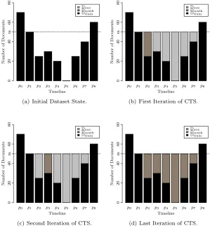
Fig. 1. Example: Effect of Cascading Temporal Smoothing in the Distribution of ClasscOver Time.
the replication of the resulting augmented set of documents ofpj topk. The cascading process works in two stages: (i) a forward cascading, where CTS propagates documents fromlb to p−1, that is, lb→lb+ 1→lb+ 2→ · · · →p−1; and(ii)a backward cascading, where CTS propagates documents from ub to p+ 1, that is, ub → ub −1 → ub−2 → · · · → p+ 1. After that, the neighbors of p have finally been fulfilled with enough documents to be cascaded topand CTS performs the actual oversampling, where the synthetic samples from these neighbors are replicated to the target point in timep. As our goal is to perform the oversampling to pointp, in the two previously described stages of the cascading process—(i)and(ii)—the CTS uses an auxiliary synthetic datasetDauxthat can be
discarded at the end. There are three cases to be considered by the CTS:
(1) Ifpis the first point in time of the dataset (p0), then the CTS performs only a backward cascading
p+ 1→pof (m− |Dc,p|) documents;
(2) Ifpis the last point in time of the dataset (pf), then the CTS performs only a forward cascading p−1→pof (m− |Dc,p|) documents;
(3) Ifpis neither the first nor the last point in time of the dataset, then the CTS performs both a backward and a forward cascading, each with (m−|Dc,p|)
2 documents.
The generated documents are then stored in a set of synthetic documents Dsynth, which will be
merged to the training set at the end of the process.
hypothetical classc. Figure 1(a) shows the initial distribution of classcover time. The CTS algorithm starts withp=p0, and iterates through all points in time till the last one, when p=p8. For each point in timep, CTS evaluates |Dc,p| in order to decide if it shall generate new synthetic documents
for classc. This test is done by line 6 and, for our example, it will be set to true whenp=p2. Let us consider this iteration. The lower and upper bounds, computed by lines 8 and 9, respectively, will be lb=p1andub=p8.5 The algorithm will bypass the lines 10 and 19 and will proceed to the auxiliary synthetic data generation. Sincelb=p2−1 =p1, CTS will not perform the forward cascading (lines 20 to 24), but it will proceed with the backward cascading (lines 25 to 29): p8→p7 →p6→ · · · →p3. After that, the neighbors ofp2 have finally been fulfilled with enough documents to be cascaded to it. The actual oversampling is performed from line 30 to 39, where the synthetic samples from the neighborhood of p2 (p1 and p3) are replicated to the target point in time p2. The distribution of documents of classc after this iteration is illustrated in Figure 1(b). The next iteration sets p=p3, which also does not have enough documents. As before, the algorithm determines the lower and upper bounds, which arelb =p1 andub =p8. The documents are thus cascaded both forwards and backwards, considering the auxiliary datasetDaux: p1 → p2 and p8 → p7 →p6 → · · · → p4. Now,
the neighbors ofp3 are properly fulfilled, and the actual cascading is performed. After this iteration, the augmented dataset looks like Figure 1(c). The algorithm then proceeds to the remaining points in timep4top8, until reaching the final class distribution depicted in Figure 1(d).
Notice that CTS does not aim at balancing the dataset. In fact, CTS promotes a reduction in the observed variations of the target class distribution over time. Thismayreduce the overall class imbal-ance ratio, since the minority classes may not have more thanmdocuments in several points in time. However, this is not true for all cases. For example, consider thatcis the majority class. Also, consider that its documents were created at just a few points in time (that is, in several points in time there are less thanmdocuments assigned to classc). In this case, the CTS algorithm would increase the major-ity class and, consequently, increase the class imbalance ratio. In fact, a perfect balancing is achieved whenm= max(|Dc,p|). However, as we shall see in Section 4, this is may not be the best choice form.
3.2 CTS Analysis
In this section, we consider some properties of the CTS algorithm. More specifically, we shall provide an analysis regarding the behavior of the cascading process performed by CTS and the effect of its pa-rameterm. As we describe below, when cascadingpi→pj, the greater the temporal distance between them, the smaller is the probability of transferring documents frompitopj. This means that CTS will privilege nearby points in time during the cascading process, smoothing out the observed variations in the datasets’ characteristics between these points in time while preventing a random behavior (that is, preventing the transference of documents irrespective to their time points). Moreover, as we shall see, smallermvalues limit CTS capability of smoothing the variations. On the other hand, whenm increases, at the limit, CTS tends to converge into a random oversampling strategy. A good trade-off between CTS smoothing capability and its randomness avoidance can be easily achieved by means of a simple greedy search algorithm, due to this unimodal6 behavior regarding themparameter. So, let
cbe an arbitrary class andmbe CTS threshold. We start our analysis by considering the probability of transferring original data from a source point in timepi to a target point in time pj, denoted by P(pi, pj). Recall that, from the definition of lower and upper bounds, for all points in time p′ ≤lb andp′′≥ub,|Dc,p′| ≥mand|Dc,p′′| ≥m. For these cases, both sets will not be affected by the CTS,
since they are composed by enough documents. Thus, in the following we shall turn our attention to the points in timepi ≥lb and pj ≤ub. Our two base cases to be considered are P(lb, lb+1) = 1
5Ifl
b is undefined, the CTS generates documents for the first point in time p0, setslb =p0 and proceeds as usual.
Ifub is undefined, CTS generates documents for the last point in timep8, setsub=p8and proceeds as usual. Both
situations are handled in lines 10 through 19 of Algorithm 2.
6A functionf(x) is unimodal if it is monotonically increasing forx≤nand monotonically decreasing for x≥n. In
Algorithm 2Cascaded Temporal Smoothing. 1: functionCTS(Dtrain,m)
2: Dsynth← ∅
3: forc∈Cdo
4: forp∈Pdo
5: Dc, p← {d∈Dtrain|d.c=candd.p=p}
6: if |Dc,p|< mthen ⊲Not enough documents inDc,p
7: Daux←Dtrain ⊲Auxiliary data
8: lb←FindLowerBound(c, p, m) 9: ub←FindUpperBound(c, p, m)
10: if lb=N ILthen ⊲Not enough documents betweenp0andp
11: lb←FindUpperBound(c, p,1) ⊲Find nextp′s.t.Dc,p′6=∅
12: Daux←Daux∪GenerateSamples(lb, p0, c,Daux, m)
13: lb←p0 ⊲Lower bound now defined
14: end if
15: if ub=N ILthen ⊲Not enough documents betweenpandpf
16: ub←FindLowerBound(c, p,1) ⊲Find previousp′s.t.D
c,p′6=∅ 17: Daux←Daux∪GenerateSamples(ub, pf, c,Daux, m)
18: ub←pf ⊲Upper bound now defined
19: end if
20: whilelb+ 1< pdo ⊲Forward cascading: from past top
21: n←m− |Dc,lb+1|
22: Daux←Daux∪GenerateSamples(lb, lb+ 1, c,Daux, n)
23: lb←lb+ 1
24: end while
25: whileub−1> pdo ⊲Backward cascading: from future top 26: n←m− |Dc,ub−1|
27: Daux←Daux∪GenerateSamples(ub, ub−1, c,Daux, n)
28: ub←ub−1
29: end while
30: ⊲Actual training set oversampling: 31: n←m− |Dc,p|
32: if p=p0then ⊲Backward Cascading only
33: Dsynth←Dsynth∪GenerateSamples(p+ 1, p, c,Daux, n)
34: else ifp=pf then ⊲Forward Cascading only
35: Dsynth←Dsynth∪GenerateSamples(p−1, p, c,Daux, n)
36: else ⊲Both backward and forward Cascading
37: Dsynth←Dsynth∪GenerateSamples(p+ 1, p, c,Daux,n
2)
38: Dsynth←Dsynth∪GenerateSamples(p−1, p, c,Daux,n
2)
39: end if
40: end if
41: end for
42: end for
43: Dtrain←Dtrain∪Dsynth
44: end function
and P(ub, ub−1) = 1, ∀pj ∈ P. This follows from the definition of lower and upper bounds, where |Dc,lb| ≥ mand|Dc,ub| ≥mand, consequently, all the documents transferred to lb+1 andub−1 come
from lb and ub, respectively. Now, consider the probability P(lb, lb+2), that is, the probability of transferring documents fromlb to lb+2. In this case, after the first cascading lb →lb+1, the point in timelb+1 will be composed by mdocuments such that (m− |Dc,lb+1|) were cascaded fromlb.
7 Thus, the probability of documents fromlb to be cascaded tolb+2 is given by:
P(lb, lb+2) =
m− |Dc,lb+1|
m (1)
The probability of documents from lb to be transferred to lb+3—P(lb, lb+3)—depends on the lb → lb+1,
lb+1→lb+2andlb+1→lb+2cascades, since documents fromlbmust first be cascaded tolb+1, and then tolb+2 and, finally, tolb+3. Thus,P(lb, lb+3) =P(lb, lb+1)·P(lb+1, lb+2)·P(lb+2, lb+3). Substituting the first term by 1 and the second term by Equation 1, we get:
P(lb, lb+3) =
m− |Dc,l b+1|
m ·P(lb+2, lb+3). (2)
7Notice that, by the lower and upper bounds definition, (m− |D
Recall that after the lb+1 → lb+2 cascading, the point in timelb+2 is composed by m documents such that (m− |Dc,l
b+2|) were cascaded fromlb+1. Thus, we are able to substitute the third termP(lb+2, lb+3) of
Equation 2, based on the same rationale employed to derive Equation 1:
P(lb, lb+3) =
m− |Dc,lb+1|
m ·
m− |Dc,lb+2|
m . (3)
It should be straightforward to verify that
P(lb, lb+4) =
m− |Dc,lb+1|
m ·
m− |Dc,lb+2|
m ·
m− |Dc,lb+3|
m .
The above derivations give us the necessary tools to derive a more general formulationP(lb, p),∀p ∈ P, which gives us the probability of transferring data from the lb to a point in time p (through the forward cascading):8
P(lb, p) = Qp
p′=lb+1(m− |
Dc,p′|)
mp−lb−1 . (4)
Analogously to the derivation of P(lb, p) regarding the forward cascading, it is easy to verify that the probabilityP(ub, p) regarding the backward cascading is given by:
P(ub, p) = Qp
p′=lu−1(m− |Dc,p′|)
mub−p−1 . (5)
The last two probabilities give us some clues regarding the behavior of CTS. First, considering the cascading
lb → p (or ub → p), the greater the temporal distance between them, the smaller is the probability of transferring documents from lb (or ub) to p. Consequently, the greater is the probability of transferring synthetic data from nearby points in time. This is a key aspect to guarantee the controlled behavior of the CTS oversampling process. If, despite of prioritizing nearby points in time, CTS associates an uniform probability of propagating documents from any point in time, than it would be equivalent to a random oversampling process. Furthermore, privileging nearby time points also avoids the propagation of very abrupt changes in the dataset characteristics, consequently turning the cascading process smoother. Second, greater
mimplies a higher probability of transferring data from distant point in times top. As we shall elaborate soon, asymptotically, this converges to a simple random oversampling, irrespective of the documents timeliness.
Equations 4 and 5 enable us to determine the probability of transferring documents from the boundary points in time (lband ub) to the target pointpin the actual oversampling step of CTS (lines 30 to 39). As mentioned before, there are three cases to consider: (i) ifp=p0, just the backward cascading occurs, with probability given by Equation 5;(ii)ifp=pf, just the forward cascading occurs, with probability given by Equation 4; finally, ifp6=p0 andp6=pf, then both forward and backward cascading take place (see lines 37 and 38 of Algorithm 2), with probabilities given byP(lb, p) and P(ub, p), respectively. Ifm ≫ |Dc,p| then,
asymptotically,P(lb, p) will converge to
Qp lb+1m
mp−lb−1 = 1, as willP(ub, p). It means that, in all cases, in the limit ofm, all points in time will share similar probabilities of cascading documents to the target pointp, which corresponds to a random oversampling process irrespective to the documents creation time. On the other hand, notice that, ifm≤min(|Dc,p|) than, by construction, CTS will not cascade any document through the timeline. As we shall see, this unimodal behavior can be exploited to efficiently calibrate the CTS. Sincecis arbitrary, then the above discussion holds for all classes of the dataset.
4. EXPERIMENTAL EVALUATION
In this section, we describe our experimental setup, namely, the explored datasets and algorithms, as well as report and analyze our achieved results.
8We removed the probability associated to the cascadingl
4.1 Testbed
The two reference datasets considered in our study consist of sets of large textual documents, each one assigned to a single class (a single label problem). The considered datasets9 are:
(1) ACM-DL:This dataset [Couto et al. 2006] is a subset of the ACM Digital Library with 24,897 docu-ments containing articles related to Computer Science created between 1980 and 2002. We considered the first level of the taxonomy in the ACM-DL Computing Classification System (CCS), including 11 classes, which remained the same throughout the period of analysis.
(2) MEDLINE:This dataset [Mour˜ao et al. 2008] is a subset of the MedLine dataset, with 861,454 docu-ments classified into 7 distinct classes related to Medicine, and created between the years of 1970 and 1985.
Recall that each documentdiof these datasets are represented as triplesdi=hxi, ci, piisuch thatxidenotes the vector representation ofdi,ci represents its assigned class andpi represents its creation time. Since the explored datasets refer to scientific articles, a natural time granularity forpiis the year, since scientific confer-ences are usually annual. Thus,pi denotes the yeardi was created. In order to evaluate the CTS algorithm, we considered four classification tasks, as detailed below:
Traditional. This classification task is characterized by learning a classification model based on the original training setDtrainand then using it to classifyDtest. We adopted the Na¨ıve Bayes, since its temporally-aware
version was the top performer in the explored datasets as shown in [Salles et al. 2010]. Such classifier is a probabilistic learning method that aims at inferring a model for each class by assigning to a test documentd′
the class associated with the most probable model that would have generated it (i.e., the class with maximum a posteriori probability). Here, we adopt the Multinomial Na¨ıve Bayes approach, since it is widely used for probabilistic text classification. The posterior class probabilitiesP(d′|c) are defined as:
P(d′|c) =η×P(c)×Y
t∈d′
P(t|c),
whereηdenotes a normalizing factor,P(c) is the class prior probability andP(t|c) denotes the conditional probability of observingthaving already observedc.As said, such classifier assigns to a test example d′ the
classcwith the highest a posteriori probabilityP(d′|c). BothP(c) andP(t|c) are estimated from the observed frequency of occurrences of documents and terms in the classes, irrespective of the documents timeliness. Furthermore, these probabilities are approximated by a maximum likelihood method, depending solely on the training set. We expect this to be the fastest classification scenario (low runtime for both the training and test-ing phases), but the one most influenced by the temporal effects, as there are no explicit treatments for them. Temporally-Aware. This classification task is characterized by applying a Temporally-Aware classifier [Salles et al. 2010], learned from the original training setDtrain and used to classifyDtest. For this purpose, we chose the Temporally-Aware Na¨ıve Bayes classifier, with the temporal weighting function (see Section 2) applied in documents. This was the best performing temporally-aware classifier for the two adopted datasets, as reported in [Salles et al. 2010]. In this strategy, atemporal weighting function(TWF) is used to control the influence of training documents used for probability estimation (namely the relative frequencies of occurrences of docu-ments and terms for each class, as time goes by) according to the temporal distance between training and test data. The TWF reflects the observed evolution of the term-class relationships over time, and its expression is determined by means of a series of statistical tests. Then, a curve fitting procedure is employed to determine its parameters. A detailed description about the TWF can be found in [Salles et al. 2010]. The Temporally-Aware Na¨ıve Bayes classifier learns the probability of assigning a test documentd′to classcas follows:
P(d′|c) =η·
P
p(Ncp·T W F(δ)) P
p(Np·T W F(δ))
·Y
t∈d′ P
p(ftcp·T W F(δ)) P
p P t′∈V
(ft′cp·T W F(δ))
,
whereDdenotes the training set,ηdenotes a normalizing factor,Ncpis the number of training documents ofDassigned to classcand created at the time pointp,Npis the number of training documents created at the time pointp,ftcpstands for the frequency of occurrence of termtin training documents of classcthat were
created on time pointp, TWF denotes the temporal weighting function and, finally, δ denotes the temporal distance betweenp and the creation time of d′ (a.k.a., the reference point in timep
r). Notice that, in this case, both the a priori class probabilities and the term conditionals depend on the temporal distance between training documents and the test. This obligates the classifier to postpone the estimation of these probabilities until it receives the test document, thus characterizing a lazy classifier. We expect this scenario to have the higher test runtime, since it must iterate overp∈P, considering its temporal distance to the reference point
pr, in order to properly estimate both the class a priori and term conditional probabilities. We consider it as our upper bound in terms of handling the temporal effects.
CTS. This classification task involves learning a probabilistic model for the traditional Na¨ıve Bayes algo-rithm, based on the augmented training setDtrain∪Dsynth generated by CTS. That is, we first apply the CTS algorithm to the original training set, considering a thresholdm (which ultimately determines|Dsynth|), and
then use the new augmented training set to learn a traditional Na¨ıve Bayes classifier.
Random. This classification task serves the purpose of isolating the improvements made by the CTS al-gorithm from the random oversampling effect, and provide evidence about the analysis done in Section 3.2 regarding the influence ofmin CTS. In this case, the training setDtrainis randomly oversampled with exactly
the same number os documents generated by the CTS approach. In this case, we do not perform cascading (that is, the random oversampling is performed irrespective to the timeline). The augmented training set have the same number of documents as the training set of “CTS” task.
4.2 Results
Recall that our goal is twofold: (i) to provide an effective document classification, robust to the temporal dynamics;(ii)which, at the same time, scales with the test set size. Hence, our experimental evaluation will be held considering two dimensions: classification effectiveness and scalability. As we shall see, the CTS was able to significantly improve classification effectiveness, while being scalable enough to handle large volumes of data. Furthermore, for all the described tasks, the test data is presented to the classifier without any temporal ordering, during the test phase. The following experiments were performed in a IntelR
CoreTMi7 CPU (2.93GHz) with 8GBof RAM. We start by analyzing the classification effectiveness.
4.2.1 Effectiveness Analysis. In order to evaluate the impact that CTS has in the classification effective-ness, we compare the four tasks previously described applied to both adopted datasets (ACM-DL and MED-LINE). For comparison we use a standard information retrieval measure commonly adopted for multi-class clas-sification problems, namely, the macro averaged F1 (MacroF1) measure. The MacroF1 is given averaging the
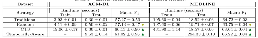
F1measure (i.e., the harmonic mean of precision and recall) obtained for each individual class. All experiments were performed using a 10-fold cross-validation [Kohavi 1995] in order to assess the statistical validity of the obtained results and their 99% confidence intervals for the mean. At each iteration of the cross validation pro-cess, another 3-fold cross-validation over thetraining set was used to calibrate themparameter. We searched for values ofmin the interval from 10 to 1,000 (with steps of 10) and from 100 to 10,000 (with steps of 100), for the ACM-DL and MEDLINE datasets, respectively. These intervals were selected according to the dataset size. We also explored the discussed unimodal behavior regarding them value (see Section 3.2) by greedily stopping the search when observing a decrease in MacroF1. Once the best value was determined, it was fixed and used to finally augment the training set. The augmented training set was then used to learn a classification model to classify the test set. Themvalue chosen was also used by the “Random” task in order to enable us to isolate the cascading effect, as we shall see soon. The results obtained for the ACM-DL and MEDLINE datasets are reported in Table I. In that table, we reported the time spent by the train and test phases, along with the obtained MacroF1, for each described task. The symbol following the MacroF1 values refers to the statistical significance test, assessed by a paired two-sided t-test with 99% confidence level. Ndenotes a statistically
sig-nificant improvement over the “Traditional” task and•denotes a statistical tie. The training phase runtime of the “CTS” task covers the time spent both to tunem(through cross-validation) and to learn a classifier. Finally, as the temporally-aware classifier is inherently lazy, we just report the runtime associated with the test phase.
Table I. Effectiveness Analisys: Obtained Results.
Dataset ACM-DL MEDLINE
Strategy Runtime (seconds) Macro-F1 Runtime (seconds) Macro-F1
Train Test Train Test
Traditional 3.93±0.01 0.30±0.01 57.27±0.50 195.60±0.04 18.52±0.06 64.72±0.03 Random 4.11±0.09 0.50±0.02 57.13±0.47• 197.60±0.06 19.71±0.07 63.75±0.04•
CTS 19.06±0.17 0.30±0.01 60.13±0.90N 431.90±1.14 18.57±0.06 68.04±0.04N Temporally-Aware – 9.53±0.14 61.02±0.98N – 294.33±0.10 66.22±0.04N
cascading ? In other words, we must isolate the obtained improvements and determine if it was a result of considering the documents’ timeliness when propagating them, or if the same improvements should be achieved by randomly oversampling the dataset. This question is answered by considering the “Random” classification task. As it can be observed, CTS performs better than a simple random oversampling strategy (with a gain of 5.25% over the “Random” task), while the “Random” task was no better than the traditional classifier. Thus, the improvements achieved by CTS can in fact be explained by the smoothing of the temporal effects. However, this improvement comes with an extra cost: one needs to properly calibrate the CTS parameter and to execute the CTS, which may impose an additional runtime to the training phase. In fact, as it can be ob-served from Table I, the training phase runtime of “CTS” is greater than the “Traditional” training time. Such runtime is also greater than the time spent by the temporally-aware classifier. However, we think the benefits obtained by the CTS are worth, for two reasons. First, such pre-process step is executed only once, before learning and deploying the classification system. Second, unlike the CTS approach, the lazy temporally-aware classifier has a critical scalability issue, as we shall see in Section 4.2.2.
Turning our attention to the MEDLINE dataset, in Table I we can observe that the temporally-aware clas-sifier outperformed the traditional clasclas-sifier in terms of MacroF1. Such result is also in conformity with those reported in [Salles et al. 2010]. However, the key aspect here is the behavior of CTS. In fact, CTS improved the classification effectiveness in terms of MacroF1, with a gain of 5.13% over the “Traditional” task and a gain of 6.73% over the “Random” task. Furthermore, it was statistically superior to the temporally-aware classifier, with a marginal gain of 2.75% in MacroF1. Considering that the CTS performed better than the “Random” task and was competitive to the temporally-aware classifier, it means that CTS was indeed able to tackle the temporal effects. Again, this improvement comes with a cost of an additional step at training phase. But, as we have already stated, such additional step is performed only once, before the classifier deployment. Further-more, as we will discuss next, unlike CTS, the temporally-aware classifier does not scale well with the test set.
Finally, let us consider the behavior of CTS with regards to them parameter. In order to have a better understanding about how the m values influence the classification effectiveness (in terms of the discussed unimodal behavior of CTS w.r.t. m), we explicitly varied such parameter and evaluate the obtained MacroF1, for both the “CTS” and the “Random” task. Such evaluation is reported in Figure 2 and serves the unique purpose of corroborating the probabilistic analysis done in Section 3.2. As we can see for both datasets, for smaller values of mthe capability of CTS to smooth the temporal variations is smaller, as reflected by the lower MacroF1. On the other hand, asmincreases the MacroF1 also increases. But such improvement occurs up to a certain level at which the CTS performance converges to the performance of the “Random” task. This is in consonance with the probabilistic analysis presented in Section 3.2. The proper calibration ofm
aims at producing a good compromise between the smoothing capability of CTS while preventing the CTS to degenerate into a case in which it performs purely randomly (irrespective to the timeliness). This observed unimodal behavior of the CTS with regard to the values ofmmakes the choice of this parameter easily tunable by some greedy searching algorithm. Such property is useful for practical application.
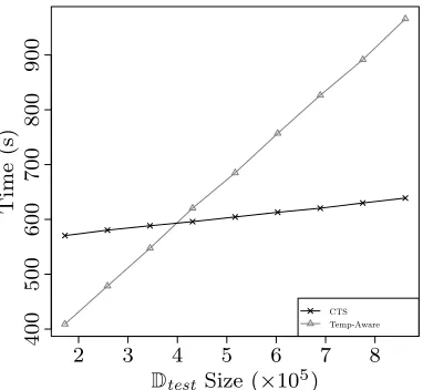
4.2.2 Scalability Analysis. Recall that, besides maintaining the classification task robust to the tempo-ral effects, our main motivation is to reduce the test phase runtime. More specifically, we aim at providing a strategy to tackle the temporal effects in a scalable way, which is able to classify large sets of data in a reasonable amount of time. As we have seen, CTS indeed maintains such temporal robustness, achieving statistically equivalent (or even superior) results to those obtained by the temporally-aware algorithm. Now, we turn our attention to runtime and scalability issues.
(a) ACM-DL Dataset. (b) MEDLINE Dataset.
Fig. 2. An Analysis Regarding the Effect ofmin the CTS Algorithm.
generated a new test setD′
test such that|D′test|=i× |Dtest|. This was accomplished by concatenating Dtest
with itselfitimes. Then, for each|D′test|we measured the time spent to classify this test set by both CTS and temporally-aware settings. More specifically, for the CTS we measured the time spent to calibratemthrough cross-validation over the training set, together with the time spent to train and test. For the temporally-aware approach, we measured the time spent to classifyD′
test (recall that this is a lazy approach). This experiment
was replicated 10 times by means of a 10-fold cross-validation, and the averaged measurements are reported in Figure 3.
As we can see in Figure 3, as the test set size increases, the runtime of the temporally-aware approach increases much faster than the CTS approach. This is explained by the lazy nature of the former: for each test document the training set must be revisited in order to learn the classification rules according to the observed temporal distance between training and test documents. Thus, as|D′
test|increases the cost of this approach
2 3 4 5 6 7 8
4
0
0
5
0
0
6
0
0
7
0
0
8
0
0
9
0
0
Dtest Size (×105)
T
im
e
(s
)
CTS Temp-Aware
may become infeasible for very large collections such as the Web or very large digital libraries.10 On the other hand, we observe that the time spent by the CTS approach increases in a much smaller rate, meaning that the throughput of the classifier employing the CTS (in terms of classified documents per time unit) is superior to the throughput of the temporally-aware classifier. This highlights the practical applicability of CTS when classifying large amounts of data, without being compromised by the temporal effects observed in training data. Finally, the CTS and its possible derived approaches (such as CTS with SMOTE replication) open opportunities for future developments using new classifiers whose lazy versions would be infeasible to deal with the temporal effects in large datasets (e.g., SVM).
5. CONCLUSIONS AND FUTURE WORK
This work proposed a data engineering strategy aimed at preventing a classifier to be negatively impacted by the observed temporal effects in textual datasets. Such strategy, called Cascaded Temporal Smoothing, is char-acterized by handling the temporal effects in an entirely off-line setting by means of a controlled cascading of documents through the timeline in order to smooth out these effects in the training data. Unlike the previously proposed temporally-aware classifiers, our strategy does not incur in any overhead at the test phase, offering good scalability when tackling such issue, while not compromising the classification effectiveness. Thus, we can summarize the CTS advantages over the temporally-aware classifiers previously proposed, as being:
(1) the use of CTS does not involve any modifications on existing classification algorithms, ultimately being independent of classifier and ensuring its applicability in already consolidated automatic classification techniques (some of which were previously very difficult to extend by the fact that our temporally-aware solutions were inherently lazy);
(2) since CTS moves all the overhead of tackling the temporal effects to an off-line setting, its use maintains the classification throughput of the traditional classifiers while increasing classification effectiveness.
Clearly, there is room for further improvements in, at least, three directions. First, the synthetic data gen-erator can be made much more sophisticated. Besides simple replication, as adopted by CTS, we can use other strategies, as SMOTE [Chawla et al. 2002] or the probabilistic generation strategy discussed in [Chen et al. 2011; Bermejo et al. 2011].The use of SMOTE when generating new samples for CTS may be advantageous since it defines less specific class boundaries with the introduction of new informative instances (which can not be achieved by simple replication). A probabilistic based sample generation can be even more advantageous since, besides generating informative instances, it is also able to reduce inter-class overlapping, which is a well known challenge in automatic classification. Second, we may significantly reduce the computational cost of CTS, eliminating the needs of maintaining the auxiliary dataDaux, by directly determining the probability of sampling documents according to their creation time and the dataset temporal dynamics (e.g., considering the stability level of documents [Salles 2011] to determine the documents to be propagated through the timeline). Third, based on the probabilistic analysis of CTS, we plan to extend CTS to automatically adjust the number of documents to be transferred from the lower and upper bounds lb and ub to the target point in timep according to the temporal distance between them, in a way that the user will not need to tune the parameter
manymore. Moreover, we will apply the CTS in scenarios where the previously proposed temporally-aware solutions are infeasible due to the lazy requirement (e.g., SVM). Finally, we plan to provide a quantitative analysis regarding the temporal effects, as done in [Salles 2011], before and after the application of CTS in the dataset, in order to provide a better understanding regarding the behavior of CTS with relation to these effects.
REFERENCES
Bermejo, P.,G´amez, J. A.,and Puerta, J. M. Improving the performance of Naive Bayes multinomial in e-mail foldering by introducing distribution-based balance of datasets.Expert Systems with Applications38 (3): 2072–2080, 2011.
Chawla, N.,Bowyer, K.,Hall, L.,and Kegelmeyer, W. SMOTE: Synthetic Minority Over-sampling Technique. Journal of Artificial Intelligence Researchvol. 16, pp. 321–357, 2002.
10Notice also that the number of classes in the experimented tasks is small (i.e., 11 classes in ACM-DL and 7 classes in
Chen, E.,Lin, Y.,Xiong, H.,Luo, Q.,and Ma, H. Exploiting Probabilistic Topic Models to Improve Text Catego-rization Under Class Imbalance.Information Processing & Management 47 (2): 202–214, 2011.
Chiang, J.-H. and Chen, Y.-C.An Intelligent News Recommender Agent for Filtering and Categorizing Large Volumes of Text Corpus.International Journal of Intelligent Systems19 (3): 201–216, 2004.
Cohen, W. W. and Singer, Y. Context-Sensitive Learning Methods for Text Categorization. ACM Transactions on Information Systems17 (2): 141–173, 1999.
Couto, T.,Cristo, M.,Gon¸calves, M. A.,Calado, P.,Ziviani, N.,Moura, E.,and Ribeiro-Neto, B.A Compar-ative Study of Citations and Links in Document Classification. InProceedings of the ACM IEEE Joint Conference on Digital Libraries. Chapel Hill, USA, pp. 75–84, 2006.
Crammer, K.,Dekel, O.,Keshet, J.,Shalev-shwartz, S.,and Singer, Y. Online Passive-Aggressive Algorithms. Journal of Machine Learning Researchvol. 7, pp. 551–585, 2006.
Fdez-Riverola, F.,Iglesias, E.,D´ıaz, F.,M´endez, J.,and Corchado, J. Applying Lazy Learning Algorithms to Tackle Concept Drift in Spam Filtering. Expert Systems with Applications33 (1): 36–48, 2007.
Forman, G.Tackling Concept Drift by Temporal Inductive Transfer. InProceedings of the International ACM SIGIR Conference on Research & Development of Information Retrieval. Washington, USA, pp. 252–259, 2006.
Klinkenberg, R.Learning drifting concepts: Example selection vs. example weighting.Intelligent Data Analysis8 (3): 281–300, 2004.
Klinkenberg, R. and Joachims, T. Detecting Concept Drift with Support Vector Machines. In Proceedings of the International Conference on Machine Learning. Stanford, USA, pp. 487–494, 2000.
Kohavi, R.A Study of Cross-Validation and Bootstrap for Accuracy Estimation and Model Selection. InProceedings of the International Joint Conference on Artificial Intelligence. Qu´ebec, Canada, pp. 1137–1143, 1995.
Koren, Y. Collaborative Filtering with Temporal Dynamics.Communications of the ACM vol. 53, pp. 89–97, 2010.
Mour˜ao, F.,Rocha, L.,Ara´ujo, R.,Couto, T.,Gon¸calves, M.,and Meira Jr., W. Understanding Temporal Aspects in Document Classification. InProceedings of the International Conference on Web Search and Web Data Mining. Palo Alto, USA, pp. 159–170, 2008.
Pan, S. J. and Yang, Q. A Survey on Transfer Learning. IEEE Transactions on Knowledge and Data Engineer-ing22 (10): 1345–1359, 2010.
Rajan, S.,Yankov, D.,Gaffney, S. J.,and Ratnaparkhi, A. A Large-Scale Active Learning System for Topical Categorization on the Web. InProceedings of the International Conference on World Wide Web. Raleigh, USA, pp. 791–800, 2010.
Rocha, L.,Mour˜ao, F.,Pereira, A.,Gon¸calves, M. A.,and Meira Jr., W.Exploiting Temporal Contexts in Text Classification. InProceedings of the International Conference on Information and Knowledge Engineering. Napa Valley, USA, pp. 243–252, 2008.
Salles, T.Automatic Document Classification Temporally Robust. M.Sc. Thesis, Federal University of Minas Gerais, Belo Horizonte, Brazil, 2011.
Salles, T.,Rocha, L.,Pappa, G. L.,Mour˜ao, F.,Gon¸calves, M. A.,and Jr., W. M.Temporally-Aware Algorithms for Document Classification. InProceedings of the International ACM SIGIR Conference on Research & Development of Information Retrieval. ACM Press, Genebra, Switzerland, pp. 307–314, 2010.
Tsymbal, A.The Problem of Concept Drift: Definitions and Related Work. Technical report, Department of Computer Science, Trinity College, Dublin, Ireland, 2004.
ˇ
Zliobait ˙e, I. Combining time and space similarity for small size learning under concept drift. InProceedings of the International Symposium on Foundations of Intelligent Systems. Prague, Czech Republic, pp. 412–421, 2009.
Wang, H.,Yu, P. S.,and Han, J. Mining Concept-Drifting Data Streams. InData Mining and Knowledge Discovery Handbook, O. Maimon and L. Rokach (Eds.). Springer, pp. 789–802, 2010.
Widmer, G. and Kubat, M.Learning in the Presence of Concept Drift and Hidden Contexts.Machine Learning23 (1): 69–101, 1996.