Parallel Computing of Particle Filtering Algorithms for Target Tracking Applications

(1)

University of New Orleans University of New Orleans

ScholarWorks@UNO

University of New Orleans Theses and

Dissertations Dissertations and Theses

Fall 12-18-2014

Parallel Computing of Particle Filtering Algorithms for Target

Tracking Applications

Jiande Wu

University of New Orleans, [email protected]

Follow this and additional works at: https://scholarworks.uno.edu/td

Part of the Electrical and Computer Engineering Commons

Recommended Citation Recommended Citation

Wu, Jiande, "Parallel Computing of Particle Filtering Algorithms for Target Tracking Applications" (2014). University of New Orleans Theses and Dissertations. 1953.

https://scholarworks.uno.edu/td/1953

This Dissertation-Restricted is protected by copyright and/or related rights. It has been brought to you by ScholarWorks@UNO with permission from the rights-holder(s). You are free to use this Dissertation-Restricted in any way that is permitted by the copyright and related rights legislation that applies to your use. For other uses you need to obtain permission from the rights-holder(s) directly, unless additional rights are indicated by a Creative Commons license in the record and/or on the work itself.

This Dissertation-Restricted has been accepted for inclusion in University of New Orleans Theses and Dissertations by an authorized administrator of ScholarWorks@UNO. For more information, please contact

(2)

Parallel Computing of Particle Filtering Algorithms for Target Tracking Applications

A Dissertation

Submitted to the Graduate Faculty of the University of New Orleans

in partial fulllment of the requirements for the degree of

Doctor of Philosophy in

Engineering and Applied Science

by Jiande Wu

B.S. North China Electric Power University, 1998 M.S. North China Electric Power University, 2005

(3)

c

(4)

Acknowledgements

I would like to express my sincere thanks to lots of people without whom this dissertation would not have been possible.

To my advisor, Dr. Vesselin Jilkov, who is always a source of knowledge and inspiration for me.

To Dr. X. Rong Li and Dr. Huimin Chen who also provide me invaluable and insightful thinking and guidance during my research.

To my committee members, Dr. Shengru Tu and Dr. George Ioup, for their great effort and help on my dissertation.

To my colleagues and friends, Dr. Zhansheng Duan, Dr. Yu Liu, Dr. Xiaomeng Bian, Dr. Meiqin Liu, Dr. Ji Zhang, Dr. Yongxin Gao, Ms. Jing Hou, Mr. Haozhan Meng and Mr. Gang Liu, without whom, my life during the PhD study in UNO would become much harder. Without these people, I can hardly make this journey. I dedicate this dissertation to them. Furthermore, I want to thank all the members and staff of the Department of Electrical Engineering at the University of New Orleans for their service and support.

Last but not least at all, to my parents, my wife, my sister and my children, who con-tinuously support and encourage me throughout my study and research.

(5)

Particle filtering has been a very popular method to solve nonlinear/non-Gaussian state estimation problems for more than twenty years. Particle filters (PFs) have found lots of applications in areas that include nonlinear filtering of noisy signals and data, especially in target tracking. However, implementation of high dimensional PFs in real-time for large-scale problems is a very challenging computational task.

Parallel & distributed (P&D) computing is a promising way to deal with the computa-tional challenges of PF methods. The main goal of this dissertation is to develop, implement and evaluate computationally efficient PF algorithms for target tracking, and thereby bring them closer to practical applications. To reach this goal, a number of parallel PF algo-rithms is designed and implemented using different parallel hardware architectures such as Computer Cluster, Graphics Processing Unit (GPU), and Field-Programmable Gate Array (FPGA). Proposed is an improved PF implementation for computer cluster - the Particle Transfer Algorithm (PTA), which takes advantage of the cluster architecture and outper-forms significantly existing algorithms. Also, a novel GPU PF algorithm implementation is designed which is highly efficient for GPU architectures. The proposed algorithm imple-mentations on different parallel computing environments are applied and tested for target tracking problems, such as space object tracking, ground multitarget tracking using image sensor, UAV-multisensor tracking. Comprehensive performance evaluation and comparison of the algorithms for both tracking and computational capabilities is performed. It is demon-strated by the obtained simulation results that the proposed implementations help greatly overcome the computational issues of particle filtering for realistic practical problems.

(8)

List of Figures

3.1 Target Trajectory Estimation; Single MC Run; 500 Iterations. . . 28

3.2 Tracking Performance & Execution Time; 64 Processors; 100 MC Runs. . . . 30

3.3 Execution Time, Speedup & Efficiency; 150K Particles. . . 33

3.4 Scenarios with 20 Targets (top) and 50 Targets (bottom). . . 40

3.5 Position TARMSE; 64 Processors; 50 Targets; 100 MC Runs. . . 41

3.6 Average Execution Time; 64 Processors; 50 Targets; 100 MC Runs. . . 42

3.7 Execution Time (top) in Log-scale, Speedup (middle), Efficiency (bottom); 50 Targets; 100K Particles. . . 46

3.8 Execution Time; 64 Processors; 100K Particles. . . 47

3.9 Unbalanced Stratified Resampling . . . 48

3.10 Particle Transfer Algorithm (PTA) . . . 48

3.11 Position TARMSE; 64 Processors; 50 Targets; 100 MC Runs. . . 49

3.12 Execution Time; 64 Processors. . . 50

3.13 Execution Time (top) in Log-scale, Speedup (middle), Efficiency (bottom); 50 Targets; 100K Particles. . . 51

4.1 Nvidia GPU Architecture . . . 55

4.2 Scenario with 20 Targets. . . 62

4.3 Relative Times Spent in the Different Steps Using GPU-DR. . . 63

4.4 Computation Times of CR & DR. . . 64

4.5 Position TARMSE; 3 Targets; 100 MC Runs. . . 64

4.6 Average Execution Time; 3 Targets; 100 MC Runs. . . 65

4.7 Position TARMSE; 20 Targets; 100 MC Runs. . . 65

4.8 Average Execution Time; 20 Targets; 100 MC Runs. . . 66

4.9 Dimension-Free Errors . . . 70

4.10 Time-Averaged Dimension-Free Error (left) & Running Time (right) . . . 72

4.11 One-Step Running Time . . . 73

4.12 Speedup of PF & PFF . . . 74

4.13 Speedup of PF vs. PFF . . . 75

4.14 Parallel Cumulative Sum . . . 76

4.15 Illustration of the Improved GPU PF . . . 77

4.16 Computation Times of CR & DR . . . 79

4.17 Relative Times Spent in the Different Steps Using GPU-DR . . . 79

4.18 Scenario of UAV-Multisensor Tracking . . . 80

(9)

4.20 Time Average RMSE vs. Running Time . . . 84

5.1 FPGA Architecture with four PEs . . . 87

5.2 FPGA TARMSE . . . 93

(10)

List of Tables

2.1 Generic SIS/R PF Algorithm [2] . . . 8

2.2 Gaussian Exact Particle Flow Algorithm [47] . . . 14

3.1 Execution Times . . . 31

3.2 Computational Performances; 100K Particles . . . 32

3.3 Execution Time(s); 50 Targets . . . 43

3.4 Computational Performances; 100K Particles, 50 Targets . . . 44

4.1 Parallel PF Algorithm for GPU . . . 58

4.2 Parallel PFF Algorithm for GPU . . . 60

4.3 Hardware Used for the Simulation . . . 63

4.4 Hardware Used for Design & Simulation . . . 67

4.5 GPU Blocks’ Specification . . . 67

4.6 Running Time (s) . . . 75

4.7 Improved Parallel PF Algorithm for GPU . . . 78

(11)

Chapter 1 Introduction

Particle filtering (PF) was originally proposed in [35]. Due to its generality and simplicity, PF has become a topic of constantly growing interest, development and numerous target tracking applications, e.g. [75]. Particle filters are a group of posterior density estimation algorithms that estimate the posterior density of the state-space by directly implementing the Bayesian filtering approach. This is a recursive algorithm. It consists of two parts: prediction and update. If the variables are linear and normally distributed the Bayesian filter becomes equal to the Kalman filter [78]. The Bayesian filter is also used in computer science for calculating the probabilities of multiple beliefs.

Formally, let_{xk}_k₌₁_,₂_{, ...} be a vector valued discrete-time Markov process with state

tran-sition probability density function(PDF) p(xk|xk−1), and let {zk}_k₌₁_,₂_{, ...} be another process,

stochastically related to _{xk}_k₌₁_,₂_{, ...} through the likelihood p(zk|xk). xk and zk are the state

and the measurement, respectively, andp(xk|xk−1) andp(zk|xk) represent the state and

(12)

p(xk|zk) via the following prediction – update scheme [58]:

p(xk−1|zk−1)−→p(xk|zk−1)−→p(xk|zk) (1.1)

given the initial state PDF p(x0) and a sequence of measurements zk ={z1, ..., zk}.

PF methods use a set of particles to represent the posterior density. These filtering methods make no restrictive assumption about the dynamics of the state-space or the density function. PF methods provide a well-established methodology for generating samples from the required distribution. The state-space model can be non-linear and the initial state and noise distributions can take any form.

However, PFs are not practical yet, due to their excessive computational and memory cost. A natural approach to overcome this prohibitive limitation is to employ parallel & distributed(P&D) computing. Development of P&D algorithms and architectures that utilize the spatial and temporal concurrency of PF computations is a possibility to make the PF-based multiple target tracking, and particle filtering in general, practical. This possibility has not been much studied so far, even though useful work has been done in this direction, e.g., [6, 84, 9, 8, 10, 56]. The most critical and computationally expensive in every implementation of particle filtering is the resampling. Resampling is in effect discarding of samples that have small probability and concentrating on samples that are more probable. In parallel implementations, resampling becomes a bottleneck due to its inherently sequential nature.

(13)

This dissertation addresses the computational challenges of PF and PFF. The main goal is to propose, develop and implement computationally efficient algorithms for particle and particle flow filters for target tracking, and thereby bring them closer to practical application. Parallel & distributed [3] computing is a natural way to overcome this challenge. Thus, to reach this goal, a number of parallel particle and particle flow filter algorithms are designed and implemented using different parallel hardware architectures, such as computer cluster, graphics processing unit (GPU), and field-programmable gate array (FPGA).

This dissertation is organized in six chapters. In these chapters, the motivation, contri-butions and results are described. Throughout the dissertation, performances of particle and particle flow filters are estimated and filter implementation prototypes are built for target tracking applications.

Chapter 1 introduces the background, motivation and goal of this research work.

Chapter 2 briefly surveys the related work, including nonlinear density estimation, and characterization of parallel algorithms and parallel architectures.

Chapter 3 proposes an improved parallel PF algorithm implementation that is more suit-able for computer cluster architecture. Cluster implementation of target tracking problems for space object tracking, and for ground multitarget tracking using image sensor is con-ducted and the performance evaluated. Our algorithm has significant advantage in terms of computational performances as compared to other parallel PF algorithms. On the other hand, its tracking performance degradation is not that significant.

(14)

in both estimation accuracy and computational efficiency. The chapter also develops a GPU implementation of the exact PFF and shows that it has a superior computational performance as compared to the PF implementations.

Chapter 5 proposes a particle flow filter implementation on FPGA. A simple non-linear system, which is typically studied in the context of stochastic system is used as a simulation model. This chapter also analyzes PF & PFF algorithms performance in FPGA architecture in terms of computational complexity and potential throughput.

(15)

Chapter 2 Background of Related Work

2.1 Particle Filtering

2.1.1 Models

Let_{xk}_k₌₁_,₂_{, ...} be a vector valued discrete-time Markov process with state transition

prob-ability density function (PDF) p(xk|xk−1) as given by (2.1a), and let{zk}_k₌₁_,₂_{, ...} be another

process, stochastically related to _{xk}_k₌₁_,₂_{, ...} through the likelihood p(zk|xk) as given by

(2.1b). xk and zk are the state and the measurement, respectively, and p(xk|xk−1) and

p(zk|xk) are the state and measurement models in terms of probability distributions, i.e.,

xk∼p(xx|xk−1) (2.1a)

zk∼p(zk|xk) (2.1b)

(16)

Most often the state and measurement models are given in state-space representation

xk+1 =f(xk, wk) (2.2a) zk =h(xk, vk) (2.2b)

where f and h are the state and measurement function, and wk and vk denote the process

and measurement noises, respectively. The relationship between (2.1) and (2.2) can be find in [58].

2.1.2 Bayesian Recursive Filter

The exact Bayesian recursive filter (BRF) provides the posterior densityp(xk|zk), givenp(x0)

and measurements zk ₌_{_z

1, ..., zk}through the following recursion [58]:

p(xk|xk−1) zk →p(zk|xk)

↓ ↓

p(xk−1|zk−1) −→ p(xk|zk−1) −→ p(xk|zk)

(Prediction) (Update)

The prediction is given by

p(xk|zk−1) =

Z

Rnx

p(xk|xk−1)p(xk−1|zk−1)dxk−1. (2.3)

The update is given by

p(xk|zk) =

p(zk|xk)p(xk|zk−1) p(zk|zk−1)

, (2.4)

where p(zk|zk−1) =

R

Rnxp(zk|xk)p(xk|z

k−1₎_dx

k is the normalization constant.

(17)

ˆ

xMMS

k and its covariancePkMMS|k are computed:

ˆ

xMMS

k|k =

Z

xkp(xk|zk)dxk (2.5a) PMMS

k|k =

Z

(xk−xˆMMSk )(xk−xˆMMSk ) T_p₍_x

k|zk)dxk. (2.5b)

2.1.3 Basic Particle Filter (PF)

PF methods use a set of particles to represent the posterior density. These filtering methods use an assumption about the dynamics of the state-space or the density function models (2.2) or (2.1), respectively. PF methods provide a well-established methodology for generating samples from the required posterior distribution. The state-space model can be non-linear and the initial state and noise distributions can take any form.

Generic SIS/R PF Algorithm

In particle filtering the probability density functions (PDFs) are represented approximately through a set of random samples (particles) and the BRF (1.1) is performed directly on these samples. Most PFs are based on two principal components [2]: sequential importance sampling (SIS) and resampling (R) as given in Table 2.1.

The importance distribution π(_·) must contain the support of the posterior and is to be designed. One possibility is to choose π = p( xk|xik−1) [35] which is often referred to as

(18)

Table 2.1: Generic SIS/R PF Algorithm [2]

• Importance Sampling (IS) – For i= 1, . . . ,N¯

Draw a sample (particle): x¯i

k ∼π xk|xik−1, zk

Evaluate importance weights ¯

wi k =w

i k−1

p(zk|xik)p(x i k|x

i k−1)

π(xi_k|xi_k−1,zk)

– For i= 1, . . . ,N¯

Normalize importance weights: wi k =

¯

wi k PN¯

j=1w¯

j k • Resampling (R)

– Effective sample size estimation: ˆNef f = PN 1 j=1(w

j k)

2

– If ˆNef f < Nth

Sample from

¯

xj_k, wj_k N_j₌₁ to obtain a new sample set nxi

k = ¯x ji

k, w i k= 1 N oN i=1

2.1.4 Resampling Algorithms Review

The resampling step modifies the weighted approximate density to an unweighted density by deleting particles having low importance weights and by copying particles having high importance weights. In the particle filter literature [5, 34, 37, 40, 41, 54, 57, 64, 69, 70, 81, 87] four basic resampling algorithms can be identified [29], as given next.

Multinomial resampling

This approach to resampling is based on an idea of the bootstrap method [31]. It is known as multinomial resampling since the duplication countsN1, . . . , Nmare by definition distributed

according to the multinomial distribution Mult(n;w1, . . . , wm).

Sampling each x(k) _{independently from the distribution associated with} _{_x_˜(i)_,_w_˜(i)_}N i=1

(19)

M(_·;N,_{w˜(i)_}N

i=1), which has the probability mass function:

M(n1, . . . , nN;N,{w˜(i)}Ni=1) =

    

N!

QN

i=1ni!

QN

i=1( ˜w(i))ni if

PN

i=1ni =N,

0 otherwise.

(2.6)

Stratified Resampling

Stratified resampling, [48] and [32, Section 5.3], is based on ideas used in survey sampling and consists in pre-partitioning the (0,1] interval inton disjoint sets,

(0,1] = (0,1/n]∪ · · · ∪({n−1}/n,1]

Generate N ordered random numbers ˜uk ∼ U[0,1), then

uk=

(k₋1) + ˜uk

N =

k₋1

N +

1

Nu˜k (2.7)

Systematic Resampling

It was introduced by [11]. Generate one random number ˜u_{∼ U}[0,1), then

uk =

(k₋1) + ˜u

N =

k₋1

N +

1

Nu˜ (2.8)

and useuk to selectx(k) according to multinomial distribution.

Residual Resampling

Residual resampling is introduced by [85], [60]. The idea is to allocateni =bNw˜(i)ccopies of

particle ˜x(i) _{to the new distribution. Then, resampling} _m₌_N ₋P

ni particles from {x˜(i)}

by selecting ˜x(i) _{is proportional to} _w0(i) ₌ _N_w_˜(i)₋_n

(20)

described before.

2.1.5 Parallel Resampling

In the generic PF as given in Table 2.1, the sample generation and weight update steps can be executed out independently for each particle and, thus, implemented in parallel.

Resampling, however, cannot start until all the particles are generated and the value of the cumulative sum is known. Therefore, the resampling step is not naturally parallelizable and, thus, is computationally expensive.

Standard resampling methods pose a significant challenge for parallel implementations as it can only begin when all the weights are computed at the weight computation stage, and the cumulative sum of the weights is available [77]. This means that any parallel implementation would start the resampling only after all the weights are computed. This increases the execution time of the entire PF implementation.

Partial Resampling

The idea of partial resampling [9] is to perform resampling only on particles with large weights and particles with small weights. Particles with moderate weights are not resampled. The main advantages of this method are that it is faster because it is done on a subset of particles and the communication is shorter since a smaller number of particles are replicated and replaced.

Resampling with Proportional Allocation (RPA), [10]

(21)

the strata with larger weights. After the weights of the strata are known, the number of particles that each stratum replicates is calculated at central unit using residual systematic resampling, and this process is denoted asinter-resamplingsince it treats the processing units as single particles. Finally, resampling is performed inside the strata (at each processing unit, in parallel) which is referred to as intra-resampling. Therefore, the resampling algorithm is accelerated by using loop transformation, or specifically loop distribution [86], which allows for having an inner loop that can run in parallel on the processing units (intra-resampling) with small sequential centralized processing (inter-resampling) at central unit.

Resampling with Nonproportional Allocation (RNA), [10]

This algorithm is a modification of the distributed RPA. RPA requires a complicated scheme for particle routing and there is a need for an additional global preprocessing step (inter-resampling) at central unit which introduces an extra delay. These problems can be solved by using an RNA algorithm. In distributed RNA particle routing is deterministic and planned in advance by a designer. To achieve this, groups of one or more processing units are formed. In RPA the number of particles drawn is proportional to the weight of the stratum. On the other hand, in RNA the number of particles within a group after resampling is fixed and equal to the number of particles per group. Therefore, full independent resampling is performed in parallel by each group. More details can be found in [10].

(22)

2.2 Particle Flow Filtering

(23)

about two orders of magnitude more accurate than EKF and UKF for difficult nonlinear problems. Another property of the PFFs is that almost all computations are independent and can be conducted in a parallel/distrubuted manner as opposed to PFs where resampling is a bottleneck. This makes PFFs even more attractive and promising for P&D computing. It also motivated us to pursue parallel implementations of PFF and make a quantitative performance evaluation and comparison with parallel PF algorithms studied by us before [46, 45, 88].

2.2.1 Gaussian Exact Particle Flow Algorithm

In this dissertation we limit our consideration to the Gaussian Exact PFF [20]. We summarize one time-step, k−1−→k,of the algorithm in Table 2.2 [47].

First, note that the prior and posterior at each time-step k are also represented through samples: {x¯i

k}

¯

N

i=1 and{x

i k}

N

i=1,respectively. In Table 2.2 we give the prediction step in terms

of random sampling (as in the bootstap PF) which amounts to passing each particle from the posterior through the stochastic state dynamic model. However the prediction sampling need not be random in general—the prior can be approximated by deterministic samples as well, e.g., based on optimal Dirac mixture approximations [79]. In our implementation we use random sampling but deterministic sampling for prediction is of further interest for future implementation.

Second, the computation of the state prediction estimate ¯xk, error covariance matrix

¯

Pk, and linearized measurement model Hk is not explicitly given because it can be done in

different ways, e.g., ¯xk and ¯Pk can be computed as the sample mean an covariance of the

particles and thenHk can be obtained via linearization of the measurement model about ¯xk,

or the computation can be done via EKF/UKF equations.

(24)

Table 2.2: Gaussian Exact Particle Flow Algorithm [47]

• Particle Prediction

– For i= 1, . . . ,N¯

Draw a predicted particle: x¯i

k ∼p xk|xik−1

• Particle Update

– Compute predicted estimate ¯xk, its error covariance P,

and linearized measurement model matrix H

– Compute parameters of flow velocity (exact computation):

A(λ) = −1

2P H

0₍_{λHP H}0₊_R₎−1

H b(λ) = (I+ 2λA) [(I+λA)P H0_R−1_z

k+Ax¯k]

– For i= 1, . . . , N

Solve the particle flow ODE

dx

dλ =f(x, λ) =A(λ)x+b(λ)

for λ∈[0 1] with initial condition x(0) = ¯xi k;

Letxi

k :=x(1).

their computation is given outside the for-loop for solving the ODE in Table 2.2.

2.3 Characterization of Parallel Algorithms

Parallel computer systems have been available for many years. Parallel computing is a form of computation in which many calculations are carried out simultaneously. Large problem could often be divided into smaller tasks across multiple processors. Investigating the performance of parallel computer systems is of great interest. Analyzing the performance of parallel computer systems means predicting its potential elapsed times for different input size, processor size and communication network. The results can be used in the design and implementation of practical applications.

(25)

measurements in parallel algorithms are more complex. Unlike traditional algorithm com-plexity analysis, algorithm analysis requires two specifications [44]: characteristics of an algorithm and characteristics of the architecture. For each algorithm, performance analysis is to investigate the execution times while we alter algorithmic and computing environment specifications. Performance analysis of a parallel algorithm-architecture combination can be used to select the best algorithm-architecture combination for a problem. For a fixed prob-lem size, it may be used to determine the optimal number of processors to be used and the maximum possible speedup that can be obtained. The performance analysis can also predict the impact of changing hardware technology on the performance and thus help design better parallel architectures for solving various problems.

2.3.1 Parallel Algorithms’ Performance Measures

In sequential program scalability analysis, computing and input/output are the two major timing factors. For example, a typical fast sort program requiresO(nlogn) computing steps and O(n) bytes for input/output when processing an input of size n. Unlike a sequential program, the key problem is that there are more performance sensitive parameters in parallel processing than that in sequential programming.

(26)

patterns and latencies. It does not include processing time modeling. Next we describe the terminology that is used in the rest of the dissertation [53].

Execution Time Tp: The time elapsed from the moment a multiprocessor computation

starts to the moment the last processor finishes execution using p processors.

Speedup S: The ratio of the serial execution time of the serial algorithm (T1) to the

parallel execution time of the chosen algorithm (Tp), i.e., S = T_T1_p. The speedup characterizes

the scalability of a parallel algorithm. Ideally, the best speedup is linear, i.e., S=p.

Efficiency E: The ratio of speedup (S) to the number of processors (p). Thus, E =

S p =

Ts

pTp. The efficiency characterizes how well the processors are utilized. Ideally, it has

values between 0 and 1. Algorithms with linear speedup have efficiency of 1 (the best). Actually, if a parallel system is used to solve a problem instance of a fixed size, then the efficiency decreases as p increases. It is a well known that given a parallel architecture and a problem instance of a fixed size, the speedup of a parallel algorithm does not continue to increase with increasing number of processors. The speedup tends to saturate or peak at a certain value. In 1967, Amdahl [1] made the observation that if s is the serial fraction in an algorithm, then its speedup is bounded by 1

s, no matter how many processors are

used. For example, if an algorithm runs 10 second using one processor, and some part of the algorithm which cannot be parallelized takes 1 second to execute, while the remaining part which can be parallelized takes 9 seconds, then no matter how many processors are used to parallelized execution of this algorithm, the minimum execution time cannot be less than 1 second. Thus, the speedup is limited to at most 10. This statement, now popularly known as Amdahl’s law, also known as Amdahl’s argument, has been used to find the maximum improvement to a parallel system.

(27)

communication, synchronization, redundant work etc. For a fixed problem size, the speedup saturates either because the overheads grow with increasing number of processors or because the number of processors eventually exceeds the degree of concurrency inherent in the algo-rithm. A number of researchers have analyzed the optimal number of processors required to minimize parallel execution time for a variety of problems [33, 61, 71, 83].

(28)

Chapter 3 Parallel Filtering & Tracking

Algorithms for Computer Cluster

Computer clusters emerged as a result of convergence of a number of computing trends including the availability of low cost microprocessors, high speed networks, and software for high performance distributed computing. A computer cluster is a group of linked computers working together closely so that they perform like a single computer [4]. Commonly, the components of a cluster are connected to each other through fast local area networks (LAN). As far as the computers are tightly connected they can be viewed as a single system in many respects. Each node (computer) is used as a server running its own instance of an operating system.

(29)

with a far more distributed nature.

3.1 Attributes of Computer Cluster

There are some general characteristics of computer cluster. First, it consists of many of the same or similar type of machines. Second, all machines are connected using fast network connections. Third, all machines have their own resources such as memory. Fourth, they must have software such as an Message Passing Interface (MPI) implementation installed to allow programs to be run across all nodes.

3.1.1 Message Passing and Communication

Two widely used approaches for communication between cluster nodes are the Message Passing Interface (MPI) and Parallel Virtual Machine (PVM). In our research we used MPI as a software environment.

MPICH

MPI [67] is a library specification for message-passing, proposed as a standard by a broadly based committee of vendors, implementors, and users.

(30)

and for developing new and better parallel programming environments.

3.2 Generic Parallel PF Algorithms for Computer

Clus-ter

3.2.1 Parallelization & Implementation for Computer Cluster

An apparent property of the SIR algorithm in Table 2.1, from computational point of view, is that a part of it is naturally parallel. That is, the computation of the algorithm for IS is independent for each particle, and thus can be conducted in parallel without any com-munication among the processors. Effective parallelization of the resampling part however is nontrivial because generation of a single resampled particle requires information from all particles of the sample set. Thus, in parallel and distributed implementations, resampling becomes a bottleneck due to its sequential nature and it imposes an increased complexity on the communications and data traffic between processors. Several parallel/distributed resam-pling schemes have been already proposed in the literature. In [6] three parallel PFs, referred to as a global distributed PF (GDPF), a local distributed PF (LDPF), and a compressed dis-tributed PF (CDPF), respectively. PFs with disdis-tributed resampling schemes, referred to as RPA and RNA have been proposed in [10] for implementation on a field programmable gate array (FPGA). We implement and study the performance of parallel PFs with centralized resampling (CR), RPA, and RNA on a computer cluster for two target tracking applications: space object tracking and ground multitarget tracking using image sensor.

(31)

interconnected, e.g, through fast local area networks. The HN can also operate as a PN.

Parallel PF with Centralized Resampling

This algorithm is straightforward. HN partition the set of allN particles intopsubsets and sends each subset to a PN. All PNs (in parallel) perform prediction (draw predicted samples and calculate importance weights), and send the predicted particles (with weights) to HN. HN performs resampling.

Parallel PF with distributed RPA

The algorithm is based on stratified sampling with proportional allocation [10]. The sample space is partitioned into p groups or strata and each stratum corresponds to a PN. Propor-tional allocation among strata is used, which means that more samples are drawn from the strata with larger weights. After the weights of the strata are known, the number of particles that each stratum replicates is calculated at HN using residual systematic resampling, and this process is denoted asinter-resamplingsince it treats the PNs as single particles. Finally, resampling is performed inside the strata (at each PN, in parallel) which is referred to as

intra-resampling.

Parallel PF with distributed RNA

(32)

of particles within a group after resampling is fixed and equal to the number of particles per group. Therefore, full independent resampling is performed in parallel by each group.

For more details on RPA, and RNA the reader is referred to [10].

3.2.2 Case Study I: Space Object Tracking

The Cluster Implementation

We used a Linux x86 5TF cluster which are Dell-based systems. Each cluster consists of 128 computer nodes, and is capable of 4.77 TFlops peak performance. Each node contains two Intel dual-core Xeon 64-bit processors operating at a frequency of 2.33 GHz. They run the Red Hat Enterprise Linux 4 operating system. The program code was written on MPI [36]. Both point-to-point and collective communication are supported.

The first MPI routine called in any MPI program is the initialization routine MPI INIT. In our implementation the head node (HN) executes function master(), and a processing node (PN) executes function slave(). A high level pseudo-code of the implemented PPF

with CR, RPA, and RNA, respectively is given below.

PPF with Centralized Resampling

int master() {

generate(); // generate particles

send(); // send particles to PNs

while (iteration <= max_iteration)

receive(); // receive particles & weights from PNs

normalize_weight();

(33)

calculate_sample_mean();

iteration = iteration + 1;

end while }

int slave() {

receive(); // receive particles from HN

prediction(); // sampling and weights calculation

send(); // send particles & weights to HN

end while }

PPF with Proportional Allocation

int master() {

receive(); //receive weight from PNs;

inter-resampling();

determine_rout(); // determines a scheme for particle

exchange routing with other PNs

send(); // send the scheme to PNs

receive(); // receive sample mean from PNs

(34)

end while }

int slave() {

receive(); // receive particles from HN

prediction();

calculate_weight();

send(); // send weight to HN

receive(); // receive particle exchange routing

intra-resampling;

exchange_particle(); //exchange particles with other slaves

calculate_weight_sum();

send(); // send weight_sum to HN

end while }

PPF with Non-proportional Allocation

int master() {

group(); // group the PNs

send(); // send particles to each group

receive(); // receive weight_sum from groups

(35)

// Resampling and particle routing are performed inside groups using RPA.

Space Object Tracking Problem

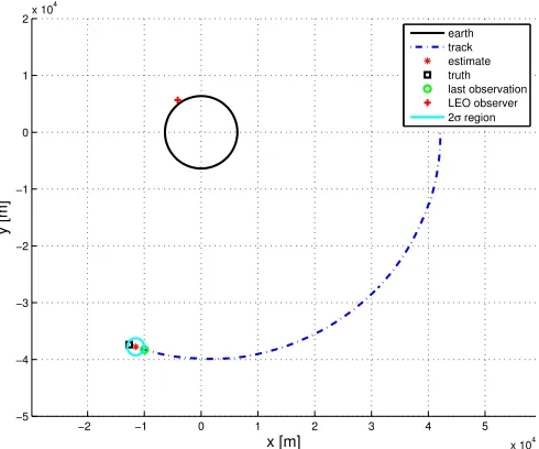
For a benchmark of the parallel implementations we choose a space object tracking problem introduced in [12]. In this problem the object (target) is a satellite in geostationary orbit (GEO) and the measurements are provided by sensors onboard of low Earth orbit (LEO) satellites. The geometry of a typical tracking scenario is illustrated in Fig. 3.1.

Target State Propagation Model

Denote by x(t) the continuous time target state given by

x(t),[r(t) ˙r(t)]0 = [x(t)y(t)z(t)vx(t)vy(t)vz(t)] 0

,

where r(t) and ˙r(t) are the position and velocity vectors, respectively. The target dynamics model is

˙

x=f(t,x(t)) +w(t) (3.1) where f(t,x) = [vx vy vz −(µ/r3)x −(µ/r3)y −(µ/r3)z]

0

, r = px2₊_y2₊_z2_{, µ} _{is the}

Earth gravitational constant, and w = [0 0 0 wx wy wz] 0

is a random process noise which accounts for trajectory perturbations, model inaccuracies, and can serve as a simple model of some maneuvering.

Lettkdenote thekth sampling time, fork = 0,1. . ., andxk ,x(tk). After discretization,

the approximate model is

xk=fk(xk−1) +wk (3.2)

wherefk(xk−1),xk−1+

Rtk

(36)

with covariance Qk. Then, the corresponding state transition Markov model, needed for

(2.1a), is given by

p(xk|xk−1) =pwk(xk−fk(xk−1)) =N(xk−fk(xk−1);0, Qk) (3.3)

where _N denotes a multivariate Gaussian PDF.

Measurement Model

The most popular sensor onboard a space satellite is the space-based visible (SBV) sensor which uses visible band electro-optical camera to measure the azimuth and elevation of a target within the sensor’s field of view. Here, for the purpose of the simulation study, it is assumed more generally that sensors onboard LEO satellites can provide the following type of measurements: range, azimuth, and elevation, defined below.

Range: h(i)

r =

q

(x₋x(i)₎2_{+ (}_y₋_y(i)₎2_{+ (}_z₋_z(i)₎2 _(3.4)

Azimuth: h(i)

a = tan −1

y₋y(i)

x−x(i)

(3.5)

Elevation: h(i)

e = tan −1

 

z₋z(i)

q

(x₋x(i)₎2_{+ (}_y₋_y(i)₎2



 (3.6)

where x(i)_{, y}(i)_{, z}(i)

is thei-th observer location (known), and (x, y, z) is the target location. The measurement model (with the observer’s index omitted) is given by

zk =hk(xk) +vk (3.7)

wherehk(xk),[hr(xk)ha(xk) he(xk)] 0

andvk is zero-mean WGN with covariance Rk which

(37)

(2.1b), is given by

p(zk|xk) = pvk(zk−hk(xk)) =N(zk−hk(xk);0, Rk) (3.8)

Experiment Setup

The simulated benchmark scenario includes a single LEO observer that tracks a GEO satellite in non-maneuvering mode of motion. The LEO orbit is nearly circular with a radius of 6600km and its position is assumed to be accurately calibrated by the GPS. The target being tracked is in a GEO with radius approximately 42164km. Range, azimuth and elevation measurements of the target are simulated without false alarm or missed detection except when the line of sight between the observer and the target is blocked by the earth. The standard deviations of measurement error (matrix Rk) are 0.1km, 2mrad/sec, 2mrad/sec,

for range, azimuth, elevation, respectively. The sensor onboard the observer has a fixed sampling rate of 0.02Hz. For simplicity, both the observer and the target share the same orbit plane. The target has white process noise with the magnitude of random acceleration (matrix Qk) at 0.01m/s2. Fig. 3.1 illustrates the tracking scenario after 500 iterations.

(38)

−2 −1 0 1 2 3 4 5 x 104 −5 −4 −3 −2 −1 0 1 2x 10

4 x [m] y [m] earth track estimate truth last observation LEO observer 2σ region

Figure 3.1: Target Trajectory Estimation; Single MC Run; 500 Iterations.

Performance Measures – Tracking performance

The accuracy of state estimation for all filters was measured in terms of time averaged root mean square error (TARMSE), defined (for both position and velocity), as follows

T ARM SEm,n =

1

n−m n

X

k=m+1

RM SEk (3.9)

where (for position) RM SEk =

1

M

PM

i=1[(x (i)

k −xˆ

(i)

k )

2_{+ (}_y(i)

k −yˆ

(i)

k )

2_{+ (}_z(i)

k −zˆ

(i)

k )

2_]1/2_,

(39)

Performance Measures – Computational Performance

The computational performance of the parallel PFs was measured in terms of the following measures, commonly used in parallel computing.

Execution time: Tp = Execution time for one iteration using p processors (3.10)

Speedup: Sp = T1

Tp

= Execution time for one iteration using 1 processor

Execution time for one iteration usingp processors (3.11)

Efficiency : Ep = Sp

p =

Speedup

Number of processors used (3.12)

The speedup characterizes thescalability of a parallel algorithm. Ideally, the best speedup is linear, i.e.,Sp =p. The efficiency characterizes how well the processors are utilized. Ideally,

it has values between 0 and 1.

Results & Comparative Analysis

Due to space limitation only most representative results are reported in this dissertation. Fig. 3.2 shows the TARMSE (position and velocity) and execution times of the three filters using p= 64 processors versus the number of particles used. Similar results (not pre-sented here) were obtained for different number of processors, e.g.,p= 1,2,4,16,32,64,128. They all indicated (as illustrated in Fig. 3.2, (a) and (b)) that for the RPA and RNA filters a significant improvement of accuracy is achieved by increasing the number of particles up to 100K, and for the CR filter – up to 150K. As it appears, for practical purposes, no more than 100K particles are needed for this tracking problem if RPA or RNA is used, and no more than 150K – if CR is used, regardless of the number of processors.

(40)

0.5 1 1.5 2 x 105

260 270 280 290 300 310 320 330 340

Number of Particles

[m]

(a) Position TARMSE

Cent RPA RNA

0.5 1 1.5 2

x 105 13.5 14 14.5 15 15.5 16 16.5 17

Number of Particles

[m/s]

(b) Velocity TARMSE

Cent RPA RNA

0.5 1 1.5 2

x 105

0 0.02 0.04 0.06 0.08 0.1 0.12 0.14 0.16 0.18

Number of Particles

[sec]

(c) Execution Time

Cent RPA RNA

(41)

Table 3.1: Execution Times

Number of Particles

50,000 100,000 150,000 200,000

p CR RPA RNA CR RPA RNA CR RPA RNA CR RPA RNA

1 0.5554 0.4492 0.3659 1.1165 0.9056 0.7326 1.6794 1.3551 1.0983 2.2455 1.8067 1.4708

2 0.4166 0.3430 0.2815 0.8374 0.6915 0.5636 1.2596 1.0348 0.8449 1.6841 1.3797 1.1314

4 0.2777 0.2368 0.1759 0.5582 0.4775 0.3522 0.8397 0.7145 0.5280 1.1228 0.9526 0.7071

8 0.1157 0.1021 0.0880 0.2326 0.2058 0.1761 0.3499 0.3080 0.2640 0.4678 0.4106 0.3536

16 0.0716 0.0490 0.0416 0.1449 0.0987 0.0831 0.2123 0.1469 0.1243 0.2881 0.1937 0.1665

32 0.0542 0.0268 0.0206 0.1057 0.0515 0.0410 0.1588 0.0740 0.0612 0.2127 0.0979 0.0815

48 0.0462 0.0205 0.0148 0.0923 0.0401 0.0280 0.1395 0.0550 0.0417 0.1865 0.0684 0.0546

64 0.0458 0.0206 0.0119 0.0891 0.0325 0.0219 0.1305 0.0444 0.0318 0.1776 0.0545 0.0420

80 0.0476 0.0197 0.0100 0.0876 0.0299 0.0179 0.1295 0.0385 0.0261 0.1721 0.0474 0.0344

96 0.0473 0.0216 0.0091 0.0877 0.0283 0.0155 0.1313 0.0360 0.0222 0.1746 0.0439 0.0293

112 0.0494 0.0205 0.0085 0.0893 0.0294 0.0142 0.1310 0.0330 0.0197 0.1752 0.0420 0.0254

128 0.0508 0.0260 0.0102 0.0925 0.0311 0.0155 0.1343 0.0336 0.0189 0.1772 0.0404 0.0237

144 0.0528 0.0266 0.0099 0.0954 0.0312 0.0147 0.1351 0.0385 0.0184 0.1834 0.0419 0.0230

160 0.0543 0.0287 0.0095 0.0937 0.0326 0.0138 0.1353 0.0374 0.0178 0.1794 0.0435 0.0223

176 0.0562 0.0308 0.0087 0.0964 0.0338 0.0129 0.1403 0.0395 0.0164 0.1810 0.0406 0.0207

understanding that the CR has the best utilization of particles because it implements the resampling exactly , and the RPA is less approximate than RNA. The differences in accuracy are (somewhat surprisingly) considerable. Quantitatively (based on all simulations with 150K particles), the CR filter is about 10% more accurate than the RPA filter, and the RPA filter itself is about 6% more accurate than the RNA filter. On the other hand, Fig. 3.2, (c) shows the execution time – the “price” paid to achieve the accuracies shown in Fig. 3.2, (a) and (b). Now the order of performance is reversed with the CR filter being significantly slower than the two other filters. Quantitatively (based on all simulations with 150K particles), the CR filter is more than 3 times slower than the RPA filter, and the RPA filter is about 40% slower than the RNA.

(42)

Table 3.2: Computational Performances; 100K Particles

p= 1 2 4 8 16 32 64 96 128 176

Tp 1.1165 0.8374 0.5582 0.2326 0.1449 0.1057 0.0891 0.0877 0.0925 0.0964

Cent SP 1.0000 1.3333 2.0000 4.8000 7.7053 10.5650 12.5320 12.7365 12.0673 11.5843

Ep 1.0000 0.6667 0.5000 0.6000 0.4816 0.3302 0.1958 0.1327 0.0943 0.0658

Tp 0.9030 0.6895 0.4761 0.2052 0.0977 0.0486 0.0302 0.0281 0.0315 0.0334

RPA SP 1.0000 1.3095 1.8966 4.4000 9.2376 18.5841 29.8918 32.1571 28.6954 27.0579

Ep 1.0000 0.6548 0.4741 0.5500 0.5774 0.5808 0.4671 0.3350 0.2242 0.1537

Tp 0.7326 0.5636 0.3522 0.1761 0.0831 0.0410 0.0219 0.0155 0.0155 0.0129

RNA SP 1.0000 1.3000 2.0800 4.1600 8.8178 17.8831 33.3961 47.3319 47.3918 56.6979

Ep 1.0000 0.6500 0.5200 0.5200 0.5511 0.5588 0.5218 0.4930 0.3702 0.3221

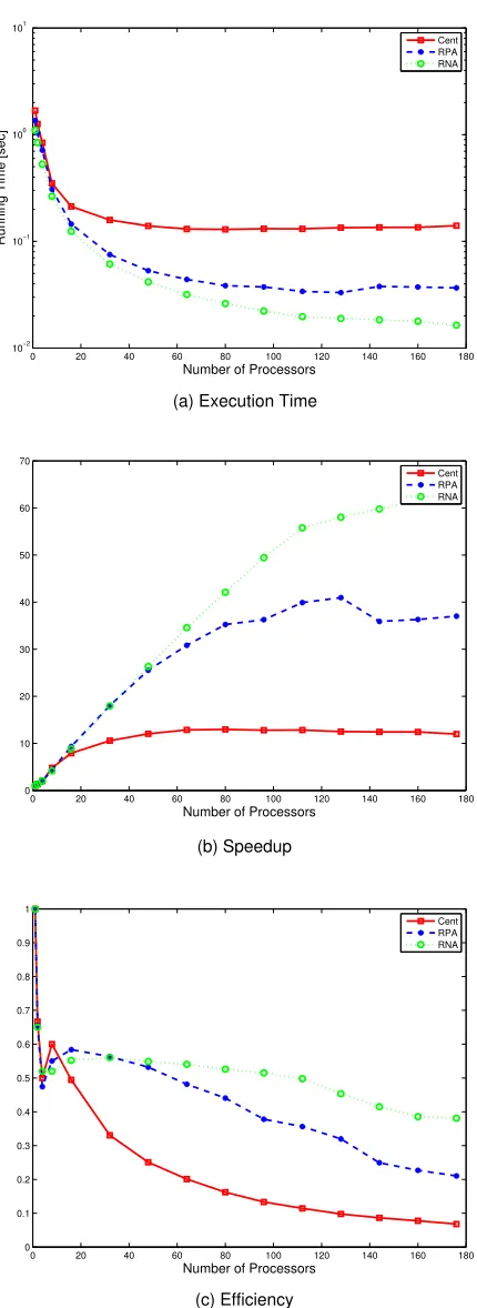
speedup remains constant for p_≥50. Evidently, using CR PPF on more than 50 processors is of almost no use for this problem – most of the effort will be wasted on communication and synchronization. Second, the RPA PPF has significantly better parallel performance than CR. Practically, it provides and effective speedup (good scalability) up to the limit of about 110 processors with a reasonable (about 40%) efficiency within this limit. And, third the RNA PPF is considerably better than the RPA filter in terms of parallel performance. Quantitatively, its effective speedup limit (good scalability) is considerably higher – about 170 processors with about 45% efficiency within this limit.

3.2.3 Case Study II: Ground Multitarget Tracking using Image

Sensor

(43)

0 20 40 60 80 100 120 140 160 180 10−2

10−1 100 101

Number of Processors

Running Time [sec]

(a) Execution Time

Cent RPA RNA

0 20 40 60 80 100 120 140 160 180

0 10 20 30 40 50 60 70

(b) Speedup

Cent RPA RNA

0 20 40 60 80 100 120 140 160 180

0 0.1 0.2 0.3 0.4 0.5 0.6 0.7 0.8 0.9 1

(c) Efficiency

Cent RPA RNA

(44)

three techniques are implemented and experimented on a cluster for resampling – Central-ized Resampling (CR), distributed Resampling with Proportional Allocation (RPA) and distributed Resampling with Nonproportional Allocation (RNA) [10], respectively. Another issue addressed is the inherent interdependence of the partitioning methods for JMPD track-ing. Parallel versions of Independent Partition (IP), Coupled Partition (CP) and Adaptive Partition (AP) are developed and implemented that complete the design of several parallel PF algorithms for JMPD multitarget tracking.

Comprehensive experimentation by simulation of the algorithms over large-scale multi-target tracking scenarios (up to 50 multi-targets) is conducted for performance evaluation. An analysis and comparison is made based on the obtained experimental data. The choice of the “best” among the six compared parallel particle filters for the considered multitarget tracking problem, taking into account the tracking and computational performances, im-poses a complicated trade-off. In this regard, the obtained quantitative experimental results provide helpful information and guidelines in a practical design.

JMPD Particle Filter

In the JMPD approach to multiple target tracking [51, 52, 50, 65, 66, 49] the uncertainty about the number of targets present in a surveillance region as well as their individual states is represented by a single composite PDF. That is, the state of all targets is described by a meta-target state vector Xk = x1k, x2k, . . . , xTk

where xi

k is the state of target i = 1, . . . , T.

(45)

distribution of interest1 _is

p(Xk, Tk|Zk) = p(Xk|Tk, Zk)p(Tk|Zk)

where Zk ₌ _{_Z

1, Z2, . . . , Zk} is the cumulative measurement set of the surveillance region

up to time k, and Zl, l = 1, . . . , k is the measurement set at time l. The model of target

state and number evolution over time is given by p(Xk, Tk|Xk−1, Tk−1) and is referred to as

the kinematic prior. It includes models of target motion, target birth and death, and any additional prior information on kinematics that may be available, e.g., terrain and road maps. The measurement model over the surveillance region is given by the likelihoodP(Zk|Xk, Tk).

For the purpose of our implementation and performance study we adopt the kinematic prior and measurement models of [52].

Each target i= 1, . . . , T is assumed to follow a nearly constant velocity motion model

xi

k=F x i

k−1 +w

i

k (3.13)

where x = (x,˙x,y,˙y)0 _{is the state vector,} _w _{∼ N}₍₀_{, Q}_{) is white process noise with given}

covariance, and

F =diag

        1 ∆ 0 1   ,    1 ∆ 0 1        

where ∆ is the sampling interval. To account for maneuvers a mode variable can be also added [66]. The number of target is considered constant and known. Unknown number of targets using the transitional model of [66] will be included in future work.

It is assumed that a pixelized sensor provides raw (unthresholded) measurements data

1 _{Note that in this formulation the so-called “mixed labeling” [7] is not addressed. It is assumed that no}

track extraction is needed and, consequently, the ordering of xi _within_X _{is irrelevant as far as only the}

(46)

from the surveillance region according to the followingassociation-free model [52] used often for track-before-detect (TBD) problems. A sensor scan at time k consists of the outputs of

M pixels (cells of the region), i.e., Z =_{z[1], . . . , z[M]_}2 _where _z_[_i_{] is the output of pixel}_i_.

The likelihood P(Z_|X, T) is given by

P(Z|X, T)∝ Y

i∈iX

pn[i](X)(z[i])

p0(z[i])

(3.14)

where iX is the set of all pixels that couple to X, n[i](X) is the occupation number of pixel

i (number of targets from X that lie in i). The output z of each pixel is assumed to follow the Rayleigh model

pn(z) = z

1 +nλexp

− z

2

2 (1 +nλ)

, n= 0,1,2, . . . (3.15)

where λ denotes the signal-to-noise ratio (SNR).

With the definition of the transitional densityp(Xk, Tk|Xk−1, Tk−1) and likelihoodP(Zk|Xk, Tk)

the solution to the multitarget tracking problem formally boils down to the BRF (1.1) and the standard SIS/R PF given above can be applied. However, with large number of target the computation requirements become prohibitive. The first step to improve the efficiency of the multitarget PF is to choose an appropriate importance (proposal) distribution for sam-pling that takes into account the specifics of the multitarget problem. Along with the SIR algorithm’s Kinematic Prior (KP) proposal π = p(Xk, Tk|Xki−1, Tki−1), where i− particle

index, [52] suggested three more sophisticated schemes for choosing the importance distribu-tion for multitarget PF, referred to as Independent Partition (IP), Coupled Partition (CP), and Adaptive Partition (AP) [52]. The second step is to parallelize as much as possible the resulting multitarget algorithms. In the next section we develop parallel implementation of

(47)

these schemes and incorporate them in the parallel structures of the corresponding overall multitarget parallel algorithms.

JMPD Parallel PF

In the JMPD SIR PF the proposal is just the kinematic prior and the IS step is completely decoupled with respect to particles _{Xi_}_{. Consequently, all three versions of the above}

generic parallel PF work without any modification. The significantly more efficient proposal schemes IP, CP, and AP of JMPD PF have intrinsic coupling among particles introduced by the dependence of the proposal on the current measurement data. By more careful inspection, however, IP and CP can be parallelized as given next.

Each particle i for Ti targets is Xi =

xi,1_{, x}i,2_{, . . . , x}i,Ti k

and xi,j _{is referred to as a}

partition j of particle i.

The IS step of the JMPD with IP can be done as follows: A) For each partition j = 1, . . . , Ti

k (in parallel) xij_k, wij_k = IP_{xij_k₋₁, w_kij₋₁_}N

i=1, Zk

B) For each particle 1 = 1, . . . , N

Importance weights w_ei

k =wki−1

p(Zk|Xik) ΠT

θ=1w

ij k

where IP denotes the IP subroutine of [52] which practically implements the SIR algorithm for each partition. The IS step of the JMPD with CP can be done similarly, except for IP

being replaced by a subroutine CP which practically implements the known auxiliary SIR particle filter [30] for each partition but only outputs one resampled partition.

The local importance weights wi,j_k are data dependent and their inclusion in the calcu-lation of importance weights w_ei

k amounts to improving the proposal π – bias the proposal

(48)

Part A) can be integrated easily with any of above resampling schemes, CR, RPA, RNA. In the CR version part B) is naturally computed in HN where all particles are resampled. In RPA and RNA versions part B) can also be computed at HN at the expense of an extra communication between HN and all PNs, or it can be computed locally at each PN but this incurs extra pairwise (node-to-node) communication between all PNs. The latter option is parallel but not necessarily faster due to the communication overhead. In our cluster implementation we use the former option – compute B) at HN.

The IP method relies on exact labeling and is only appropriate for well separated (uncou-pled) targets. the CP is appropriate for closely spaced (cou(uncou-pled) targets but is an expensive overkill if targets are not close. Anadaptive partition (AP) can be achieved by spatial clus-tering of the individual partitions and applying IP and CP for the groups of independent and clustered partitions, respectively. In [52] this is achieved by using the K-means clustering algorithm, however, for many targets its sequential implementation (at the head node) is computationally prohibitive.

Implementation on Computer Cluster

We used the cluster computer system Poseidon, housed at the University of New Orleans.

Poseidon is a 128-node, 2 dual-core processor Red Hat Enterprise Linux (RHEL) v4 cluster from Dell with 2.33 GHz Intel Xeon 64bit processors and 4 GB RAM per node. It has 4.772 TFlops peak performance. It is part of the High Performance Computing (HPC) Louisiana Optical Network Initiative (LONI). More technical and performance details of this cluster can be found at URL: http://www.hpc.lsu.edu/systems/.

(49)

The first MPI routine called in any MPI program is the initialization routine MPI INIT. In our implementation the head node (HN) executes function master(), and a processing node (PN) executes function slave(). A high-level pseudo-code of the implemented PPF

with CR, RPA, and RNA, respectively is the same as in Case Study I.

Experiment Setup

The simulated multiple target tracking examples are based on the ground target tracking example of [52]. The targets move in a 5000m_×5000m surveillance area. They have a nearly constant velocity motion, according to (3.13) with Q = diag_{20,0.2,20,0.2_}. The initial position of each target, for each Cartesian coordinate x and y, is generated randomly from the uniform distribution _U(0,5000), and the initial velocity of each target is also generated randomly from the uniform distribution _U(₋10,10). The sensor scans a fixed rectangular region of 50_× 50 pixels, where each pixel represents a 100m_×100m area on the ground plane. The sensor returns Rayleigh-distributed (given by (3.15)) measurements in each pixel, depending on the number of targets that occupy the pixel according to the measurement model (3.14). The sensor sampling interval ∆ = 1s. The presented results are for SNR

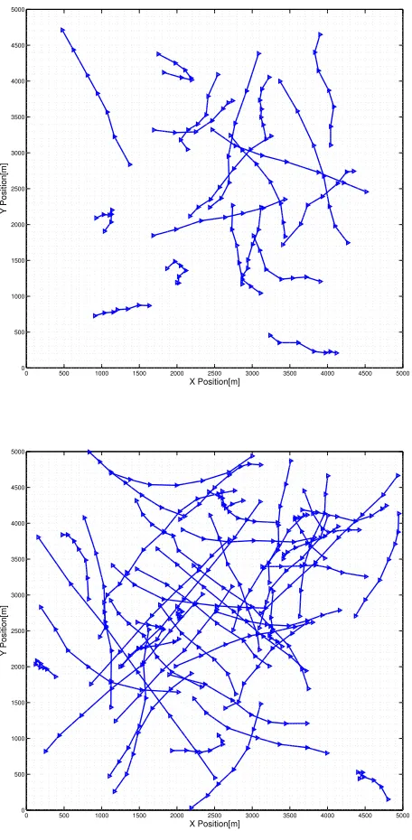
λ= 15. Scenarios with different number of targets were simulated, i.e., T = 3,10,20,30,50. The scenarios with T = 20 and T = 50 are illustrated in Fig. 3.4. The design parameter

(50)

0 500 1000 1500 2000 2500 3000 3500 4000 4500 5000 0

500 1000 1500 2000 2500 3000 3500 4000 4500 5000

X Position[m]

Y Position[m]

0 500 1000 1500 2000 2500 3000 3500 4000 4500 5000 0

500 1000 1500 2000 2500 3000 3500 4000 4500 5000

X Position[m]

Y Position[m]

(51)

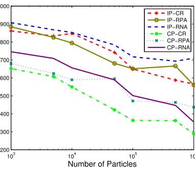
103 104 105 106 200

300 400 500 600 700 800 900 1000

Number of Particles

IP−CR IP−RPA IP−RNA CP−CR CP−RPA CP−RNA

Figure 3.5: Position TARMSE; 64 Processors; 50 Targets; 100 MC Runs.

Performance Measures – Tracking performance

The accuracy of state estimation for all filters was measured in terms of time averaged root mean square error (TARMSE) [46], defined (for both position and velocity) by (3.9), where (for position)

RM SEk=

1

M M

X

i=1

[(x(_ki)₋xˆ_k(i))2_{+ (}_y(i)

k −yˆ

(i)

k )

2_]

!1/2

(3.16)

where i= 1, . . . , M denotes the ith MC run. Likewise for velocity.

The state estimates for each target needed in (3.16) were obtained through K-means clustering of all posterior samples, as suggested by [52], and then computing each estimate as the sample mean of the particles within each cluster.

Performance Measures – Computational Performance

(52)

103 104 105 106 0

5 10 15 20 25 30 35 40

Number of Particles

Running Time[s]

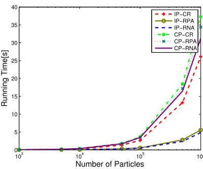
Figure 3.6: Average Execution Time; 64 Processors; 50 Targets; 100 MC Runs.

Results & Comparative Analysis

Due to space limitation, only the most representative results are reported in this dissertation. Included are the following six parallel multitarget tracking algorithms:

IP-CR IP-RPA IP-RNA CP-CR CP-RPA CP-RNA

where IP and CP denote independent and coupled partition, respectively, and CR, RPA and RNA denote centralized resampling, resampling with proportional allocation and re-sampling with nonproportional allocation, respectively. More results are presented for the most difficult 50-target scenario Note that for T = 50 the dimension of the state vector is 200.

Fig. 3.5 shows the position TARMSE and Fig. 3.6 shows the execution times of the six filters using p= 64 processors versus the number of particles used. Similar results (not pre-sented here) were obtained for different number of processors, e.g.,p= 1,2,4,8,16,32,64,128,

(53)

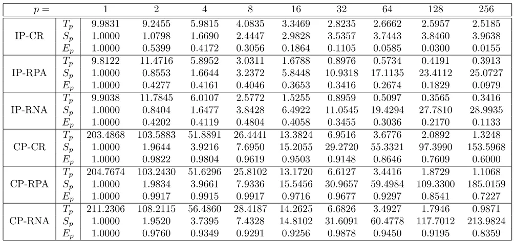
Table 3.3: Execution Time(s); 50 Targets

Number of Particles

10,000 100,000

p IP-CR IP-RPA IP-RNA CP-CR CP-RPA CP-RNA IP-CR IP-RPA IP-RNA CP-CR CP-RPA CP-RNA 1 0.9921 0.9883 0.9999 20.2018 20.3858 20.2411 9.9831 9.8122 9.9038 203.4868 204.7674 211.2306 2 0.9393 1.1786 1.2232 10.3009 10.3325 10.6168 9.2455 11.4716 11.7845 103.5883 103.2430 108.2115 4 0.5910 0.5894 0.6277 5.1990 5.2394 5.3241 5.9815 5.8952 6.0107 51.8891 51.6296 56.4860 8 0.4273 0.2885 0.2440 2.6219 2.6005 2.6810 4.0835 3.0311 2.5772 26.4441 25.8102 28.4187 16 0.3349 0.1759 0.1575 1.3376 1.3371 1.3784 3.3469 1.6788 1.5255 13.3824 13.1720 14.2625 32 0.2930 0.1057 0.0962 0.6964 0.6754 0.6767 2.8235 0.8976 0.8959 6.9516 6.6127 6.6826 64 0.2691 0.0797 0.0784 0.4093 0.3717 0.3695 2.6662 0.5734 0.5097 3.6776 3.4416 3.4927 128 0.2644 0.0977 0.0929 0.2414 0.2084 0.2021 2.5957 0.4191 0.3565 2.0892 1.8729 1.7946 256 0.3273 0.1313 0.1081 0.1727 0.2102 0.1997 2.5185 0.3913 0.3416 1.3248 1.1068 0.9871

Fig. 3.5 also illustrates that CP-CR is the best in terms of accuracy (for the same number of particles), followed by CP-RPA and CP-RNA. This agrees with 1) the understanding that CP is the right partition method to use because the targets are closely spaced and IP is inadequate, and 2) that CR has better utilization of particles than RPA and RNA because it implements the resampling exactly as opposed to RPA and RNA which are approximate. The differences in accuracy are considerable. Quantitatively (based on all simulations with 100K particles), CP-RPA and CP-RNA are about 20% less accurate than CP-CR, and all IP methods are more than 40% less accurate than CP-CR.

On the other hand, Fig. 3.6 shows the execution time – the “price” paid to achieve the accuracies shown in Fig. 3.5. Now the order of performance is reversed with RNA and IP-RPA being significantly faster than all other filters. Quantitatively (based on all simulations with 100K particles - see Table 3.3), IP-RNA and IP-RPA (which are close in computation) are about 4.5 times faster than IP-CR and more than 6 times faster than CP-CR, CP-RPA, CP-RNA which are relatively close in computation time.

(54)

Table 3.4: Computational Performances; 100K Particles, 50 Targets

p= 1 2 4 8 16 32 64 128 256

Tp 9.9831 9.2455 5.9815 4.0835 3.3469 2.8235 2.6662 2.5957 2.5185

IP-CR Sp 1.0000 1.0798 1.6690 2.4447 2.9828 3.5357 3.7443 3.8460 3.9638

Ep 1.0000 0.5399 0.4172 0.3056 0.1864 0.1105 0.0585 0.0300 0.0155

Tp 9.8122 11.4716 5.8952 3.0311 1.6788 0.8976 0.5734 0.4191 0.3913

IP-RPA Sp 1.0000 0.8553 1.6644 3.2372 5.8448 10.9318 17.1135 23.4112 25.0727

Ep 1.0000 0.4277 0.4161 0.4046 0.3653 0.3416 0.2674 0.1829 0.0979

Tp 9.9038 11.7845 6.0107 2.5772 1.5255 0.8959 0.5097 0.3565 0.3416

IP-RNA Sp 1.0000 0.8404 1.6477 3.8428 6.4922 11.0545 19.4294 27.7810 28.9935

Ep 1.0000 0.4202 0.4119 0.4804 0.4058 0.3455 0.3036 0.2170 0.1133

Tp 203.4868 103.5883 51.8891 26.4441 13.3824 6.9516 3.6776 2.0892 1.3248

CP-CR Sp 1.0000 1.9644 3.9216 7.6950 15.2055 29.2720 55.3321 97.3990 153.5968

Ep 1.0000 0.9822 0.9804 0.9619 0.9503 0.9148 0.8646 0.7609 0.6000

Tp 204.7674 103.2430 51.6296 25.8102 13.1720 6.6127 3.4416 1.8729 1.1068

CP-RPA Sp 1.0000 1.9834 3.9661 7.9336 15.5456 30.9657 59.4984 109.3300 185.0159

Ep 1.0000 0.9917 0.9915 0.9917 0.9716 0.9677 0.9297 0.8541 0.7227

Tp 211.2306 108.2115 56.4860 28.4187 14.2625 6.6826 3.4927 1.7946 0.9871

CP-RNA Sp 1.0000 1.9520 3.7395 7.4328 14.8102 31.6091 60.4778 117.7012 213.9824

Ep 1.0000 0.9760 0.9349 0.9291 0.9256 0.9878 0.9450 0.9195 0.8359

provides the computational performances of each filter with 100K particles.

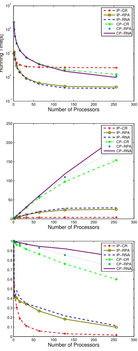
First, based on all results, it is observed that IP-CR has a quite poor scalability and efficiency. Practically, its execution time remains constant for p ≥ 30. Evidently, IP-CR PPF on more than 32 processors is of almost no use for this problem – most of the effort will be wasted on communication and synchronization. Second, IP-RNA and IP-RPA are better than IP-CR but much worse than all CP algorithms in terms of speedup and efficiency. For IP-RNA and IP-RPA there is no real use of increasing number of the processors after

(55)

Finally, Fig. 3.8 provides a comparison of the execution times of the tracking filters as a function of the number of targets.

Summary

In this case study, six parallel particle filters for multitarget tracking have been designed and implemented on a cluster of computers. Comprehensive experimentation by simulation of the algorithms over large-scale multitarget tracking scenarios has been conducted for performance evaluation, and comparison has been made based on the experimental data.

Overall, the CP-CR algorithm is the best in terms of accuracy at a given number of particles and its computation time is close to that of CP-RPA and CP-RNA. CP-RNA and CP-RPA have shown the best computational performance in terms of speedup and efficiency of the parallelization but they do not reduce the computation time of the CP-CR algorithm very significantly. This is because most of the computation time in CP-CR is spent on CP and very little on CR. So, speeding up CR by RPA or RNA with the same number of processors has a little effect on the overall algorithm.

All IP filters are significantly betters in terms of execution time but they have poorer scalability and tracking accuracy than the CP algorithms. RPA and RNA help greatly in reducing the execution time of IP-CR. This is because the resampling is a significant part of the computation with IP and thus RPA or RNA lead to a dramatic reduction of the computation time of the overall algorithm.

(56)

0 50 100 150 200 250 300 10−1 100 101 102 103

Running Time[s] IP−CR IP−RPA IP−RNA CP−CR CP−RPA CP−RNA

0 50 100 150 200 250 300

0 50 100 150 200 250

0 50 100 150 200 250 300

0 0.1 0.2 0.3 0.4 0.5 0.6 0.7 0.8 0.9 1

(57)

0 10 20 30 40 50 0

0.5 1 1.5 2 2.5 3 3.5 4

Number of Targets

Running Time[s]

Figure 3.8: Execution Time; 64 Processors; 100K Particles.

3.3 Improved PF Algorithm for Computer Cluster

3.3.1 Particle Transfer Algorithm (PTA) for Load Balancing

Since the nodes of a computer cluster could communicate with each other easily, we propose to implement an improved algorithm that takes advantage of this capability — the PTA.

The main idea of PTA is to regroup computer nodes based on the weight of each node in order to achieve a better load balancing. It is similar to the RNA described in section 2.1.5 in that the processing nodes (PNs) are grouped, but the groups are adaptively changing in contrast to the RNA wherein the groups are fixed. The weight of each PN is calculated as a sum of the weights of the particles inside the PN, i.e., W =PN

i=1wi. After PN-resampling

Parallel Computing of Particle Filtering Algorithms for Target Tracking Applications

ScholarWorks@UNO

ScholarWorks@UNO

Parallel Computing of Particle Filtering Algorithms for Target

Parallel Computing of Particle Filtering Algorithms for Target

Tracking Applications

Tracking Applications

Acknowledgements

Contents

Abstract

List of Figures

List of Tables

Chapter 1

Introduction

Chapter 2

Background of Related Work

2.1

Particle Filtering

2.1.1

Models

2.1.2

Bayesian Recursive Filter

2.1.3

Basic Particle Filter (PF)

2.1.4

Resampling Algorithms Review

2.1.5

Parallel Resampling

2.2

Particle Flow Filtering

2.2.1

Gaussian Exact Particle Flow Algorithm

2.3

Characterization of Parallel Algorithms

2.3.1

Parallel Algorithms’ Performance Measures

Chapter 3

Parallel Filtering & Tracking

Algorithms for Computer Cluster

3.1

Attributes of Computer Cluster

3.1.1

Message Passing and Communication

3.2

Generic Parallel PF Algorithms for Computer

Clus-ter

3.2.1

Parallelization & Implementation for Computer Cluster

3.2.2

Case Study I: Space Object Tracking

3.2.3

Case Study II: Ground Multitarget Tracking using Image

Sensor

3.3

Improved PF Algorithm for Computer Cluster

3.3.1

Particle Transfer Algorithm (PTA) for Load Balancing