3-D Hydrodynamic and Non-Cohesive Sediment Transport Modeling in the Lower Mississippi River

(1)

University of New Orleans University of New Orleans

ScholarWorks@UNO

University of New Orleans Theses and

Dissertations Dissertations and Theses

Spring 5-16-2014

3-D Hydrodynamic and Non-Cohesive Sediment Transport

Modeling in the Lower Mississippi River

Grecia A. Teran Gonzalez

Civil & Environmental Engineering Department, gterango@uno.edu

Follow this and additional works at: https://scholarworks.uno.edu/td

Part of the Civil Engineering Commons, Environmental Engineering Commons, and the Hydraulic Engineering Commons

Recommended Citation Recommended Citation

Teran Gonzalez, Grecia A., "3-D Hydrodynamic and Non-Cohesive Sediment Transport Modeling in the Lower Mississippi River" (2014). University of New Orleans Theses and Dissertations. 1837.

https://scholarworks.uno.edu/td/1837

This Thesis is protected by copyright and/or related rights. It has been brought to you by ScholarWorks@UNO with permission from the rights-holder(s). You are free to use this Thesis in any way that is permitted by the copyright and related rights legislation that applies to your use. For other uses you need to obtain permission from the rights-holder(s) directly, unless additional rights are indicated by a Creative Commons license in the record and/or on the work itself.

(2)

3-D Hydrodynamic and Non-Cohesive Sediment Transport Modeling in the

Lower Mississippi River

A Thesis

Submitted to the Graduate Faculty of the

University of New Orleans

in partial fulfillment of the

requirements for the degree of

Master of Science

In

Engineering

Civil & Environmental Engineering

by

Grecia Alejandra Terán González

B.S. University of Zulia, Venezuela, 2008

(3)

(4)

DEDICATION

I want to dedicate this achievement to my family,

Migue, Vero and Gabo you opened the doors of your home and took me there for all this time helping me to accomplish this important goal in my life.

Mami, here and in the distance you have always been there to guide me and comfort me.

Migla, you have always believed in me and encouraged me to trust in my potential.

Elio, my love, you were there unconditionally through these years supporting me.

I also wish to dedicate it to my friends,

From the distance, Mate, you always supported me and helped me.

Here, Luis, Tatiana and Sina, you guys became an important part of this journey; you gave me a hand when most needed, among many other invaluable experiences.

(5)

ACKNOWLEDGEMENTS

In first place, I would like to thank Dr. John Alex McCorquodale for giving me the honor of working under his advisory. This opportunity was a blessing for me. I really appreciate all the effort and patience you addressed to teaching me giving me part of your amazing knowledge and wisdom.

This research was funded in part by National Science Foundation (NSF) as a part of the Northern Gulf Coastal Hazards Collaboratory (NG-CHC; http:\\ngchc.org).

I also want to acknowledge Coastal Protection and Restoration Authority (CPRA) for funding part of this research study.

It is also important for me to thank the Lake Pontchartrain Basin Foundation and Dr. John Lopez for providing resources needed in this research study.

I want to thank Deltares for providing me with the software license to carry out this research.

I want to give a special thanks to Dr. Joao Pereira, who was at my first steps in the Master’s program the person who gave me the best advice and taught me the main tools needed to become a modeler. He also helped me overcome, if not solved, many of the problems I faced within my research project. Besides from all of that, he is a good friend, who despite the distance I will never forget.

I also wish to thank Dr. Meselhe for his cooperation and important participation in the development of this study.

I would like to express my gratitude to Dr. Mead Allison for providing me with observed data that was necessary for the accomplishment of this project.

I also want to thank the US Army Corps of Engineers, Gary Brown and Steve Ayers for the observed data.

I want to thank Dr. Chen and Dr. Hu for having the kindness of providing me data for the hurricane runs.

I wish to thank my team workers, Jed and Tshering, mostly during the last stage of this research, for the help.

(6)

LIST OF FIGURES

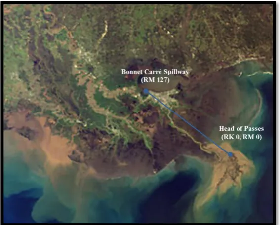
Figure 1. Modeling Domain from Bonnet Carré to Head of Passes (Visible Earth, 2001) ... 1

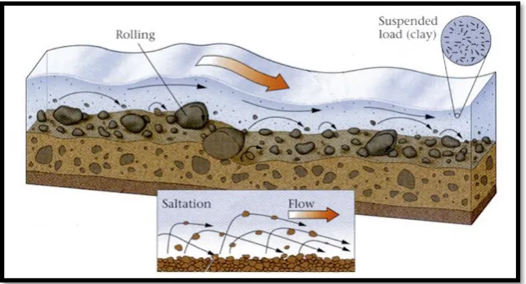
Figure 2. Particle motion mechanisms (UDM, 2013) ... 8

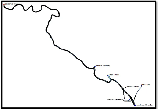
Figure 3. Modeling Domain (USGS, 2007) ... 27

Figure 4. Initial Grid map Indicating Boundary Conditions Type... 28

Figure 5. Transitional Grid map Indicating Boundary Conditions Types ... 29

Figure 6. Final Grid map Indicating Boundary Conditions Types ... 29

Figure 7. Sample importing ... 30

Figure 8. Spline creation ... 30

Figure 9. Grid creation ... 31

Figure 10. Splines deletion ... 31

Figure 11. Refinement and Derefinement ... 32

Figure 12. Grid Ortogonalisation ... 32

Figure 13. Grid Importing into QUICKIN ... 33

Figure 14. Depth and Grid Superposition ... 33

Figure 15. Bathymetry Interpolation... 34

Figure 16. Depth file Generation ... 34

Figure 17. Polygon definition ... 35

Figure 18. Roughness Definition ... 35

Figure 19. Boundary Creation... 36

Figure 20. Boundary Definition ... 37

Figure 21. Final Grid View ... 38

Figure 22. Cuts at Fort St Philip (Google Earth) ... 39

Figure 23. Equivalent Channels at Fort St Philip ... 39

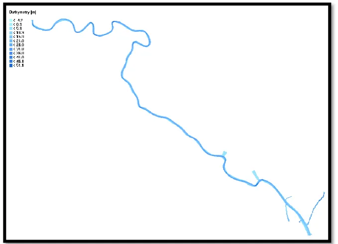
Figure 24. Bathymetry distribution along the domain ... 40

Figure 25. Parabolic Profile for Vertical Layer Distribution ... 40

Figure 26. Manning’s n Roughness distribution along the domain ... 42

Figure 27. Boundaries along the modeling domain ... 43

Figure 28. Original Coarser Grid View ... 45

Figure 29. Original Coarse Grid with Boundary Condition Locations ... 45

Figure 30. Depth varied distribution along the domain for first grid... 46

Figure 31. Simulated and Observed Water Level at Bonnet Carré - March/April 2011 ... 48

Figure 32. Simulated and Observed Water Level at New Orleans - March/April 2011 ... 48

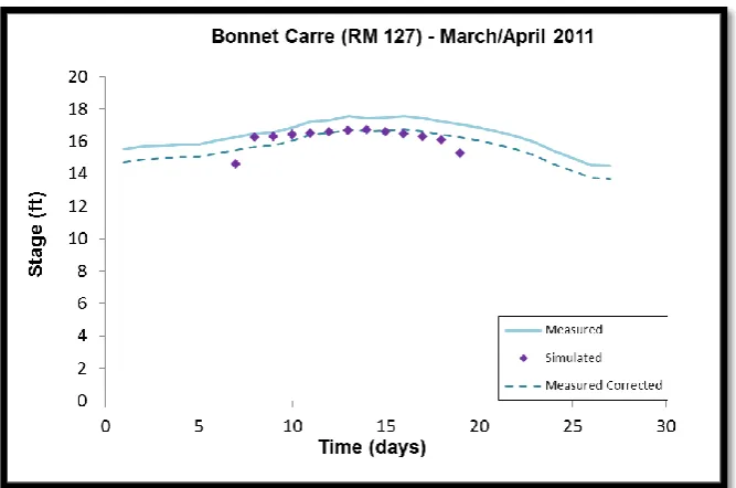
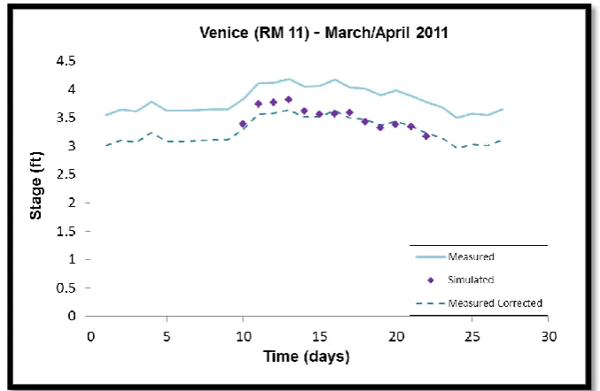
Figure 33. Simulated and Observed Water Level at Venice - March/April 2011 ... 49

Figure 34. Water Level Profile along the Main Channel - March/April 2011 ... 49

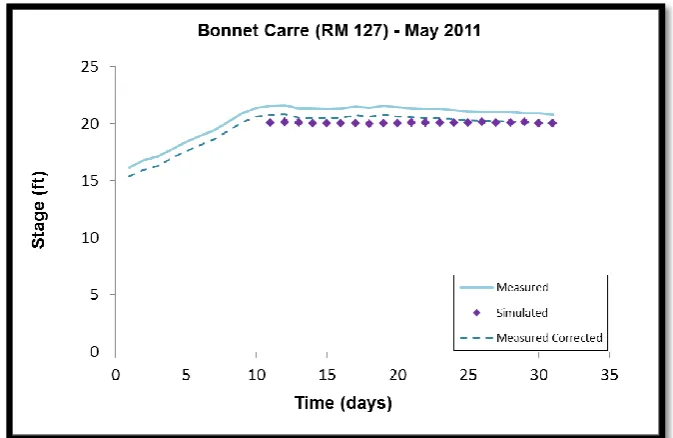
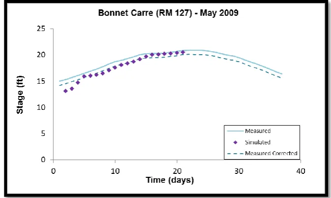
Figure 35. Simulated and Observed Water Level at Bonnet Carré - May 2011 ... 50

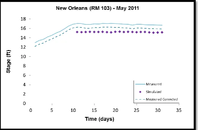
Figure 36. Simulated and Observed Water Level at New Orleans - May 2011 ... 51

Figure 37. Simulated and Observed Water Level at Venice - May 2011 ... 51

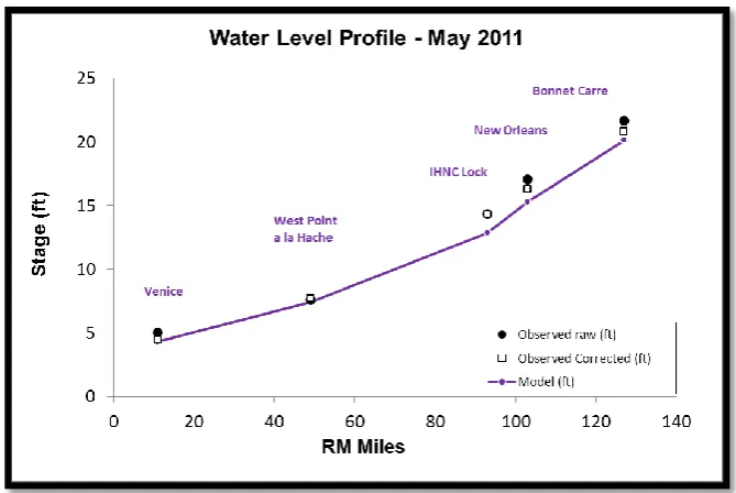
Figure 38. Water Level Profile along the Main Channel - May 2011 ... 52

Figure 39. Simulated and Observed Water Level at Bonnet Carré - May 2009 ... 53

Figure 40. Simulated and Observed Water Level at New Orleans - May 2009 ... 53

Figure 41. Simulated and Observed Water Level at Venice - May 2009 ... 53

(9)

Figure 49. Flow at Fort St Philip – May 2011 ... 58

Figure 50. Estimated and Modeled Discharge for U/S, D/S and outlets – May 2011 ... 59

Figure 51. Model Discharge at Bonnet Carré - May 2009 ... 60

Figure 52. Model Discharge at Head of Passes - May 2009 ... 60

Figure 53. Model Discharge at Fort St. Philip - May 2009 ... 61

Figure 54. Estimated and Modeled Discharge for U/S, D/S and outlets – May 2009 ... 61

Figure 55. Depth averaged velocity map – March/April 2011 ... 63

Figure 56. Depth average velocity map (ft/s) for Myrtle Grove area – March/April 2011 ... 64

Figure 57. Depth average velocity map (ft/s) for Bohemia area – March/April 2011 ... 64

Figure 58. Depth average velocity map (ft/s) for Fort St Philip area – March/April 2011 ... 65

Figure 59. Depth average velocity map (ft/s) for Main Pass area – March/April 2011 ... 65

Figure 60. Depth average velocity map – May 2011 ... 66

Figure 61. Depth average velocity map (ft/s) for Myrtle Grove area – May 2011 ... 67

Figure 62. Depth average velocity map (ft/s) for Bohemia area – May 2011 ... 67

Figure 63. Depth average velocity map (ft/s) for Fort St Philip area – May 2011 ... 68

Figure 64. Depth average velocity map (ft/s) for Main Pass area – March/April 2011 ... 68

Figure 65. Cross-Sectional Velocity Profile, RM 47 – May 2009 ... 69

Figure 66. Vertical Velocity Profile, RM 47 – May 2009 ... 70

Figure 67. Depth average velocity map – May 2009 ... 70

Figure 68. Cross-Sectional Velocity Profile, RM 31 – September 2009 ... 71

Figure 69. Vertical Velocity Profile, RM 31 – September 2009 ... 72

Figure 70. Cross-Sectional Velocity Profile, RM 46 – April 2010 ... 73

Figure 71. Vertical Velocity Profile, RM 46 – April 2010 ... 73

Figure 72. Sediment measurement locations at Myrtle Grove area (RM 61) ... 74

Figure 73. Sediment measurement locations at Magnolia area (RM 47) ... 74

Figure 74. Simulated and Observed Suspended Sand Concentration at Myrtle Grove, MGup2 (RM 61). March/April 2011 ... 75

Figure 77. Simulated and Observed Suspended Sand Concentration at Magnolia, MAG1 (RM 47). March/April 2011 ... 76

Figure 80. Simulated and Observed Suspended Sand Concentration at Myrtle Grove, MGup2 (RM 61). May 2011 ... 78

Figure 83. Simulated and Observed Suspended Sand Concentration at Magnolia, MAG1 (RM 47). May 2011 ... 80

(10)

Figure 86. Simulated and Observed Suspended Sand Concentration at Myrtle Grove, MGup2

(RM 61). May 2011 ... 82

Figure 92. Simulated and Observed Stage at New Orleans (RM 103) for Isaac ... 86

Figure 93. Simulated and Observed Stage at Harvey Lock (RM 98) for Isaac ... 87

Figure 94. Surge height along the Main Channel for Isaac ... 87

Figure 95. Simulated and Observed Stage at New Orleans (RM 103) for Gustav ... 88

Figure 96. Simulated and Observed Stage at West Point a la Hache (RM 49) for Gustav ... 88

Figure 97. Simulated and Observed Stage at Venice (RM 11) for Gustav ... 89

(11)

LIST OF TABLES

Table 1. Model Characteristics for Selection ... 25

Table 2. Manning’s n roughness for main channel ... 41

Table 3. Manning’s n roughness for outlets... 41

Table 4. Sediment Classes, Particle Size and Fall Velocities ... 43

Table 5. Metrics for stage results – March/April 2011 ... 50

Table 6. Metrics for stage results – May 2011... 52

Table 7. Metrics for stage results – May 2009... 54

Table 8. Estimated and Modeled Discharge Values – March/April 2011 ... 57

Table 9. Estimated and Modeled Discharge Values – May 2011 ... 59

Table 10. Estimated and Modeled Discharge Values – May 2009 ... 62

Table 11. Metrics for Velocity Profiles – May 2009 ... 69

Table 12. Metrics for Velocity Profiles – September 2009 ... 71

Table 13. Metrics for Velocity Profiles – April 2010 ... 72

Table 14. Measured and Modeled Bed Load, Suspended Load and Total Load – March/April 2011... 78

Table 15. Measured and Modeled Bed Load, Suspended Load and Total Load – May 2011 . 81 Table 16. Measured and Modeled Bed Load, Suspended Load and Total Load – May 2009 85 Table 17. Metrics for Peak Stage Prediction – Hurricane Isaac ... 87

(12)

LIST OF SYMBOLS

Symbol Description Units

qs Total bed-material load L3/TL

qsb Bed load M/L2

qss Suspended load L2/T

σ Sigma vertical coordinate Dimensionless

z vertical co-ordinate in physical space L ζ free surface elevation above the reference plane L

d depth below the reference plane L

H total water depth L

U depth-averaged velocity in ξ-direction L/T

V depth-averaged velocity in η-direction L/T

√ coefficients used to transform curvilinear to rectangular

coordinates L

√ coefficients used to transform curvilinear to rectangular

coordinates L

Q global source or sink per unit area L/T

qin local source per unit volume T-1

qout local sink per unit volume T-1

P precipitation L/T

E evaporation L/T

Mξ source or sink of momentum in ξ-direction L/T2

Mη source or sink of momentum in η-direction L/T2

u flow velocity in the ξ-direction L/T

v fluid velocity in the η-direction L/T

w fluid velocity in σ-direction L/T

vV vertical eddy viscosity L2/T

vVback background vertical mixing coefficient L2/T

vmol kinematic viscosity (molecular) coefficient L2/T

v3D

part of eddy viscosity due to turbulence model in vertical

direction L2/T

Pξ gradient hydrostatic pressure in ξ-direction M/L2 T2

Pη gradient hydrostatic pressure in η-direction M/L2 T2

Fξ turbulent momentum flux in ξ-direction L/T2

Fη turbulent momentum flux in η-direction L/T2

ω velocity in the σ-direction in the σ-coordinate system L/T

w fluid velocity in σ-direction L/T

P hydrostatic water pressure M/LT2

g acceleration due to gravity L/T2

ρ density of water M/ T3

τ shear stress M/LT2

ρ0 reference density of water M/ T

3

(13)

S source and sink terms per unit area due to discharge T-1

L length L

κ turbulent kinetic energy M2/T2

FL (Ri) damping function

Dk energy dissipation term M2/T3

Pk production term in transport equation for turbulent kinetic

energy

M2/T3

Pkw production term due to wave action M2/T3

Bk Buoyancy flux term in transport equation for turbulent

kinetic energy

M2/T3

ε dissipation in transport equation for turbulent kinetic energy

M2/T3

c’µ constant in Kolmogorov-Prandtl's eddy viscosity

formulation Dimensionless

z’ vertical co-ordinate L

Dw the total depth-averaged due to wave breaking L

ρw density of the water M/ T3

Hrms/2 root-mean-square wave height L

σρ Prandtl-Schmidt number Dimensionless

cD

constant relating mixing length, turbulent kinetic energy

and dissipation in the k- ε model Dimensionless cμ calibration constant Dimensionless

u*b friction velocity at the bed L/T

⃗⃗⃗⃗ vertically averaged friction velocity L/T

Δzb distance to the computational grid point closest to the bed L

z0 bed roughness length L

u*s friction velocity at the free surface L/T

non-dimensional particle diameter Dimensionless

diameter of sediment L

T dimensionless bead shear Dimensionless

τ

bc critical bed shear stress M/LT 2

Cg,90 Chézy coefficient Dimensionless

θcr Shields parameter Dimensionless

reference concentration M/L3

q depth averaged velocity L/T

h water depth L

shape factor Dimensionless

ξc the reference level or roughness height L

zc the suspension number Dimensionless

ε

s (l)

the vertical sediment mixing coefficient for sediment

fraction Dimensionless

ε

f

(l ) _{vertical fluid mixing coefficient} _{Dimensionless}

β Van Rijn’s “beta” factor for the sediment fraction Dimensionless

P wetted perimeter which represents the width L

Q flow rate L3/T

fs silt factor used to incorporate sediment effect Dimensionless

D50 median grain size L

v velocity L/T

(14)

A cross-sectional area L2

Oi observed value -

Pi modeled value -

O average of the observed value - P average of the modeled value -

(15)

ABSTRACT

The purpose of this research is to develop a 3-D numerical model on the Lower Mississippi River to simulate hydrodynamics and non-cohesive sediment transport. The study reach extends from Bonnet Carré Spillway (RM 127) to Head of Passes (RM 0). Delft3D with sigma coordinates was selected as the river modeling tool. This model River domain is characterized by a complex distributary system that connects the Mississippi River to the Gulf of Mexico. The boundary conditions were: water levels in the Gulf and Head of Passes; and discharges upstream. For the calibration, there are observed data for both types of

boundary conditions. Several periods of high discharge were simulated to compare water level, discharge, velocity profiles and sediment transport with measurements and accomplish calibration and validation of the model. A calibrated 3-D model has been developed with the following %RMSE: 5% for stage; 6% for discharge; and 5% for sand load.

(16)

1. INTRODUCTION

1.1 General

The Mississippi River is one of the major rivers of the United States. For centuries it

has been a natural resource that has been used for industrial and economic purposes. As it

approaches the Gulf of Mexico, it creates a large delta, covering approximately 13,000 square

miles. The installation of flood protection systems such as levees, along with dams and

navigation works have negatively affected the replenishment of sediment in the delta. A large

amount of sediment (up to 120 million tons per year) is transported into the Gulf of Mexico

instead of going to the wetlands depriving them of sediment (Allison & Meselhe, 2010;

Parker & Sequeiros, 2006).

The Mississippi River is a complex system and finding solutions to the restoration of

the delta and adjacent wetlands is a very complicated task (CPRA, 2012). However,

numerical modeling can be used as a tool in studying the behavior of the lower Mississippi

River, through the analysis of hydrodynamics and sediment transport along the modeling

domain (Meselhe, et al., 2005).

(17)

This research project presents a three-dimensional model of the Lower Mississippi

River reach extending from Bonnet Carré (RM 127) to the Head of Passes (RM 0) as shown

in Figure 1. Along the reach, there are no mayor inflows but there are numerous outflows

such as West Bay and Main Pass, and the reach downstream of Bohemia (RM 47) on the east

bank of the River where there is a natural levee that overtops in periods of high flow.

This study focuses on the development of a three dimensional numerical model that

predicts the hydrodynamics and the non-cohesive sediment transport on the Lower

Mississippi River. Delft3D (Deltares, 2011), a 3-D finite volume, orthogonal curvilinear grid,

hydrodynamic and sediment transport computer software will be used for the 3-D modeling

of the river domain.

1.2 Problem Statement

The use of computational models to replace physical models to study the

hydrodynamics and sediment transport in environments such as rivers, lakes and coastal areas

is a relatively recent approach but it is a very attractive tool. The computation of solutions for

this kind of model involves solving continuity, momentum and energy equations along with

differential equations for sediment continuity bringing the advantage of adaptability into the

different physical domains compared to what a physical model can provide. Moreover,

numerical models are not subjected to distortion effects as many physical models while being

able to solve the equations for the same flow conditions as the ones observed in the field

(Papanicolaou, Mohamed , Krallis, Prakash, & Edinger, 2008).

The modeling of sediment transport in particular is a very challenging task. It is a very

complex process that requires experimental, field and numerical studies in order to accurately

predict bed load and suspended load, interaction between turbulence, sediment transport in

unsteady flows, among other important parameters (Barkdoll & Duan, 2008).

Furthermore, the Lower Mississippi River is a very unique domain. For high flow

periods, the river bed follows a non-cohesive sediment bed behavior, which must be modeled

under particular formulations in order to calculate erosion and deposition patterns (Pereira,

2011). Under low flow conditions the cohesive sediment regime is more important. Some

issues facing managers of the Lower Mississippi River are: a) river stage and potential

(18)

The effect of new outlets/diversions on these issues requires the predictive capability

of various types of models ranging from 1-D to 3-D models.

The Delft3D-FLOW module (Deltares, 2011) will be used to simulate the

hydrodynamics and non-cohesive sediment transport in the Lower Mississippi River. The

non-cohesive sediment transport simulations will be performed by the implementation of the

Van Rijn (1984) formulation.

1.3 Objective

The main objective of this research project is to develop a Delft3D three dimensional

hydrodynamics and non-cohesive sediment transport model for the Lower Mississippi River

that is capable of simulating the river response to large diversions.

Another important objective is to achieve more independence from other models for

future boundary conditions. This model utilizes stage values as boundary conditions for the

major outlets to the Gulf of Mexico. Stage is preferable to discharge boundary conditions

since is available from monitoring stations and/or sea level rise models.

Finally, the model will be tested for applicability under storm surge hurricane

(19)

2. LITERATURE REVIEW

2.1 Background Research

A three-dimensional morphological sediment transport model was developed by

Lesser et al. using the Delft3D-FLOW module, a multidimensional hydrodynamic and

transport model that calculates non-steady flow and transport phenomena (Deltares, 2011).

Different cases were evaluated, simulating a straight flume, a curved flume and cases applied

to wave and current flume and the Ijmuiden harbor area among other experiments. It was

found on the validation studies a response on different important processes as entrainment,

transport, settling of sediment, varying levels of uniform bed shear stress, bed slope effects,

among others. They also established that further evaluation on the model had to be done due

to some special cases evaluated showing high sensitivity to the bed roughness changes

(Lesser, Roelvink, van Kester, & Stelling, 2004).

A CH3D-SED three-dimensional hydrodynamic model was developed to compute

sediment transport, erosion, and deposition in sand-bed rivers. This model was found to be

well suited for predicting erosion and deposition patterns in bends, distributaries, and thalweg

crossings between bends. The model was validated for the hydrodynamics and sediment

transport simulations for several reaches of the Mississippi River. They found, for instance, at

Red Eye Crossing (RM 223) a 13% difference between their predicted values and

observations for sediment deposition. Moreover, for one of the models, at Head of Passes,

they reproduced successfully the flow distribution, and found good agreement for observed

and predicted velocities and suspended sediment concentrations (Gessler, et al., 1999).

Pereira developed a three dimensional ECOMSED and a one dimensional CHARIMA

unsteady flow mobile-bed model of the Lower Mississippi River from Belle Chasse (RM 76)

to Main Pass (RM 3) to simulate river currents, diversion sand capture efficiency, erosional

and depositional patterns with and without diversions. Also, the introduction of new

diversions at different locations with different geometries and outflows was studied. He

found that the smaller diversions had little impact on the downstream sand transport but

larger diversions had important effects such as the reduction in the slope of hydraulic grade

line, available energy for transport along channels, sand transport capacity in the main

(20)

Upstream of the diversion he found a tendency for erosion and possible head-cutting while

immediately downstream of the diversion there was a zone of deposition (Pereira, 2011).

A 1-D numerical model from Tarbert Landing to the Gulf of Mexico was calibrated,

validated, and applied to predict the response of the Lower Mississippi River to different

stimuli, such as proposed diversions, channel closures, channel modifications, and relative

sea level rise. The model was developed by using HEC-RAS 4.0, a 1-D mobile-bed

numerical model, which was calibrated based on a discharge hydrograph at Tarbert Landing

and a stage hydrograph at the Gulf of Mexico to calculate the hydrodynamics of the river.

The model showed that RSLR will decrease the capacity of the river to carry bed material

(Davis, 2010).

Two one dimensional mobile bed numerical models were set for the Lower

Mississippi River by Gurung (2012). A 1-D HEC-RAS model from Tarbert Landing to the

Gulf of Mexico, based on the 1-D HEC-RAS model developed by Davis (2010); and a 1-D

CHARIMA model from Belle Chasse to the Gulf of Mexico were developed in order to aid in

the restoration and flood control effort. The models were calibrated and validated to predict

the response of the river to channel modifications, varied flow and hurricane conditions. He

observed flow distributions in the un-leveed channels, obtained prediction of shoaling or

erosion in the main stem, and propagation of storm surges and reverse flows under hurricane

conditions (Gurung T. , 2012)

Terán et al. (2013) developed two models to simulate the surge due to Hurricane Isaac

for the Lower Mississippi River, a 1-D HECRAS model from Tarbert Landing to the Gulf of

Mexico and a 2-D Delft3D model from Bonnet Carré to Head of Passes. The period evaluated

represented a very unusual event since the river discharge was near a record low flow and the

storm was moving extremely slow. The 1-D and 2-D models were evaluated for their ability

to accurately predict a hurricane surge in the Mississippi River validating against observed

data obtained from the U.S. Army Corps of Engineers (USACE:rivergages, 2012). Both

(21)

A 2D/3D hydrodynamic and sediment transport model was set up in Yangtze Estuary

region in China. The simulations were run using Delft3D-FLOW. The model was found to be

capable of reproducing the hydrodynamics and sediment transport processes. It was applied

to the storm surge problem and the morphological evolution of Jiuduansha Shoals. It was

found that better results were obtained if wind and wave effects are taken into account for

storm surge simulations; and that the fractions of cohesive and non-cohesive sediment should

be also included to reproduce morphological changes (Hu, Ding, Wang, & Yang, 2008).

A three dimensional model was developed for tidal estuary in the Pontchartrain

Estuary to simulate long term salinity (Retana, 2008). For the development of the model, a

multi-step approach was used involving a physical model of salinity exchange through a pass,

a 3-D FVCOM model of the physical experiment, an FVCOM model of idealized

Pontchartrain Basin and an FVCOM model for the entire estuary, including inputs from the

Mississippi. The model reproduced seasonal salinity. It was also found that a variable friction

coefficient distribution was needed to reproduce tides and salinity and that the model

presented a high sensitivity to this parameter. It was also found that the salinity transport was

improved by implementing a bi-directional open boundary condition in the vertical (Retana,

2008).

2.2 General Concepts

2.2.1 Computational Fluids Dynamics

The analysis of systems involving fluid flow, heat transfer and associated phenomena

based on computer simulations is defined as Computational fluid dynamics (CFD). The

introduction of more advanced high-performance computing hardware and user-friendly

interfaces has promoted to the use of CFD in the solution of many problems including open

channel flows (Versteeg & Malalasekera, 2007).

CFD codes are structured around the numerical features: pre-processor, solver and

post-processor (Versteeg & Malalasekera, 2007). The pre-processing step treats the input of a

flow problem, which involves different activities. One of these is the geometry definition of

the region to be studied, known as the computational domain. Another important task is the

grid generation, which is the subdivision of the domain into smaller, non-overlapping

(22)

Moreover, the phenomena to be analyzed must be selected, the fluid properties must be

defined and appropriate boundary conditions must be specified (Versteeg & Malalasekera,

2007).

The solution process can be done through three numerical solution techniques, which

include: finite difference, finite elements and spectral methods. The finite volume method

represents a special finite difference formulation which involves the integration of a control

volume (employing the divergence theorem to convert some of the volume integrals to

surface integrals) that distinguishes the finite volume method from all other CFD techniques,

and its statements for each finite size cell makes all definitions easier to understand than the

finite element and spectral methods (Versteeg & Malalasekera, 2007).

Finally the post-processing is the final last stage where results are visualized. There

are versatile data visualization tools that allow domain geometry and grid display, plots of

vector, lines and shaded contour, 2D and 3D surface, and also allow particle tracking, view

manipulation (translation, rotation, scaling, etc.) and color PostScript or other graphics output

(Versteeg & Malalasekera, 2007).

2.2.2 Sediment Transport of Non-cohesive Sediment

The transport of sediments by flow of water is the complete transport of solids that

pass through a channel cross section. The sediment transport mechanisms can be explained

by different kinds of motion (Graff, 1998).

There are three main ways in which non - cohesive sediment particles are transported,

which are rolling, suspension and saltation. The rolling motion is given when the bed shear

velocity is slightly greater than the critical bed shear velocity for movement initiation;

suspension takes place when the bed shear velocity is higher than the critical value allowing

the movement of the particle without being in contact with the bed; and saltation occurs when

the bed shear velocity is high enough to allow the particle to travel for a distance without

(23)

Figure 2. Particle motion mechanisms (UDM, 2013)

According to the mechanism of transport the particles that constitute the total bed

material load, qs, can be divided into bed load, qsb, the volumetric discharge per unit width of

rolling particles; and suspended load, qss, the volumetric discharge per unit width of saltating

particles. The total bed material load is defined as the summation of the bed load and

suspended load as follows qs = qsb + qss (Graff, 1998). Some researchers use volumetric

loading units and others use mass loading units.

2.3 Delft3D General Overview

Delft3D is an integrated modeling framework with a multi-disciplinary approach that

can carry out 2-D and 3-D computations for coastal, river, lake and estuarine areas. It can

perform simulations of flows, sediment transports, waves, water quality, morphological

developments and ecology. Delft3D is composed of several modules which are grouped on a

mutual interface being capable to interact with one another. The hydrodynamic simulations

are run with Delft3D -FLOW, a multi-dimensional program that performs unsteady flow and

transport phenomena resulting from tidal and meteorological forcing on a rectilinear or

curvilinear grid. The sigma co-ordinate is used to define the vertical distribution for the three

(24)

2.4 Delft3D Formulation

2.4.1 Hydrodynamic equations

Delft3D-FLOW solves the Navier Stokes equations for incompressible flow. In 3D

models the vertical velocities are computed from the continuity equation. The set of partial

differential equations in combination with an appropriate set of initial and boundary

conditions is solved on a structured grid (Deltares, 2011).

In the horizontal direction orthogonal curvilinear coordinates are used in the Cartesian

system, (ξ, η).

For the vertical direction the system is defined based on the boundary fitting

coordinate system known as the sigma (σ) co-ordinate system which is defined by the

following equation,

(1)

where z is the vertical co-ordinate in physical space; ζ is the free surface elevation

above the reference plane (at z = 0); d is the depth below the reference plane and H is the total

(25)

The vertical σ system presents layers that are bounded by two sigma planes, and that

follow the bottom topography and the free surface. The number of layers remain constant

along the entire domain, however; the distribution of the relative layer thickness can be

variable allowing to give more resolution to the area of interest such as the bed for sediment

transport, among others. For this system we have that the bottom corresponds to σ = -1 and the free surface to σ = 0 as shown in Figure 2 (Deltares, 2011).

The continuity equation is given by:

(2)

where U is the depth-averaged velocity in ξ-direction, V is depth-averaged velocity in

η-direction, and √ √ are coefficients used to transform curvilinear to rectangular

coordinates. With Q representing the contributions per unit area due to the discharge or

withdrawal of water, precipitation and evaporation:

(3)

The momentum equations in the horizontal for the ξ-direction and the η-directionare

given respectively by:

(4)

and

(26)

where u, v, w are the flow velocities in ξ-direction, η- direction and σ –direction

respectively. The three dimensional turbulence is represented by vV, which is the vertical

eddy viscosity defined as:

(6)

vVback is the background vertical mixing coefficient; vmol is the kinematic viscosity of

water and v3D is computed by a 3-D turbulent closure model.

Density variations are neglected, except for the pressure gradients, Pξ and Pη and the

horizontal Reynold’s stresses are represented by the forces Fξ and Fη.

The vertical velocity ω is computed from the continuity equation and it represents the vertical velocity relative to the moving σ-plane. It is define as follows:

(7)

The physical vertical velocities w, which are required for the post-processing, can be

expressed in the horizontal velocities, water depths and vertical ω-velocity according to:

(8)

Under shallow water assumption, the vertical momentum equation is reduced to a

hydrostatic pressure equation given by:

(27)

(10)

For water of constant density and taking into account the atmospheric pressure, the

pressure gradient is defined as:

(11)

(12)

The gradients of the free surface level are the so-called barotropic pressure gradients.

The atmospheric pressure is included in the system for storm surge simulations, since

atmospheric pressure gradients are important in the external forcing at peak winds (Deltares,

2011).

If density is non-uniform, the pressure gradients related to temperature and salinity

effect are defined as:

(13)

(14)

The forces Fξand Fη in the horizontal momentum equations, which represent the

unbalance of horizontal, are expressed as:

(15)

(28)

where τ is the shear stress. For the small-scale flow (partial slip along closed

boundaries), for instance when shear stresses must be taken into account, expressing the shear

stresses as:

(17)

(18)

(19)

For large-scale flow simulated with coarse horizontal grids, for example where shear

stress along the closed boundaries may be neglected, the forces Fξand Fη are simplified as:

(20)



(21)

The discharge of water taking into account momentum adds a term in the U and V

momentum equation:

(22)

(23)

where Mξ is the source or sink of momentum in ξ-direction; Mηis the source or sink of

momentum in η-direction; ̂ is the velocity of water discharged in ξ-direction and ̂ is the

(29)

2.4.2 Transport Equations

The transport of suspended solids, dissolved substances, salinity and heat is often

required in modeling water bodies. The transport is simulated under an advection-diffusion

formulation in three dimensions. In order to represent discharges and withdrawals, the source

and sink terms are included. The transport equation is defined as:

(24)

where DHis the horizontal diffusion coefficient; DV is the vertical diffusion

coefficient; λd represents the 1st order decay process and S is the source and sink terms per

unit area due to discharge (qin) or withdrawal (qout) of water (Deltares, 2011).

2.4.3 Boundary Conditions

A group of initial and boundary conditions for water levels and horizontal velocities

must be specified to get a solution for the 3D and 2D depth-averaged shallow water equations

applied in Delft3D-FLOW. The contour of the model domain consists of closed boundaries which are parts along “land-water” lines (river banks, coastlines) and open boundaries which

are parts across the flow field. Closed boundaries are natural boundaries, while open boundaries are always artificial “water-water” boundaries. To limit the computational area

and computational effort in a numerical model it is necessary to introduce open boundaries.

For Delft3D-FLOW the flow at the open boundaries is sub-critical, which means that

the velocity of wave propagation is bigger than the magnitude of the flow. For subcritical

flow there are two situations, inflow and outflow. At inflow, where the velocity component

along the open boundary is set to zero, it is necessary to specify two boundary conditions

while at outflow it is required to specify one boundary condition. The first boundary

condition is external forced by the water level, the normal velocity, the discharge rate or the

(30)

The reach of the built-in boundary condition is frequently restricted to only a few grid

cells near to open boundary, in that case is recommended to specify the tangential velocity

component, but for Delft3D-FLOW it is not possible yet to specify it at the input, therefore, it

would be suitable to define the model boundaries at locations where the grid lines of the

boundary are perpendicular to the flow with the purpose of obtaining a realistic flow pattern

near the open boundary (Deltares, 2011). This should be accomplished in designing the grid,

since all of the mesh should be orthogonal.

2.4.4 Turbulence

The turbulent scales of motion are solved as a “sub-grid" process since the vertical

and horizontal grid is usually too coarse. The primitive variables are space and time averaged

quantities. Filtering the equations leads to the need for appropriate closure assumptions.

The horizontal eddy viscosity coefficient vHand the eddy diffusivity coefficient DH

are much larger than the vertical coefficients vVand DV. The horizontal coefficients are

assumed to be a superposition of molecular viscosity, 2D-turbulence and 3D-turbulence.

The three-dimensional turbulence is computed following one of the turbulence closure

models. The k-L turbulence closure model is used for the 3-D simulations performed in this

research.

2.4.4.1 k-L Turbulence Model

The к-L model is a first order turbulence closure scheme implemented in

Delft3D-FLOW in which the mixing length L is given by the following equation:

(25)

(31)

The velocity scale is supported on the kinetic energy of turbulent motion. The turbulent kinetic energy к follows from a transport equation that contains an energy

dissipation term Dk, a buoyancy term Bk and a production term Pk, assuming that these terms

are the dominating terms and that the horizontal length scales are much larger than the

verticals ones.

The transport equation is employed in a non-conservative form. The second

assumption leads to simplification of the production term. The transport equation for к is as

follows:

(26)

where Dk is an energy dissipation term, Pk is a production term, Pkw is a production

term due to wave action; Bk is a buoyancy flux term and ε is the dissipation in transport

equation for turbulent kinetic energy .

With,

(27)

The horizontal gradients of the horizontal velocity and all the gradients of the vertical

velocities are neglected in the production term Pk of turbulent kinetic energy, and then this

term is given by:

(28)

A more extended production term Pκ of turbulent kinetic energy (option “partial slip”,

(32)

(29)

In this equation, ν3D is the vertical eddy viscosity, expressed by:

(30)

where c’µ is a constant determined by calibration, derived from the empirical constant

cµ in the κ-ξ model.

In the two previously Pк equations expressed, it has been assumed that the gradients

of the vertical velocity w can be neglected with respect to the gradients of the horizontal

velocity components u and v. In the same way, has been neglected the horizontal and vertical (σ-grid) curvature of the grid.

The turbulent energy production due to wave action is given by Pkw, as is described in

the following equation:

(31)

where z’ is the vertical co-ordinate; Dwis the total depth-averaged due to wave

breaking; ρw is the density of the water; Hrms/2 is the root-mean-square wave height.

(33)

For the к-L model, it is assumed that the dissipation ε depends on the mixing length L

and kinetic turbulent energy к, according to:

(33)

where cD, is a constant determined by calibration, derived from the constant cμ :

(34)

It is necessary to specify boundary conditions to obtain a solution from the transport

equation. It is assumed a local equilibrium of production and dissipation of kinetic energy at

the bed which leads to the following Dirichlet boundary condition:

(35)

To determine the friction velocity u*b at the bed from the magnitude of the velocity in

the grid point nearest to the bed, it is assumed a logarithmic velocity profile, using the

following expression:

(36)

where ⃗⃗⃗⃗ is the vertically averaged friction velocity; Δzb is the distance to the

computational grid point closest to the bed ; z0 is the bed roughness length. The bed

roughness (roughness length) might be improved by the presence of wind generated short

crested waves.

A similar Dirichlet boundary condition is prescribed, in case of wind forcing for the turbulent kinetic energy к at the free surface:

(34)

where u*s is the friction velocity at the free surface. The turbulent kinetic energy k at

the surface is set to zero, in the absence of wind.

At open boundaries, the next equation is used to calculate the turbulent energy k

without horizontal advection:

(38)

For a logarithmic velocity profile this will approximately lead to the next linear

distribution based on the shear-stress at the bed and at the free surface:

(39)

where u*b is the modified friction velocity near bed; u*s is the friction velocity at the

free surface.

2.4.5 Van Rijn (1984)

For the transport of fine sediments without waves, Van Rijn (Rijn, 1984a; 1984b;

1984c) proposes the following relations. The following expression gives the bead – load

transport rate:

(40)

(41)

where is a non-dimensional particle diameter; is the median diameter of

sediment; and T a dimensionless bead shear parameter is calculated with the following

(35)

According to Shields,

τ

bcthis is normalized with the critical bed shear stress using

the following expressions:

(43)

(44)

(45)

where Cg,90 can be defined as the Chézy coefficient, related to the grain and defined

by this expression:

(46)

According to Shields, the critical shear is written:

(47)

From this, θcr defined as the Shields parameter and a function of the dimensionless

particle parameter, obtained with the following expression:

(48)

On the other hand, the expression for the suspended transport is:

(49)

where, is a reference concentration, given by:

(36)

q is the depth averaged velocity; h is the water depth; is the shape factor with

only and approximate solution:

(51)

(52)

where, ξc is the reference level or roughness height (can be interpreted as the bed-load

layer thickness); zc is the suspension number given by:

(53)

(54)

(55)

(56)

“The bed-load transport rate is imposed as bed-load transport due to currents, ,

while the computed suspended load transport rate is converted into a reference concentration

(37)

2.4.6 Non-cohesive sediment dispersion

The vertical sediment mixing coefficient can be calculated using the algebraic or k-L

turbulence model, being computed from the vertical fluid mixing coefficient. When it is non-cohesive sediment, the Van Rijn’s “beta factor” multiplies the fluid mixing coefficient. The beta factor describes the different diffusivity of a fluid “particle” and a sand grain, and the

mathematical representation is:

(57)

where

ε

s (l )

is the vertical sediment mixing coefficient for sediment fraction; β is the

Van Rijn’s “beta” factor for the sediment fraction;

ε

f(l ) is the vertical fluid mixing coefficient

calculated by the selected turbulence closure model (Deltares, 2011).

2.5 Lacey Regime Equations

The Lacey Regime Equations are used for the design of channels, stating a set of stable

channel dimensions for each given flow and silt load (Davis, 2010). The depth and width of

the channel are given based on the wetted perimeter and hydraulic radius.

The width is represented by the expression below,

(58)

The depth of the channel is represented by R which is given by,

(59)

(60)

To estimate the velocity in the channel the next expression is used,

(61)

(38)

(62)

where P is the wetted perimeter which represents the width, ft; Q is the flow rate,

ft3/s; fs is the silt factor used to incorporate sediment effect; D50 is the median grain size, in; v

is the velocity, ft/s; R is the hydraulic radius which represents the depth, ft; A is the

cross-sectional area, ft2.

To obtain the dimensions of the equivalent channels, the cumulative width and depth

of the cuts or bifurcated channels are used.

2.6 Statistical Analysis

The root mean square error (RMSE), the coefficient of determination of r and the bias

between the observations and simulated results were obtained using the following equations:

(63)

(64)

(65)

where Oi is the observed value; Pi is the modeled value; O is the average of the

observed value, P is the average of the modeled value; N is the number of observations

(39)

3. METHODOLOGY

3.1 Model Selection

Different three dimensional models had to be evaluated based on their capabilities

to decide what the best option was for the hydrodynamics and sediment transport simulations

on the modeling domain. After a preselecting process, two models were considered for this

application, mainly based on their availability, ECOMSED and Delft3D.

3.1.1 ECOMSED

ECOMSED is a sigma coordinate, free surface model, designed to realistically

simulate time-dependent distribution of waters levels, currents, temperature, salinity, tracers,

cohesive and non-cohesive sediments and waves in marine and freshwater systems. It is

based on the Princeton Ocean Model developed by Alan Blumberg and George Mellor (1987)

with modifications for its applicability in estuaries and coastal oceans and subsequent

additions from many other contributors. The major assumption in this code and most others is

that the vertical pressure distribution is hydrostatic (McCorquodale & Georgiou, 2006)

3.1.2 Delft3D

Delft3D offers the Delft3D-FLOW module, which is a multidimensional (2D and 3D)

hydrodynamic and transport simulation model which calculates non-steady flow and transport

phenomena resulting from tidal and meteorological forcing on a curvilinear, boundary fitted

domain. In 3D simulations, the vertical grid is defined following the sigma transformation.

This results in a high computing efficiency because of the constant number of vertical layers

over the whole computational domain (McCorquodale & Georgiou, 2006).

3.1.3 Selection Criteria

The model selection criteria are always subjected to the problem that is to be solved

but some common aspects to evaluate are: the availability of the model; what processes can

be simulated; cost of obtaining and implementing the code; assumption and limitations; ease

of utilization; quality of documentation and user manual; hardware and software

requirements; grid system; formulation; graphic user interface; order of accuracy; among

(40)

Based on the most important characteristics to simulate the hydrodynamics and

non-cohesive sediment transport on the Lower Mississippi River, Table 1 is constructed to

visualize in a more practical way which model is more suitable for this purpose.

Table 1. Model Characteristics for Selection

Characteristic ECOMSED Delft3D

Public Domain Yes Yes Distributor HydroQual Deltares

Formulations Finite Volume Method Finite Volume Method Grid Structured Structured Sediment Module Yes Yes

Wetting/Drying No Yes Pre-processing Tool No Yes Post Processing Tool No Yes

Cost Free Free

After analyzing different aspects of models available, Delft3D turned out to be a

more convenient and powerful option to perform the processing, noting that the graphical

user interface provides pre-processing and post-processing tools that ease the modeling

process. The modeled physics are similar in both models.

Delft3D was developed to solve the shallow wave equations in 2-D and 3-D. It has

been successfully applied to coastal areas, estuaries and rivers. It is a public domain model

with a large user group. It was selected for the Mississippi River because it includes: riverine

and estuarine hydrodynamics, sediment transport and channel morphology. It has an excellent

graphics interface (Teran, et al., 2013).

3.1.4 Delft3D Capabilities

The Delft3D main capabilities that are suited for this project research involve:

 3-D hydrostatic numerical model

 Orthogonal curvilinear grid

 Based on a sigma (σ) level coordinates for the vertical distribution

(41)

3.2 General Modeling Setup

A 3-D Delft3D numerical model was developed for hydrodynamics and non-cohesive

sediment transport simulations on the Lower Mississippi River.

3.2.1 General Considerations

The study area extends from Bonnet Carré (RM 127) to the Head of Passes (RM 0).

The model was applied to simulate the hydrodynamics and non-cohesive sediment transport

of the modeling domain for high flow periods. After experimentation with a range of time

steps, the simulations were performed using a time step of 0.5 minutes. The sigma levels

were variable according to a parabolic distribution with the smallest layers near the bed. A

variable roughness was used over the domain. Van Rijn’s 1984 sediment formulations were

used for the sediment transport simulations. The basic model developed at the beginning of

the research project was applied to periods under hurricane storm surge conditions.

3.2.2 Modeling Domain

The modeled reach in this study extends from Bonnet Carré (RM 127) to the Head of

Passes (RM 0), which is shown in Figure 3. Along the reach there are some continuous

outflows such as West Bay and Main Pass, and the east bank of the river downstream of

Bohemia (RM 47) has a natural levee that overtops in periods of high flow. Some other

outlets are: Grand Pass and Tiger Pass, Baptiste Collette, Fort St Philip, Caernarvon and

(42)

Figure 3. Modeling Domain (USGS, 2007)

3.2.3 Model Development

To start up the model, a 2-D depth-averaged model in the study reach was set up

based on a 2-D hydrodynamic model built by Dr. Pereira (Pereira, 2-D Regional Delft3D

model for the Mississippi River Hydro-study, 2012) based on discharge boundary conditions

for all outlets for the same reach. Figure 4 shows the original grid indicating all outlets

boundary conditions being discharge type. First, a uniform bathymetry and uniform

roughness for the main channel and outlets were used. For this stage, the modeled was to be

transformed from a discharge based boundary condition for the outlets to a stage based model

for the most important outlets in the domain. This process had to be done step by step, since

those changes lead to instabilities.

Bonnet Carré RM 127

(43)

Figure 4. Initial Grid map Indicating Boundary Conditions Type

After the main outlets (West Bay, Main Pass, Bohemia Spillway, Grand Pass and

Tiger Pass, Baptiste Collette and Fort St Philip) were set to stage boundary conditions, the

model was converted into a three dimensional model, with 10 layers under a parabolic

scheme, going from thinner layer at the bottom to thicker at the surface. Along with the

conversion to a 3-D model, the bathymetry and roughness Manning’s n were converted to a

variable distribution to obtain a more realistic setting of the model. Figure 5 shows the

(44)

Figure 5. Transitional Grid map Indicating Boundary Conditions Types

Moreover, some overflow zones were extended to account for channels present

between the Bohemia and Fort St Philip area. Figure 6 shows the last grid for the extended

(45)

3.2.3.1 Grid Generation

The generation of the grid by using the Delft3D was a simple but time consuming

process. The tool used for this purposed was the RGFGRID. The grid was built on a map

sample that was imported into the grid generation tool. Figure 7 shows the samples being

imported to the grid generation tool.

Figure 7. Sample importing

The next step consisted in creating splines following the shape of the river section.

Figure 8 displays the spline creation on a section of the main stem of the river.

(46)

After the splines are defined, they must be converted into grid. Figure 9 shows the splines being converted to grid.

Figure 9. Grid creation

Then splines must be deleted, which is shown on Figure 10.

Figure 10. Splines deletion

Depending on the way the splines are drawn, it might be necessary to refine or

(47)

Figure 11. Refinement and Derefinement

Once the grid has been developed, it is necessary to orthogonalise it, this process is shown in Figure 12.

Figure 12. Grid Ortogonalisation

(48)

3.2.3.2 Bathymetry Interpolation

The bathymetry interpolation was done by using the QUICKIN tool. The generated

grid file (.grd) and depth samples (.xyz file) must be imported into the interface. Figure 13

shows the grid being imported into the program, and Figure 14 presents the bathymetry and

the grid being superposed.

(49)

Figure 15. Bathymetry Interpolation

Finally, the depths must be exported as a .dep file to create the bathymetry file, as

displayed in Figure 16.

Figure 16. Depth file Generation

3.2.3.3 Roughness File Generation

The roughness file for a spaced varied distribution is generated using the QUICKIN

tool. As done for the bathymetry interpolation, the grid must be imported to the tool. Once

the grid has been displayed, a polygon around the desired area must be drawn to define the

(50)

Figure 17. Polygon definition

Once the polygon was drawn, the value for the roughness must be defined. Figure 18

shows the option to insert the roughness value, which is created like a depth file.

(51)

Once the .dep file has been exported, an .rgh file must be created containing the

values assigned as depth on this last .dep file. It is important to highlight that the roughness

file needs to be filled with a component on the u direction, and one for the v direction. As

recommended by Deltares, both components were defined with the same value, meaning the

values defined as depth for the roughness are pasted twice on the roughness file.

3.2.3.4 Boundary Condition Definition

The boundary conditions are defined on the Flow input tool. Once the grid has been

generated, the .mdf file (main input file) can be created to define all the variables needed,

including the boundary conditions. The grid file must be imported into this input file. Figure

19 shows the main options on the menu of the .mdf generation file, where the Boundaries

button can be observed. Under this option, using the visualization area, the boundaries are

defined. Figure 20 shows the created boundary.

(52)

Figure 20. Boundary Definition

The flow input tool only allows the specification of two values for each boundary, one

initial and one final value. However, the data were introduced externally on the ASCII file

generated (.bct file).

3.3 Hydrodynamics and Sediment Transport Set up

3.3.1 Grid Resolution

The grid has a varied resolution. The total grid consists of 2004 points in the M

direction and 117 points in the N direction. The main channel consists of about 20 cells

across. The typical grid dimension is 50m. Figure 21 shows a portion of the grid where the

(53)

Figure 21. Final Grid View

3.3.2 Bathymetry

Setting up the bathymetry for this model was a very wearying task. The construction

of the bathymetry file consisted on compiling data from different sources, such as LIDAR

2003 bathymetry data, Corps of Engineers Multibeam, Lake Pontchartrain Basin Foundation

(LPBF) surveyed height of land data and Google Earth data.

The surveyed depths were used to build the bathymetry where available; otherwise,

the depths were estimated by using Lacey Regime equations based on the measured widths of

the channels (Google Earth). For the overflow areas, such as Fort St Philip and Ostrica, some

equivalent channels were used to replace the cuts present in those areas (based on ΣAR2/3)

that have the capability to extract flow from the main channel. Figure 22 displays the

dimensions for the equivalent channels, and Figure 23 shows the bathymetry and the grid

around that area.

Also, the Gras Pass, which is a channel that formed in the Bohemia area during the

(54)

(55)

The bathymetry distribution for the modeling domain is shown in Figure 24.

Figure 24. Bathymetry distribution along the domain

3.3.3 Layer Distribution

The vertical sigma coordinates consist on 10 layers being 11 sigma levels along the

entire domain. They are distributed under a parabolic profile, going from the thinner layer at

the bottom to the thicker one at the surface. Figure 25 shows the vertical profile for the layer

distribution.

(56)

3.3.4 Roughness

The roughness was defined under Manning’s n formulation. It was a varied

roughness along the entire domain. The Manning’s n was the main parameter to calibrate the

hydrodynamics in the model. Tables 2 and 3 present the Manning’s n used in the different

areas of the modeling domain.

Table 2. Manning’s n roughness for main channel

Area – Main Channel Manning’s n

Bonnet Carré (RM 127) to New Orleans (RM 103) 0.02600 New Orleans (RM 103) to IHNC Lock (RM 93) 0.02700 IHNC Lock (RM 93) to West Point a la Hache (RM

49) 0.01680

West Point a la Hache (RM 49) to Bohemia area (RM

44) 0.01450

Bohemia area (RM 44) to Venice (RM 11) 0.01485 Venice (RM 11) to Head of Passes (RM 0) 0.01750

Table 3. Manning’s n roughness for outlets Area – Outlets Manning’s n

Bohemia Spillway 0.06 Bohemia 2 0.06 Ostrica 1 0.08 Ostrica 2 0.07 Equivalent Channels @

Ostrica 0.05 Fort St Philip 0.10 Fort St Philip 2 0.10 Equivalent Channels 0.03 Baptiste Collette 0.03 Grand + Tiger Pass 0.04 West Bay 0.06 Main Pass 0.03 Gras Pass 0.05

Figure 26 displays the Manning’s n roughness distribution map in the modeling

(57)

Figure 26. Manning’s n Roughness distribution along the domain

3.3.5 Boundary Conditions

The upstream boundary condition at Bonnet Carré (RM 127) and Caernarvon and

Davis Pond diversions corresponds to daily discharge flows obtained from a calibrated 1-D

HEC-RAS model from Tarbert Landing to Gulf of Mexico (Gurung T. , 2012). The

downstream end, Head of Passes (RM 0), and outlets (Main Pass, West Bay, Baptiste

Collette, Grand Pass + Tiger Pass, Fort St, Philip and Bohemia Spillway) boundary

conditions consist on daily stage values obtained from USACE data (USACE:rivergages,

2012) and NOAA data (NOAA:Tides&Currents, 2012). The outlets data corresponds to data

at the Gulf of Mexico for the corresponding periods. Figure 27 shows the modeling domain

(58)

Figure 27. Boundaries along the modeling domain

3.3.6 Sediment Transport Main Settings

The sediment transport formulations correspond to the Van Rijn (1984) equations.

Three sediment classes are included based on the particle size. Table 4 shows the grain sizes

and settling velocities corresponding to the different classes of sand particles simulated in the

model.

The sediment size distribution was completed based on a USACE report (Nordin &

Queen, 1992).

Table 4. Sediment Classes, Particle Size and Fall Velocities Sediment

Class

Sediment Size, D50 (mm)

3-D Hydrodynamic and Non-Cohesive Sediment Transport Modeling in the Lower Mississippi River

ScholarWorks@UNO

ScholarWorks@UNO

3-D Hydrodynamic and Non-Cohesive Sediment Transport

3-D Hydrodynamic and Non-Cohesive Sediment Transport

Modeling in the Lower Mississippi River

Modeling in the Lower Mississippi River

3-D Hydrodynamic and Non-Cohesive Sediment Transport Modeling in the

Lower Mississippi River

A Thesis

Submitted to the Graduate Faculty of the

University of New Orleans

in partial fulfillment of the

requirements for the degree of

Master of Science

In

Engineering

Civil & Environmental Engineering

by

Grecia Alejandra Terán González

B.S. University of Zulia, Venezuela, 2008

DEDICATION

ACKNOWLEDGEMENTS

TABLE OF CONTENTS

LIST OF FIGURES

LIST OF TABLES

LIST OF SYMBOLS

τ

ε

ε

ABSTRACT

1.

INTRODUCTION

2.

LITERATURE REVIEW

τ

ε

ε

3.

METHODOLOGY