USING A MODIFIED MONTE CARLO METHOD
By
Michael B. Morse
A thesis
submitted in partial fulfillment of the requirements for the degree of
Master of Science in Materials Science and Engineering Boise State University
DEFENCE COMMITTEE AND FINAL READING APPROVALS
of the thesis submitted by Michael B. Morse
Thesis Title: Effects of Grain Boundary Character on Dynamic Recrystallization Using a Mod-ified Monte Carlo Method
Date of Final Oral Examination: 11 October 2011
The following individuals read and discussed the thesis submitted by student Michael B. Morse, and they evaluated his presentation and response to questions during the final oral examination. They found that the student passed the final oral examination.
Megan E. Frary, Ph.D. Chair, Supervisory Committee Darryl P. Butt, Ph.D. Member, Supervisory Committee Pushpa Raghani, Ph.D. Member, Supervisory Committee
Effects of Grain Boundary Character on Dynamic Recrystallization Using a Modified Monte Carlo Method
Michael B. Morse
Dynamic recrystallization (DRX) is the recrystallization that occurs during high temperature deformation of metals and alloys. While DRX has been observed experimentally, the parameters that affect the microstructure are still being explored. For example, the effects of temperature, strain rate, and initial grain size have already been studied, yet the effect of initial special bound-ary fraction is still unknown. Special boundaries are high-angle, low-energy grain boundaries. It is believed that higher initial fractions of special boundaries will lead to a delay in the onset of recrystallization and a higher peak stress.
Experimentation has shown that triple junctions are preferred nucleation locations for DRX. This work will look at the different types of triple junctions (categorized based on the number of special boundaries at the junction) and determine the effect that special boundaries have on the probability of nucleation. It was supposed that triple junctions without special boundaries would be preferred nucleation sites due to higher grain boundary energy. This work showed that triple junctions sites, particularly triple junctions without special boundaries, were the preferred nucleation location.
ABSTRACT . . . iv
LIST OF TABLES . . . vii
LIST OF FIGURES . . . viii
1 INTRODUCTION . . . 1
1.1 Motivation for Research. . . 1
1.2 Objectives . . . 2
2 BACKGROUND INFORMATION . . . 3
2.1 Grain Boundary Types and Classification . . . 3
2.2 Strain and Stored Energy . . . 8
2.3 Recrystallization . . . 9
2.4 Conditions of Dynamic Recrystallization . . . 10
2.5 Kinetics of Dynamic Recrystallization . . . 12
2.6 Monte Carlo Simulation. . . 14
3 SIMULATION PROCEDURES . . . 16
3.1 Overview of Simulation Process . . . 17
3.2 Grain Boundary Classification . . . 17
3.3 Dynamic Recrystallization. . . 23
3.4 Grain Growth Algorithms . . . 25
4 RESULTS AND DISCUSSION . . . 29
4.1 Initial Microstructure . . . 29
4.3 Temperature Effects . . . 33
4.4 Effect of Special Boundary Fraction . . . 37
4.5 Nucleation Location and Available Nucleation Sites . . . 41
5 CONCLUSIONS . . . 49
5.1 Implications . . . 49
5.2 Future Work . . . 50
REFERENCES . . . 51
Table 3.1 A list of the grain boundaries that are taken into account by the simulation and their assigned energy values. . . 21 Table 3.2 List of grain curvature coefficients. HigherΣboundaries are more mobile and
there-fore the effect of curvature would have a greater effect. . . 28
Table 4.1 Special boundary information for starting microstructure. . . 29
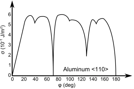
Figure 2.1 DRV is evident by a non-linear stress-strain curve while DRX results in a curve with a portion of the curve having a non-positive slope. . . 5 Figure 2.2 Experimental plot of grain boundary energy as a function of misorientation for
<110> plane in Aluminum.. . . 7 Figure 2.3 A coincident boundary (left) occurs when the boundary coincides with the
twin-ning plane. An incoherent boundary (right) occurs when a boundary intersects the twinning plane at an angleθ. . . . 8 Figure 2.4 Simulated equivalent of a stress-strain curve. The average stored energy in the
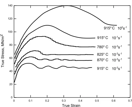
sys-tem indicates which process is dominant: grain growth or recrystallization.. . . . 9 Figure 2.5 A schematic model for the nucleation of a grain at a grain boundary (GB). . . 11 Figure 2.6 Experimental stress-strain curve for 0.68 % C steel. . . 11 Figure 2.7 Each hexagon represents an individual sample site. The varying colors represent the
orientation of the particular tiles and similar orientations are grouped into grains and neighboring grains are separated by a grain boundary, noted here by a thick black line. . . 15
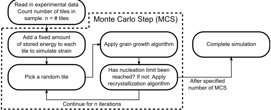
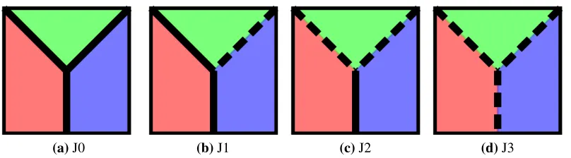
Figure 3.1 A flowchart showing the general concept of what occurs during the simulation. The dashed line represents what operations are performed each Monte Carlo step. . . . 18 Figure 3.2 (a) Shows a triple junction with no special boundaries present, (b) with a single
spe-cial boundary, (c) with two spespe-cial boundaries, and (d) with three spespe-cial boundaries. 22
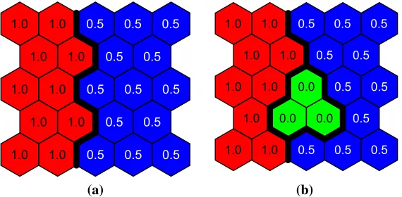
sen and tested to see if it is energetically favorable to nucleate. Should the conditions be favorable to form a nucleus, a strain-free grain is formed and the stored energy is set to zero. (a) shows the initial microstructure and (b) shows the microstructure af-ter a nucleus is formed. Each color represents a separate grain. The numbers within the tiles represent the stored energy. . . 24 Figure 3.4 Schematic of (a) Two neighboring grains (denoted by red and blue colors) with
differing stored energy values. (b) The left grain grows by a single tile (hexagon) and the stored energy of that tile is an average of the two tiles chosen as a possible grain growth site. . . 27
Figure 4.1 Experimentally obtained EBSD scan of 316L Stainless Steel for (a) a sample that has undergone a single GBE cycle and (b) a sample that has undergone three GBE cy-cles. Solid colors represent grain orientation while thin lines represent grain bound-aries. Black grain boundaries are general boundaries while red are Σ3boundaries.
30
Figure 4.2 Simulations of the low-fraction sample showing that increasing the nucleation rate decreases the cyclic behavior for constant temperature and strain rate. Also, higher nucleation rates increase the peak stored energy value and delay the number of Monte Carlo steps where the peak value occurs. The simulation was anisotropic with a strain rate of 0.0002. . . 31
decreases the cyclic behavior for constant temperature and nucleation rate. This also decreases the peak stored energy value, and shortens time until the peak value offurs (i.e., shifts the peak to the left). . . 32 Figure 4.4 Average stored energy for low-fraction sample with accompanying microstructure
maps. The percentage next to the microstructure maps refers to the amount of new grains when compared to the original grains. For example, 25% means that 25% of the original grains have been removed due to grain growth and recrystallization. The various colored grains correspond to various grain orientations while the lines between the grains correspond to grain boundary types. Black lines are general boundaries while red lines are special boundaries.. . . 34 Figure 4.5 Simulations of the expected behavior for (a) and (b) of decreasing average stored
energy with increasing temperature holds true for the simulated results except for exceptionally low strain rates; this trend stands for both the high-fraction and low-fraction samples. . . 35 Figure 4.6 Simulations of the maximum stored energy plotted for each materials at varying
strain rates and temperatures. The effect on the peak average stored energy due to temperature and nucleation rate are greater at higher strain rates. Note that lines are not trend lines. . . 36 Figure 4.7 Comparing rates of recrystallization for isotropic and anisotropic simulations. Both
the low and high-fraction samples showed that recrystallization was delayed for anisotropic simulations when compared to isotropic runs. The delay in recrystal-lization is more pronounced for the high-fraction sample.. . . 38
that the energy peaks for the high-fraction samples are lower and shifted to the right when compared to energy peaks for the low-fraction sample. Physically, this would correspond to an earlier onset of DRX. . . 39 Figure 4.9 Comparing special boundary fraction to (a) the maximum average stored energy
as well as (b) the time required to reach the maximum average stored energy. The data shows that there may be a similar correlation between the effect of special boundaries and the effect of initial grain size: higher special boundary fractions have the potential to have a similar effect as larger initial grain sizes. . . 40 Figure 4.10 Comparison of the effect of forcing a percentage of new nuclei to formΣ3
bound-aries with a random neighbor in both the high- and low-fraction samples. Simu-lations were conducted at the same temperature and strain rate for both samples. Higher percentages of forcedΣ3 boundaries slow the decline of the overall special boundary fraction and increase the steady state fraction. . . 42 Figure 4.11 Comparison of available nucleation sites to the actual location at which nucleation
occurs for the low-fraction sample. The shaded area on the left plot denotes the portion of the simulation dominated by grain growth. Solid bars on right graph denote the fraction of nuclei that formed for each boundary type. Lighter bars denote initial fraction of available nucleation sites of each type at 4,000 MCS. . . 44
ation occurs for the low-fraction sample. The shaded area on the left plot denotes the portion of the simulation dominated by grain growth. Solid bars on right graph denote the fraction of nuclei that formed for each boundary type. Lighter bars de-note initial fraction of available nucleation sites of each type at 4,000 MCS. Only the peak percentage of available J0 sites fails to surpass the corresponding actual nucleation fraction. . . 45 Figure 4.13 Comparison of available nucleation sites to the actual location at which nucleation
occurs for the high-fraction sample. The shaded area on the left plot denotes the portion of the simulation dominated by grain growth. Solid bars on right graph denote the fraction of nuclei that formed for each boundary type. Lighter bars denote initial fraction of available nucleation sites of each type at 4,000 MCS. While the percentage of available triple junction sites never reaches 15%, the percentage of nuclei that formed at a triple junction was closer to 25%. . . 46 Figure 4.14 Comparison of available triple junction sites to the actual location at which
nucle-ation occurs. The shaded area on the left plot denotes the portion of the simulnucle-ation dominated by grain growth. Solid bars on right graph denote the fraction of nuclei that formed for each boundary type. Lighter bars denote initial fraction of avail-able nucleation sites of each type at 4,000 MCS. Higher J-value sites nucleate less favorably. . . 47
1 INTRODUCTION
1.1 Motivation for Research
Dynamic recrystallization (DRX) involves grain growth and simultaneous recrystallization during high-temperature deformation in materials with low stacking fault energies. Prior to 1965, recrystallization was thought to be a process where the grain refinement and reduced strain hard-ening occurred after processing and during annealing only [1]. However, as material characteri-zation techniques improved, it was seen that at certain temperatures and strain rates, grain growth, recrystallization, and an overall reduction of strain hardening occurredduringhigh-temperature material processing and can alter a material’s microstructure. This observation, combined with the discovery that microstructure plays an important role in macroscopic material properties, gave rise to the study of recrystallization during processing, called dynamic recrystallization.
By improving our understanding of DRX, it may be possible to tailor processes and ma-terials to more precisely suit specific applications. This understanding can be aided through the development of realistic simulations of the DRX process. Developing a simulation requires mathematical equations that reflect the physical processes of DRX. This simulation provides a possible outcome that can be validated by applying the same experimental parameters to the ma-terial from which the initial microstructure was obtained. Imaging the mama-terial after physical experimentation can help to validate the observations derived from the simulation.
next section, the implications extend far beyond them, allowing additional investigation into DRX in materials other than stainless steel 316L and nickel.
1.2 Objectives
In the 1980s, the Monte Carlo method was adapted to examine the mechanics of grain growth and nucleation. This method involved converting a sample area into discrete sites that could then be selected at random and algorithms were then applied to simulate specific processes [1, 2]. For this thesis, a modified Q-state Potts model was chosen to simulate DRX using experimentally obtained microstructures [3].
2 BACKGROUND INFORMATION
Dynamic recrystallization involves a combination of grain growth and simultaneous recrystal-lization during high-temperature deformation of metals and alloys. This occurs when a material with an average low- to medium-stacking fault energy is heated to approximately half its melting temperature while being strained in compression, tension, or torsion [1, 4–7]. Recrystallization has been described by R.D. Dohertyet al. [1] as the formation of new grains due to the mobility and formation of high-angle boundaries. During DRX, the explanation for the experimentally observed recrystallization and grain growth is reduction of strain energy [8].
In order to build a computer program to simulate DRX, experimental observations must be incorporated in a model that statistically represents the behavior observed in DRX experiments. The program developed for this thesis is based on a modified Monte Carlo Q-State Potts model [3]. This model provides a randomized approach and allows for a purely energy-driven simula-tion. As with any model, the mechanics and kinetics of a particular process must be understood and converted to mathematical equations; this is no different for DRX.
2.1 Grain Boundary Types and Classification
between grains rather than on grain size. It has recently been proposed that grain boundary planes have a significant effect on grain boundary energy [10]. The inclusion of planes in this simulation has been neglected, however, in order to develop a starting point on which additional parameters can be added at a later date.
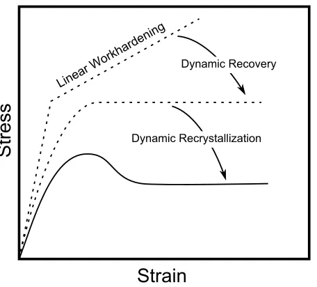
As the dislocation density increases during straining, nuclei are able to form during defor-mation [6]. Once recrystallization begins, dislocations in the material are eliminated. When the dislocation density gets low enough, recrystallization is halted until the strain increases the den-sity to a critical amount [6]. This increase, and subsequent decrease, in dislocations only occurs in materials with low- to medium-stacking fault energy that undergo deformation at temperatures near half of their melting points [1]. If a material with high-stacking fault energy undergoes the same heating and deformation process, the dislocations in the material are eliminated in pairs, which leads to steady state flow. This behavior in high-stacking fault materials is knows as “dy-namic recovery,” or DRV. A comparison of DRX and DRV is shown in Figure 2.1. The transition from linear hardworking to perfectly plastic flow occurs in the DRV region of the figure. Once the slope of the stress-strain curve begins to decline, the curve enters the DRX region.
cat-Figure 2.1: Dynamic recovery is evident by a non-linear stress-strain curve while dynamic re-crystallization results in a curve with a portion of the curve having a non-positive slope. Modified from [11].
egorized by the inverse number of coincident sites. For example, aΣ3boundary has 1/3of total
lattice sites are coincident.
boundary classifications. Brandon hypothesized that a boundary that deviates from the ideal CSL angle could be considered ideal if the misorientation was close to the ideal angle.
The Brandon criterion was developed based on the concept that CSL boundaries are able to be approximated as ideal CSLs as long as the boundary’s misorientation is within a specified number of degrees of the ideal CSL. For high densities of coincident sites (i.e., lowΣvalues), the degree of deviation from an ideal CSL is greater than for boundaries with higherΣvalues. Multiple variations of this criterion have been provided that are more conservative (i.e., Palumbo-Aust criterion), but for the purpose of this thesis, the Brandon criterion was selected. Using a criterion to simplify the possibly infinite misorientations into a discrete number of categories simplifies the calculations necessary to categorize grain boundaries. Brandon’s equation for the allowable angle of deviation,∆θmax, is as follows:
∆θmax =θ0Σ−1/2 (2.1)
whereθ0 is agreed to be 15◦ andΣis the CSL type (3 for aΣ3, etc.).
low-angle boundary will have significantly less boundary energy than a high-angle boundary but special high-angle boundaries exist with uncharacteristically low-boundary energy.
It has been shown [12, 15] that certain misorientations and grain boundary plane combina-tions result in lower grain boundary energy than would be expected for high-angle boundaries [9]. As shown in Figure 2.2, certain high-angle boundaries (those with misorientation angles of greater than 15◦) have a lower energy than others. These high-angle, low-energy boundaries occur when a boundary is said to havecoincidence, which is essentially when two grains have a high degree of fit (see Figure 2.3). A boundary has high coincidence when the density of over-lapping lattice sites is high. When a boundary has low coincidence, the lattice sites that do not overlap are terminated in a dislocation. The number of these dislocations and their placement determines the amount of energy associated with the boundary, as described by Read and Shock-ley’s dislocation model for low-angle and coincidence site lattice boundaries [9]. For general high-angle boundaries, the dislocation content is such that it is difficult to describe as an orderly array of dislocations.
Figure 2.3: A coincident boundary (left) occurs when the boundary coincides with the twinning plane. An non-coincident boundary (right) occurs when a boundary intersects the twinning plane at an angleθ. Modified from [17].
2.2 Strain and Stored Energy
Strain energy is the driving force for two processes in DRX, grain growth and recrystallization [8], and so it is prudent to include strain in any simulation that models DRX. In our simulations, strain energy is applied at a constant rate and stored in each tile in the simulational lattice. During DRX, two different methods take place to reduce both the stored energy and grain boundary energy in each tile, and therefore reduce the energy in the entire system.
Figure 2.4: Simulated equivalent of a stress-strain curve. The average stored energy in the sys-tem indicates which process is dominant: grain growth or recrystallization.
2.3 Recrystallization
Recrystallization is the formation of new grains, or nuclei. This thesis deals specifically with recrystallization that occursduring thermo-mechanical processing. It is important to recognize that recrystallization occurs both dynamically (DRX) and statically (SRX). The difference be-tween them is when the recrystallization occurs. SRX was observed prior to DRX and it was not until the 1960s that the difference between the two types of recrystallization was established [18]. Advancements in material characterization techniques were required in order to make the following distinctions: recrystallization during processing (which is considered DRX) and re-crystallizationafterprocessing (which is considered SRX).
Since the deviation in the observed nucleation rate, which was on the order of 1050 times larger than predicted, it is possible to state that the method of recrystallization during DRX is not the same as that which has been found in solidification and phase transformations.
Once DRX was identified, further studies were required to examine the behavior of recrystal-lization during DRX. The nuclei that form during DRX have been observed to be free of strain energy when they are initially formed [1, 19]. Proposed in 1949 by Cahn [20] using XRD and more recently supported by SEM results [21], an understanding has been established that nucle-ation is not the formnucle-ation of an entirely new grain, but rather a separnucle-ation of portions of existing grains. This separation occurs after a grain boundary becomes serrated and additional strain causes grain boundary shearing, which separates the serrated portion the and resulting rotation leads to the formation of a new grain (see Figure 2.5) [22, 23]. While this is one possible method of recrystallization, the exact mechanism of recrystallization is still unknown.
Experimental results show a number of preferences for nucleation during DRX. First, nuclei form “necklace” structures by nucleating along existing grain boundaries [23]. However, the most preferential nucleation location has been identified by Miura et al. as triple junctions, specifically at triple junctions with high-angle boundaries [8]. The nuclei that form at triple junctions have also been observed to formΣ3 boundaries with a neighboring grain [8].
2.4 Conditions of Dynamic Recrystallization
(a)Boundary corrugation accompanied by the evolution of subboundaries.
(b)Partial grain boundary shearing, lead-ing to the development of inhomoge-neous local strains.
(c)Bulging out of a serrated grain bound-ary and the evolution of strain induced subboundaries due to grain boundary shearing and/or grain rotation, leading to the formation of a new DRX grain.
Figure 2.5: A schematic modified model for the nucleation of a grain at a grain boundary (GB) [22].
The rate of DRX has been described by the Zener-Holloman parameter as follows:
Z = ˙ exp
−Q
RT
(2.2)
where ˙ is the strain rate, Q is the apparent activation energy for deformation, R is the gas constant, andT is the temperature. By this definition, a highZ value would describe conditions that are not favorable to DRX (high strain rate and low temperature), while one may be more likely to observe DRX under low Z conditions. The correlation of Z value and DRX behavior has been explored by Sakai and Jonas [6] with initial grain size. For example, a system with a lowZ value and a low initial grain size is likely to exhibit multiple peak behavior while a lowZ and a high initial grain size will be more likely to exhibit single peak behavior.
2.5 Kinetics of Dynamic Recrystallization
Besides exploring the mechanics of DRX, the rates of grain growth and nucleation are also of interest. One factor that affects the rate of recrystallization is grain size. Wahabi et al. [5] approached the kinetics of DRX by hypothesizing that the number of available nucleation sites directly relates to the kinetics of DRX. As nucleation occurs, the number of available sites de-creases; this point determines when the curve shown in Figure 2.4 returns to an upward slope. Experimentally, samples with smaller grain sizes have been observed to begin DRX earlier than samples with larger grains due to an abundance of grain boundaries on which nuclei can form while samples with larger grains experience a delay (during which stored energy,H, continues to increase) before beginning to nucleate [5].
of volume that has recrystallized) as:
dVt
dVex
= (1−Vt) (2.3)
where Vt is the transformed volume (volume of recrystallized grains) and Vex is the extended
volume (total volume of sample). Plotting the volume fraction of recrystallized material is useful for analyzing DRX as the rate of recrystallization and the time at which DRX starts can quantify the effect of various parameters on DRX.
The effect of initial grain size was explored further by Wahabi et al. [5] as a factor that affects the kinetics of DRX. Wahabiet al. demonstrated that microstructures with small initial average grain sizes recrystallized earlier than samples with larger initial average grain sizes. The reasoning behind this behavior was that samples with smaller grain sizes have a larger volume fraction of grain boundaries and therefore a higher number of available nucleation sites. This result supported the modified JMA equation for DRX kinetics, which includes an initial grain boundary term [6]:
X = 1−exp{−(K/D0)tn} (2.4)
whereXis the volume fraction of recrystallized material,Kandnare constants,D0is the initial
average grain size, andtis time. This equation shows that the rate of recrystallization is slower for larger initial grain size.
high-angle, low-energy boundaries would also experience a delay in the onset of recrystalliza-tion similar to the delay observed in large grain samples. Experimentarecrystalliza-tion has also shown [8] that while nucleation is preferred at triple junctions, triple junctions with twin boundaries (Σ3 boundaries) are much less preferred than triple junctions without twin boundaries.
2.6 Monte Carlo Simulation
Monte Carlo simulation uses random sampling to choose a site, then applies algorithms to reduce the energy in a system. Depending on the Hamiltonian associated with the system being simulated, the energy terms will continue to decrease each Monte Carlo step until steady state is attained. A “Monte Carlo step” is proportional to time. For any single step, a number of test sites are selected where the number of selections is equal to the number of discrete test sites present in the system.
First developed by Metropolis and Ulam [2], the Monte Carlo method was designed for ap-plications related to quantum physics. However, the apap-plications now stretch beyond those for which it was first developed [27, 28]. As stated in Section 1.2, Monte Carlo was found to be a suitable algorithm to simulate grain structure evolution [19]. Since that time, a number of modi-fied Monte Carlo methods have been developed [3]. The method used in this thesis deals with a Monte Carlo Potts Model, similar to what was used by Rollettet al. [29] and Peczak and Luton [30].
Tile shape also plays an important role in the lattice behavior. The lattice used is described as a triangular lattice with a hexagonal Wulff shape (Figure 2.7). As discussed by Rollett, a triangular lattice is suitable for 2D applications as its geometry does not inhibit grain growth [27].
Figure 2.7: Each hexagon represents an individual sample site. The varying colors represent the orientation of the particular tiles and similar orientations are grouped into grains and neighboring grains are separated by a grain boundary, noted here by a thick black line.
3 SIMULATION PROCEDURES
An earlier version of the code used for this work [31] was assembled using Visual Basic and Microsoft Excel. In order to make the code more universal (i.e., less dependent on a particular program and operating system) and to decrease computation time, the code was converted into ANSI C programming language.
Building an energy-based simulation requires energy equations to which minimization tech-niques can be applied. The inputs to the simulation consist of individual tiles that are grouped into grains based on similar orientations. An effort to reduce the overall system energy must then require the energy associated with individual tiles to be minimized.
While the boundary energy is important to simulate DRX, it is the value of the stored energy in the entire system that provides the most useful insights into the behavior of the simulation. Figure 2.4 is a plot of the average stored energy as a function of the Monte Carlo steps. A positive slope indicates that grain growth is the dominant process; when the curve has a negative slope, recrystallization is the dominant process and strain free grains are being created.
After a fixed number of Monte Carlo steps, the simulation totals the stored energy present in every tile. Dividing the total stored energy by the total number of tiles produces the average stored energy per tile (Eq. (3.1)):
Havg =
Htotal
n (3.1)
whereHavgis the average stored energy,Htotalis the sum of all the stored energy in all tiles, and
nis the total number of tiles.
3.1 Overview of Simulation Process
This research simulates DRX by performing a prescribed number of Monte Carlo steps. The program first counts the number of tiles present in the initial microstructure and that value is stored as the number of tiles that must be chosen at random each Monte Carlo step (MCS). While the algorithm for grain growth is allowed to occur every time a tile is selected, the recrystallization algorithm is only applied until a number of specified new grains are formed. Once a specific number (determined by the nucleation rate) of grains have been formed in a particular MCS, the recrystallization algorithm will be skipped until the next MCS. Also, at the beginning of each MCS, a fixed value is added to the stored energy value of each tile to simulate the continual deformation that occurs to produce DRX. The exact value that is added depends on the strain rate being simulated. For example, a smaller strain rate would add less stored energy per MCS than a larger strain rate. This process, illustrated schematically in Figure 3.1, repeats until the specified number of Monte Carlo steps have been performed.
3.2 Grain Boundary Classification
Figure 3.1: A flowchart showing the general concept of what occurs during the simulation. The dashed line represents what operations are performed each Monte Carlo step.
the energy of a boundary is based on the misorientation between two grains. The misorientation can be described as the transformation necessary to rotate the normal vector of one grain onto that of its neighbor. Before the misorientation can be calculated, an orientation matrix for each grain must be determined as:
gx =
g11 g12 g13
g21 g22 g23
g31 g32 g33
wheregx is the orientation matrix, the subscriptxdenotes a specific grain, and each element of
the matrix is described as:
g11 = cos(φ1) cos(φ1)−sin(φ1) sin(φ2) cos(Φ)
g12 = sin(φ1) cos(φ2)−cos(φ1) sin(φ2) cos(Φ)
g13 = sin(φ2) sin(Φ)
g21 =−cos(φ1) sin(φ2)−sin(φ1) cos(φ2) cos(Φ)
g22 =−sin(φ1) sin(φ2)−cos(φ1) cos(φ2) cos(Φ)
g23 = cos(φ2) sin(Φ)
g31 = sin(φ1) sin(Φ)
g32 =−cos(φ1) sin(Φ)
g33 = cos(Φ)
whereφ1,φ2, andΦare the Euler angles for a grain and used to describe the deviation from the
coordinate system used during EBSD scanning.
For the purpose of simplicity, only two grains will be considered during these calculations, grain A and grain B. Therefore, each grain will have an orientation matrix: gAandgB. After an
orientation matrix for each grain has been developed, the misorientation between grains A and B,∆gAB, can be determined as:
Once the misorientation matrix (∆gAB) has been determined, it is multiplied by the 24 possible
rotations for a cubic crystal structure to determine the minimum rotation necessary to rotate grain A onto grain B. The minimum rotation angle,θAB, is determined by:
θAB = cos−1
3 P i=1
aii−1
2 (3.4)
where aii represents the diagonal elements of ∆gAB ·R with R being one of the 24 possible
rotation matrices (each rotation matrix represents rotation about a different rotation axis). In short, the rotation matrix that results in the largest trace is the rotation operation that rotates grain A to match the orientation of grain B with the smallest angle of rotation. The result of multiplying∆gAB by the rotation matrix, which results in the lowest angle of rotation,Rmin, is
then compared to the 24 possible rotation matrices using the equation:
∆θ = (∆gAB·Rmin)·A−CSL1 (3.5)
where∆θ is the angular deviation of the misorientation from an ideal CSL boundary andACSL
is the matrix used to describe each ideal CSL boundary. The∆θmatrix that results in the largest trace (i.e., the smallest angle) then determines the CSL to which the boundary between grains A and B is closest. A final step in the boundary characterization process is to compare the resulting angle from ∆θmin to the maximum deviation specified by the Brandon criterion for
energy of a general boundary, which was obtained experimentally. For example, the energy of a general boundary in 304 stainless steel is 835 mJ·m−2 and the energy of a coherent twin boundary (Σ3) is 19 mJ·m−2, or 5% of the energy of a general boundary [17]. Therefore, the
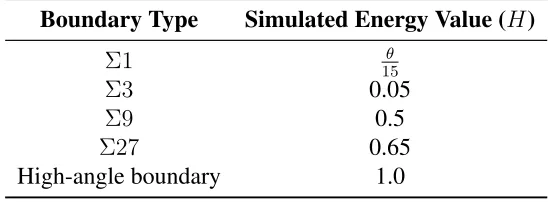
simulation assigns an energy of 1.0 (or 100%) to a boundary found to be general and 0.05 (or 5%) to aΣ3boundary. OtherΣboundaries were assigned energies between 0.05 and 0.65 as the particular energies of these boundaries were not the primary focus of this work. A summary of the grain boundary energies used for this work can be found in Table 3.1. The energy value for Σ1boundaries was assigned by approximating the energy equation
Table 3.1:A list of the grain boundaries that are taken into account by the simulation and their assigned energy values.
Boundary Type Simulated Energy Value (H)
Σ1 15θ
Σ3 0.05
Σ9 0.5
Σ27 0.65
High-angle boundary 1.0
(a)J0 (b)J1 (c)J2 (d)J3
Figure 3.2: (a) Shows a triple junction with no special boundaries present, (b) with a single spe-cial boundary, (c) with two spespe-cial boundaries, and (d) with three spespe-cial boundaries.
In order to validate the results of the simulation, the special boundary fractions of experi-mentally obtained EBSD scans being reported by the simulation were compared to the fractions reported by commercially obtained software TSL OIM Analysis 5. The results from this com-parison resulted in a restriction being placed on the minimum misorientation angle between two tiles in order to determine if a boundary exists or not. This has the largest effect on the num-ber ofΣ1 boundaries reported by the output files of the simulation and the TSL software. This minimum misorientation requirement prevents an unusually large number ofΣ1boundaries from being reported and shown on the figures produced by the TSL software. For the purpose of this simulation, tiles with a misorientation of less than four degrees are considered to be the same grain and therefore not be separated by a boundary.
3.3 Dynamic Recrystallization
For a purely energy driven simulation, the decision of whether or not to nucleate a grain depends on the current energy at a test site and what the energy would be should a nucleus form. The energy difference between the proposed and existing tiles must be less than the energy required to form a new grain in order for nucleation to occur. The following relationship was used as a decision-making criteria of whether or not to nucleate a new grain:
Nucleate if:∆γ+ ∆H+Ef orm≤0 (3.6)
where ∆γ was the change in grain boundary energy, ∆H is the change in stored energy, and Ef orm is the energy required form a new grain. The value of Ef orm was considered a variable
and can be altered in order to allow future accommodation of various materials. Physically, Ef orm corresponds to the energy required for a portion of an atomic lattice to break its bonds
with a parent grain and reorient to a new grain. It was assumed that each material may require a different amount of stored energy that is required to cause recrystallization.
(a) (b)
Figure 3.3: During simulated recrystallization, a random tile and two neighboring tiles are cho-sen and tested to see if it is energetically favorable to nucleate. Should the conditions be favorable to form a nucleus, a strain-free grain is formed and the stored energy is set to zero. (a) shows the initial microstructure and (b) shows the microstructure af-ter a nucleus is formed. Each color represents a separate grain. The numbers within the tiles represent the stored energy.
The portion of this thesis that deals with the study of DRX kinetics requires information that tracks the onset and progression of recrystallization. While subsequent recrystallization cycles may differ between samples with high special boundary fractions and those with low fractions, it is the initial recrystallization cycle that is of interest. After the initial cycle, the special boundary fraction of both the high-fraction and low-fraction samples is similar. This means that the effect of special boundaries on DRX kinetics will be most evident during the first cycle. The equation to calculate the percent of grains that have been recrystallized is:
%recrystallized=
nrx
n (3.7)
wherenrx is the number of tiles in recrystallized grains and nis the total number of tiles in the
sample.
3.4 Grain Growth Algorithms
Unlike the kinetics of recrystallization, grain growth kinetics do not depend solely on the formation energy. Should a test site be found where the change in energy between the initial situation and a situation where grain growth occurs, only a certain percentage of favorable grain growth operations are retained. Whether a favorable grain orientation reassignment is retained or not depends on the following equation:
P(∆E) =
not retained if∆E >0
retained if∆E ≤1& −κ2 ≥1
(3.8)
where is an integer selected at the start of the simulation as part of the test parameters and κ is a random integer chosen between zero and. With regards to the physical interpretation of: larger values means slower grain growth.
The energy calculations of grain growth do not rely solely on the values of boundary energy, but also on the value of stored energy present in the grain. For example, nucleated grains have their stored energy reset to zero. A grain with little to no strain energy will be much more likely to grow than a heavily strained grain. However, as a grain grows, it will be affected by the strain of the neighboring grains. Should a grain growth operation be retained, the chosen tile next to the sample site is assigned the same orientation as the sample tile. Strain energy in the adjacent tile is averaged between its original value and the value of the sample tile. Figure 3.4 shows how the grain growth algorithm averages the stored energy between the two grains present in random location chosen during the Monte Carlo step.
(a) (b)
Figure 3.4: Schematic of (a) Two neighboring grains (denoted by red and blue colors) with dif-fering stored energy values. (b) The left grain grows by a single tile (hexagon) and the stored energy of that tile is an average of the two tiles chosen as a possible grain growth site.
simplify calculations, and rather than explicitly calculating the radius of curvature of two grains at a sample site, the number of tiles present in each grain were compared and the grain with more tiles was assumed to have a larger radius. The energy associated with curvature,Ec, is described
as:
Ec=
nA−nB
max{nA, nB}
(3.9)
wherenA is the number of tiles in the grain associated with the initially selected tile andnB is
the number of tiles in the grain associated with the neighboring tile. Should nA be larger, the
chance of grain growth is increased due to the added energy associated with curvature. However, the value of Ec would be negative if the value of nB was larger than nA and therefore would
hinder grain growth at that particular site. The equation for curvature limits the value of Ec
would be more resistant to the effects of curvature. Table 3.2 shows the reduction of the effect of curvature based on boundary type. Overall, a balance had to be achieved between the effect of grains that have already grown substantially against the effect of a newly nucleated grain that has a substantially smaller radius of curvature but is strain-free in order to ensure that newly nucleated grains “survived” in the simulation.
Table 3.2:List of grain curvature coefficients. HigherΣboundaries are more mobile and there-fore the effect of curvature would have a greater effect.
EcCoefficient
Σ1 0.1
Σ3 0.1
Σ9 0.2
Σ27 0.3
4 RESULTS AND DISCUSSION
4.1 Initial Microstructure
Two initial microstructures were obtained from EBSD scans of separate samples of 316L stainless steel and are shown in Figure 4.1. One of the samples underwent a single grain bound-ary engineering process while the other sample underwent multiple grain boundbound-ary engineering (GBE) processes. During GBE, the special boundary fraction significantly increases, as shown in Table 4.1. Each GBE process a material undergoes further increases the fraction of special boundaries. The “low-fraction” and “high-fraction” samples have been labeled according to their respective initial special boundary fraction. The initial average grain size for each sample is rel-evant as significantly different average grain sizes can affect the kinetics of DRX. The samples chosen for this research deviate by only approximately 11 tiles per grain (the low-fraction sample is approximately 13% smaller than the high-fraction). It has been determined that the average grain size between the samples is similar enough to reduce the effect of grain size, allowing the effect of special boundies to be more pronounced.
Table 4.1: Special boundary information for starting microstructure.
Special Boundary Σ3 Fraction Initial Avg. Fraction (% by length) Grain Size
(% by length) (# of tiles/grain)
Low-Fraction 69.8 56.5 76.06
(a)Low-Fraction (b)High-Fraction
Figure 4.1: Experimentally obtained EBSD scan of 316L Stainless Steel for (a) a sample that has undergone a single GBE cycle and (b) a sample that has undergone three GBE cycles. Solid colors represent grain orientation while thin lines represent grain boundaries. Black grain boundaries are general boundaries while red areΣ3boundaries.
4.2 Simulating Experimental Trends in DRX
During simulation, the number of original grains present at every MCS were compared to the initial number of original grains. This provides a method of tracking the kinetics of recrystal-lization and allows microstructures showing various stages of recrystalrecrystal-lization to be shown with the average stored energy as a function of time. As shown in Figure 4.4, the majority of the first recrystallization cycle occurs during the first peak. This matches expected behavior where por-tions of a stress-strain curve with a positive slope correspond to grain growth dominated behavior while negative sloped portions are where recrystallization occur.
Figure 4.5 shows evidence that the trends observed in experiments are also found in the sim-ulation. The characteristic DRX behavior of stress-strain curves transitioning from single-peak to multi-peak behavior with decreasing strain rate and/or increasing temperature is replicated reasonably well. Due to the ability to model the general behavior of DRX, the details behind the mechanisms of DRX and the related changes to microstructure can be observed, compared to experimental results, identified, and then characterized in a way to allow the microstructural changes to be predicted.
The data from each simulation allowed the extraction of the peak average stored energy and allowed analysis of the magnitude of the peak. Figure 4.6 shows the maximum peak and the strain rate at which it occurred. The highest peak values correspond to the largest strain rates. This is most likely due to the fact that higher strain rates increase the stored energy faster than can be initially removed by grain growth and recrystallization. The higher strain rate also increases the difference between the high and low-temperature peaks.
4.3 Temperature Effects
(a)Low-Fraction
(b)High-Fraction
(a)Low-fraction
(b)High-fraction
to remove the strain energy efficiently with even the lowest grain growth and nucleation rates. However, at higher strain rates, the higher grain growth and nucleation rates that occur during the high temperature simulation are able to achieve a steady state average stored energy more quickly.
Figure 4.5 shows the effect of temperature for the low and high-fraction samples at various strain rates. In both samples, the low-temperature peaks are higher and shifted to the right. A shift of the peak to the right implies that the recrystallization portion of the simulation is delayed. This is due to the lower nucleation rates. At lower temperature, nucleation attempts occur less frequently and the stored energy in the simulation must reach a sufficient level such that every nucleation attempt results in a successful nucleation. At higher temperatures, the nucleation rate is higher and therefore a favorable nucleation location may be found earlier in the simulation.
4.4 Effect of Special Boundary Fraction
requires that the energy of the nucleus being formed be less than the energy previously present at the nucleation site. The presence of even a single special boundary reduces the desirability of a nucleation site a significant amount. In order to nucleate at a site with a special boundary, the stored energy removed by the nucleation of a strain-free grain must offset the energy gained by forming (most likely) a nucleus enclosed in general boundaries.
(a)Low-fraction (b)High-fraction
Figure 4.7: Comparing rates of recrystallization for isotropic and anisotropic simulations. Both the low and high-fraction samples showed that recrystallization was delayed for anisotropic simulations when compared to isotropic runs. The delay in recrystal-lization is more pronounced for the high-fraction sample.
While it may seem to be a result that runs counter to what is expected (since special boundary fraction was expected to result in different behavior), the difference in special boundary fraction is removed after the first recrystallization cycle. Once the special boundary fractions become similar in the two samples, it stands to reason that their average stored energy values between the two samples would be similar. As the initial microstructure is replaced by grains of random orientation, the special boundary fraction decreases in all situations to a similar percentage.
Figure 4.8: Plot of low and high-fraction samples at the same temperature and strain rate. Note that the energy peaks for the high-fraction samples are lower and shifted to the right when compared to energy peaks for the low-fraction sample. Physically, this would correspond to an earlier onset of DRX.
have lower stress values and the peak stress value were shifted to the right. It was concluded that this was due to smaller grain sizes providing more nucleation sites [5]. Conversely, the delay in the maximum peak value for larger grain sizes corresponded to a delay in the onset of DRX and was hypothesized to occur due to the lower number of nucleation sites. From these observations, it appears that the initial special boundary fraction alters the effective initial grain size: higher initial special boundary fractions effectively increases the initial grain size.
(a) (b)
Figure 4.9: Comparing special boundary fraction to (a) the maximum average stored energy as well as (b) the time required to reach the maximum average stored energy. The data shows that there may be a similar correlation between the effect of special bound-aries and the effect of initial grain size: higher special boundary fractions have the potential to have a similar effect as larger initial grain sizes.
nucleus forms aΣ3boundary with a neighboring grain, and assuming all boundaries are of equal length, the maximum possible special boundary fraction would be 30%. However, since the spe-cial boundary fraction is calculated by length, and not all boundaries are of equal length, a steady state fraction of special boundaries around 22% seems reasonable after recrystallization.
The reason for this direct relationship between initial special boundary fraction and the onset of recrystallization is due to the relationship between the low energy of special boundaries and the effect they have on decreasing the desirability of forming nuclei on them. Since nucleation occurs along grain boundaries, lower energy at these sites mean that it is more efficient for the system to continue to attempt grain growth rather than nucleation until the stored energy reaches a point where forming boundaries around a strain-free grain is more favorable.
The reason for the change in the special boundary fraction can be attributed to the introduc-tion of energetically preferable boundaries. By forcing low-energy boundaries to form during recrystallization, the number of preferred nucleation sites in the system is decreased. In order for a nuclei to form on a non-preferred site, the strain energy within a grain must increase to the point at which the grain boundary energy becomes irrelevant. This means that the simulation must progress longer to add the necessary strain and therefore the rate at which the special bound-ary fraction decreases is diminished. The steady state value for the special boundbound-ary fraction is also increased due to the presence of energetically favorable boundaries.
4.5 Nucleation Location and Available Nucleation Sites
(a)15%Σ3 forced (b)50%Σ3 forced
(c)75%Σ3 forced (d)100%Σ3 forced
information for the first cycle of each sample before the variations in special boundary fraction between the two samples are removed by complete recrystallization.
Figure 4.14: Comparison of available triple junction sites to the actual location at which nucle-ation occurs. The shaded area on the left plot denotes the portion of the simulnucle-ation dominated by grain growth. Solid bars on right graph denote the fraction of nuclei that formed for each boundary type. Lighter bars denote initial fraction of avail-able nucleation sites of each type at 4,000 MCS. Higher J-value sites nucleate less favorably.
5 CONCLUSIONS
5.1 Implications
In conclusion, the simulation developed for this work is able to replicate several important trends observed in experimental DRX research. Previous work showed the importance of temper-ature, strain rate, and observation of nucleation occurring primarily on grain boundaries [8, 11]. This work was able to simulate the effect of temperature and strain rate and successfully show that increasing temperature and decreasing strain rate lower the average stored energy and plotted curves transition from single-peak to multi-peak. This work also showed that nucleation occurred at grain boundaries in necklace structures.
A step towards bridging the gap between experimental and simulational results was achieved by accepting experimental EBSD scans as initial microstructure. From these scans, it was possi-ble to calculate grain boundary energy based on grain misorientation to allow for simulation of anisotropic boundary energy. Over the course of the simulation, it was possible to track nucle-ation locnucle-ation and separate into triple junction vs. non-triple junction locnucle-ations and differentiate between four types of triple junctions (J0, J1, J2, and J3).
prefer-ential nucleation locations (as shown experimentally [8]). Specifically, nucleation is favored at lower J-value triple junctions (i.e., J0, J1).
5.2 Future Work
REFERENCES
[1] R. D. Doherty, D. A. Hughes, F. J. Humphreys, J. J. Jonas, D. J. Jensen, M. E. Kassner, W. E. King, T. R. McNelley, H. J. McQueen, and A. D. Rollett, “Current Issues in Recrys-tallization: a Review,” Mat. Sci. Eng. A - Struct.,238[2] 219–274 (1997).
[2] N. Metropolis and S. Ulam, “The Monte Carlo Method,” J. Am. Stat. Assoc., 44 [247] 335–341 (2002).
[3] K. G. F. Janssens, D. Raabe, E. Kozeschnik, M. A. Miodownik, and B. Nestler, “Monte Carlo Potts Model”; pp. 57–84 in Computational Materials Engineering: An Introduction to Microstructure Evolution, Elsevier Academic Press, 30 Corporate Drive, Suite 400, Burlington, MA 01803, USA, 2007.
[4] M. E. Wahabi, J. M. Cabrera, and J. M. Prado, “Hot Working of Two AISI 304 Steels: a Comparative Study,” Mat. Sci. Eng. A - Struct.,343[1-2] 116–125 (2003).
[5] M. E. Wahabi, L. Gavard, F. Montheillet, J. M. Cabrera, and J. M. Prado, “Effect of Initial Grain Size on Dynamic Recrystallization in High Purity Austenitic Stainless Steels,” Acta. Mater.,53[17] 4605–4612 (2005).
[6] T. Sakai and J. J. Jonas, “Overview No. 35: Dynamic Recrystallization: Mechanical and Microstructural Considerations,” Acta. Metall.,32[2] 189–209 (1984).
[7] R. Sandstrom and R. Lagneborg, “Controlling Factor for Dynamic Recrystallization,”
[8] H. Miura, T. Sakai, H. Hamaji, and J. J. Jonas, “Preferential Nucleation of Dynamic Re-crystallization at Triple Junctions,” Scripta Mater.,50[1] 65–69 (2004).
[9] W. T. Read and W. Shockley, “Dislocation Models of Crystal Grain Boundaries,” Phys. Rev.,78[3] 275–289 (1950).
[10] D. L. Olmsted, S. M. Foiles, and E. A. Holm, “Survey of Computed Grain Boundary Properties in Face-Centered Cubic Metals: I. Grain Boundary Energy,” Acta. Mater., 57
[13] 3694–3703 (2009).
[11] R. A. Petkovic, M. J. Luton, and J. J. Jonas, “Recovery and Recrystallization of Carbon-Steel Between Intervals of Hot Working,” Can. Metall. Quart.,14[2] 137–145 (1975).
[12] D. G. Brandon, “Structure of High-Angle Grain Boundaries,” Acta. Metall.,14[11] 1479– 1484 (1966).
[13] W. T. Read and W. Shockley, “Quantitative Predictions from Dislocation Models of Crystal Grain Boundaries,” Phys. Rev.,75[4] 692–692 (1949).
[14] W. Burgers, C. Dunn, F. Lionetti, A. Shaler, and L. Jaffe, “The Effect of Orientation Dif-ference on Grain Boundary Energies - Discussion,” T. Am. I. Min. Met. Eng., 185 [11] 860–862 (1949).
[15] D. G. Brandon, B. Ralph, S. Ranganathan, and M. S. Wald, “A Field Ion Microscope Study of Atomic Configuration at Grain Boundaries,” Acta. Metall.,12[7] 813–821 (1964).
[16] A. F. Gourgues, “Electron Backscatter Diffraction and Cracking,” Mater. Sci. Technol.,18
[17] F. J. Humphreys and M. Hatherly, “The Structure and Energy of Grain Boundaries”; pp. 47–108 in Recrystallization and Related Annealing Phenomena, Elsevier Science Ltd., The Boulevard, Langford Lane, Kidlington, Oxford OX5 1GB, UK, 1995.
[18] H. J. McQueen, “Development of Dynamic Recrystallization Theory,” Mat. Sci. Eng. A -Struct.,387203–208 (2004).
[19] F. J. Humphreys and M. Hatherly, “Recovery and Recrystallization During and After Hot Deformation”; pp. 363–392 in Recrystallization and Related Annealing Phenomena, El-sevier Science Ltd., The Boulevard, Langford Lane, Kidlington, Oxford OX5 1GB, UK, 1995.
[20] R. W. Cahn, “Recrystallization of Single Crystals After Plastic Bending,” J. I. Met.,76[2] 121–143 (1949).
[21] M. Jafari and A. Najafizadeh, “Correlation Between Zener-Hollomon Parameter and Neck-lace DRX During Hot Deformation of 316 stainless steel,” Mat. Sci. Eng. A - Struct., 504
[1-2] 16–25 (2009).
[22] A. Belyakov, H. Miura, and T. Sakai, “Dynamic Recrystallization Under Warm Deforma-tion of a 304 Type Austenitic Stainless Steel,”Mat. Sci. Eng. A - Struct.,255[1 - 2] 139–147 (1998).
[23] D. Ponge and G. Gottstein, “Necklace Formation During Dynamic Recrystallization: Mech-anisms and Impact on Flow Behavior,” Acta. Mater.,46[1] 69–80 (1998).
[25] A. Dehghan-Manshadi and P. D. H. M. R. Barnett, “Characterization of Austenite Dynamic Recrystallization under Different Z Parameters in a Microalloyed Steel,” Mat. Sci. Eng. A -Struct.,485[4] 664–672 (2008).
[26] C. W. Price, “Use of Kolmogorov-Johnson-Mehl-Avrami Kinetics in Recrystallization of Metals and Crystallization of Metallic Glasses,” Acta. Metall. Mater., 38 [5] 727–738 (1990).
[27] A. D. Rollett, “Overview of Modeling and Simulation of Recrystallization,” Prog. Mater. Sci.,42[1-4] 79–99 (1997).
[28] N. Xiao, D. Li, and Y. Li, “Numerical Investigation of Deformation-Induced Transforma-tion in Fe-C alloy Using a Q-state Potts Monte Carlo Model”; pp. S169–S176 TMS 2009 138th Annual Meeting & Exhibition: Supplemental Proceedings, Vol. 2.
[29] A. Rollett, M. Luton, and D. Srolovitz, “Microstructural Simulation of Dynamic Recrystal-lization,” Acta. Metall.,40[1] 43 (1992).
[30] P. Peczak and M. Luton, “A Monte Carlo Study of the Influence of Dynamic Recovery on Dynamic Recrystallization,” Acta. Metall.,41[1] 59 (1993).