Composites for Biomedical Applications

(1)

Doctoral School in Materials Engineering – XXII cycle

Composites for Biomedical Applications

Fabio Zomer

Fabio Zomer Volpato

Volpato

(2)

(3)

Doctoral School in Materials Engineering – XXII cycle

Composites for Biomedical Applications

Fabio Zomer

Fabio Zomer Volpato

Volpato

Advisor:

Prof. Claudio Migliaresi

(4)

(5)

Contents

1 INTRODUCTION AND OBJECTIVES 15

1.1 Introduction . . . 15

1.2 Objectives . . . 17

1.2.1 Specific Objectives . . . 17

2 STATE OF THE ART 19 2.1 Tissue Engineering . . . 19

2.2 Scaﬀolds in Tissue Engineering . . . 21

2.3 Polymers in Tissue Engineering . . . 21

2.3.1 Natural polymers . . . 22

2.3.2 Synthetic polymers . . . 23

2.4 Composites in Tissue Engineering . . . 23

2.5 Surface Features . . . 24

2.5.1 Micro patterning . . . 25

2.5.2 Nano patterning . . . 25

2.6 Carbon Nanotubes . . . 26

2.6.1 Single-walled carbon nanotubes . . . 27

2.6.2 Multi-walled carbon nanotubes . . . 28

2.6.3 Production technique . . . 29

2.6.3.1 Chemical Vapor Deposition (CVD) . . . 29

2.6.3.2 Arc-Discharge . . . 30

2.6.3.3 Laser ablation . . . 30

(6)

2.6.4 Properties . . . 30

2.6.4.1 Mechanical properties . . . 30

2.6.4.2 Electrical properties . . . 31

2.6.4.3 Optical properties . . . 31

2.6.5 Carbon nanotubes in tissue engineering . . . 32

2.6.5.1 Carbon nanotubes biocompatibility . . . 33

2.7 Electrospinning Technique . . . 34

2.7.1 Electrospinning theory . . . 37

2.7.1.1 Droplet generation . . . 37

2.7.1.2 Taylor’s cone formation . . . 38

2.7.1.3 Launching of the jet . . . 38

2.7.1.4 Elongation of straight segment . . . 39

2.7.1.5 Whipping instability region . . . 40

2.7.1.6 Solidification into nanofiber . . . 41

2.7.2 Main parameters that influence fiber morphology 41 2.7.2.1 Electrical field . . . 41

2.7.2.2 Polymer concentration . . . 42

2.7.2.3 Flow rate . . . 42

2.7.2.4 Working distance . . . 42

2.7.3 Electrospinning for biomedical applications . . . . 43

3 MATERIALS AND METHODS 45 3.1 Polyamide 6 - PA6 . . . 45

3.2 Functionalized Multi-Walled Carbon Nanotubes . . . 46

3.3 Fabrication Technique . . . 46

3.4 Characterization Methods . . . 49

3.4.1 Carbon nanotubes analyses . . . 49

3.4.1.1 Transmission electron microscopy - TEM 49 3.4.1.2 X-Ray photoelectron spectroscopy - XPS 49 3.4.2 Nanofiber morphology . . . 50

(7)

CONTENTS 3

3.4.2.2 Transmission electron microscopy - TEM 50

3.4.2.3 Atomic force microscopy - AFM . . . 51

3.4.3 Thermal analysis . . . 51

3.4.3.1 Diﬀerential scanning calorimetry - DSC 51 3.4.4 Mechanical analysis . . . 52

3.4.4.1 Tensile analysis . . . 52

3.5 Biological Evaluation . . . 52

3.5.1 Protein adsorption analyses . . . 53

3.5.1.1 Protein adsorption . . . 53

3.5.1.2 Electrophoresis . . . 54

3.5.2 Cell seeding and culture . . . 54

3.5.3 Cell proliferation . . . 55

3.5.4 Cell viability . . . 56

3.5.5 Cell morphology . . . 57

3.6 Statistical Analysis . . . 57

4 RESULTS AND DISCUSSION 59 4.1 Carbon Nanotubes Analysis . . . 59

4.2 Nanofiber Production and Morphology . . . 61

4.3 Thermal Analysis . . . 66

4.4 Mechanical Analysis . . . 71

4.5 Biological Analysis . . . 74

4.5.1 Protein analyses . . . 74

4.5.2 Proliferation analysis . . . 77

4.5.3 Cell viability . . . 80

4.5.4 Cell morphology . . . 86

5 CONCLUSIONS 95

6 FUTURE INVESTIGATIONS 99

(8)

(9)

List of Figures

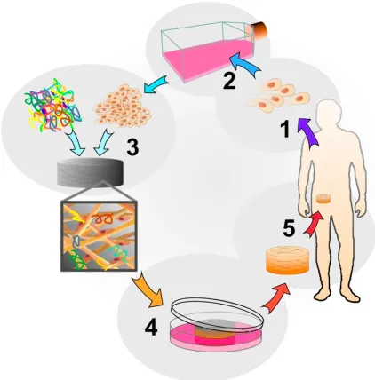
2.1 Tissue Engineering approach representation. (http://biomed .brown.edu). . . 20 2.2 Molecular structures of a single-walled carbon nanotube

(SWCNT) and of a multi-walled carbon nanotube (MWCNT). (http://www-ibmc.u-strasbg.fr/). . . 27 2.3 TEM image of a single-walled carbon nanotube. (http://

www.electroiq.com). . . 28 2.4 TEM image of a multi-walled carbon nanotube. (http://

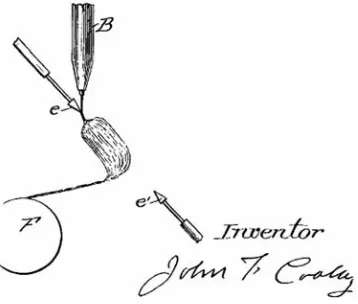
endomoribu.shinshu-u.ac.jp/). . . 29 2.5 Electrospinning diagram drawn by Cooley in 1902, where

A is a solution of polymer (e.g., collodion or cellulose ni-trate in ether or acetone) delivered into the high-voltage direct current (DC) electric field via tube B to form elec-trospun nanofibers collected on a drum F. [1] . . . 35 2.6 Number of article publications in the past years relevant

to electrospinning. [2] . . . 36 2.7 Most common electrospinning apparatus. [3] . . . 37 2.8 a) Optical image of the Taylor’s cone and tapering linear

segment of a jet emanating from a microfabricated silicon tip. (b) Diagram of diﬀerent geometries of Taylor’s cone obtained in practice. [4] . . . 39

(10)

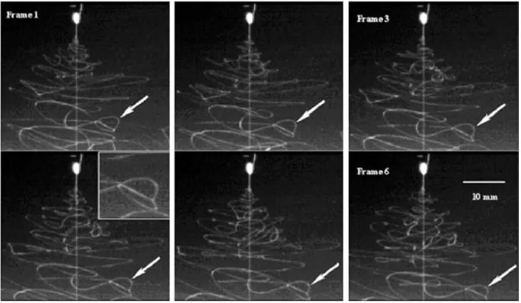
2.9 Trajectories of the jet in the whipping instability region during the electrospinning of PCL in 15 wt% acetone so-lution (applied voltage is 5 kV and gap distance is 14 cm). [5] . . . 40

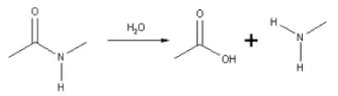
3.1 Hydrolytic degradation of amide groups in the polyamide backbone. . . 46 3.2 TEM micrography of the supplied MWCNTs. Source:

Cheap Tubes. . . 47 3.3 Electrospinning safety box, S1 shows the static system and

S2 the dynamic system. . . 49 3.4 Apparatus control box. . . 50

4.1 TEM image of the supplied multi-walled carbon nanotubes. 60

4.2 XPS survey spectra of the supplied MWCNTs. . . 60 4.3 C1s fitting of XPS survey spectra. . . 61 4.4 O1s fitting of XPS survey spectra. . . 61 4.5 The influence of applied voltage on the fiber alignment of

PA6, when the target tangential speed is 3.33 m/s. (A) 20 kV, (B) 15 kV and (C) 5 kV. . . 62 4.6 Random PA6 (A) and aligned PA6 (B) produced networks. 63 4.7 Random PA6/CNT (A) and aligned PA6/CNT (B)

pro-duced networks. . . 63 4.8 Histogram representing the random and aligned PA6 fiber

diameter distribution. . . 64 4.9 Histogram representing the random and aligned PA6/CNT

fiber diameter distribution. . . 65 4.10 Transmission electron micrography of PA6/CNT

(11)

LIST OF FIGURES 7

4.11 AFM images depicting the surface topography of the (A) PA6 and (B) PA6/CNT fibers. . . 66 4.12 Fiber profile acquired from the AFM images, (A) PA6 and

(B) PA6/CNT. . . 66 4.13 Partial thermogram depicting the water adsorption region. 68 4.14 First scan partial thermogram depicting the melting region. 69 4.15 Partial thermogram depicting the crystallization region. . 70 4.16 Second scan partial thermogram depicting the melting

re-gion. . . 71 4.17 PE/MWCNT NHSK structure produced by solution

crys-tallization of PE on MWCNTs at 103 °C in p-xylene for 30 min. (a) SEM image of MWCNTs decorated by disc-shaped PE single crystals. (b) TEM image of the PE/MWCNT NHSK structure. (c) Schematic representation of the PE/CNT NHSK structure. PE forms lamellar single crystals on CNT surface with polymer chains parallel to the CNT axis. [6] . . . 72 4.18 Typical stress-strain curves of orthogonal and parallel

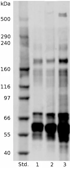
re-garding the spinning direction. . . 73 4.19 Protein adsorption after treatment with 0.1% SDS, where

(Std.) HImark Standard, (1) TCP control, (2) Random PA6, (3) Aligned PA6, (4) Random PA6/CNT and (5) Aligned PA6/CNT. ImperialT M _{stain. . . .} ₇₅

4.20 Protein adsorption after treatment with 0.1% SDS, where (Std.) HImark Standard, (1) TCP control, (2) MG63 medium and (3) inactive FBS. ProteoSilverT M _{stain. . .} ₇₅

(12)

4.22 Alamar Blue proliferation assay of the tested networks cul-tured with MG63 cell line. * p< 0.0001 and ** p<0.5. . 78 4.23 Alamar Blue proliferation assay of the tested networks

cul-tured with MRC5 cell line. * p< 0.0001 and ** p<0.5. . 79 4.24 Fibroblasts surrounded by (collagen fibrils) a scaﬀold. . . 80 4.25 Cell viability analysis of MG63 cell culture on diﬀerent

sur-faces for 3 days. (A) Random PA6, (B) Aligned PA6, (C) Random PA6/CNT and (D) Aligned PA6/CNT networks. 81 4.26 Cell viability analysis of MG63 cell culture on diﬀerent

sur-faces for 7 days. (A) Random PA6, (B) Aligned PA6, (C) Random PA6/CNT and (D) Aligned PA6/CNT networks. 82 4.27 Cell viability analysis of MG63 cell culture on diﬀerent

surfaces for 14 days. (A) Random PA6, (B) Aligned PA6, (C) Random PA6/CNT and (D) Aligned PA6/CNT net-works. . . 83 4.28 Cell viability analysis of MRC5 cell culture on diﬀerent

surfaces for 14 days. (A) Random PA6, (B) Aligned PA6, (C) Random PA6/CNT and (D) Aligned PA6/CNT net-works. . . 86 4.31 SEM images of MG63 cell culture on diﬀerent surfaces for

(13)

LIST OF FIGURES 9

4.32 SEM images of MG63 cell culture on diﬀerent surfaces for 7 days. (A) Random PA6, (B) Aligned PA6, (C) Random PA6/CNT and (D) Aligned PA6/CNT networks. . . 88 4.33 SEM images of MG63 cell culture on diﬀerent surfaces for

14 days. (A) Random PA6, (B) Aligned PA6, (C) Random PA6/CNT and (D) Aligned PA6/CNT networks. . . 89 4.34 SEM images of MRC5 cell culture on diﬀerent surfaces for

3 days. (A) Random PA6, (B) Aligned PA6, (C) Random PA6/CNT and (D) Aligned PA6/CNT networks. . . 90 4.35 SEM images of MRC5 cell culture on diﬀerent surfaces for

7 days. (A) Random PA6, (B) Aligned PA6, (C) Random PA6/CNT and (D) Aligned PA6/CNT network. . . 91 4.36 SEM images of MRC5 cell culture on diﬀerent surfaces for

14 days. (A) Random PA6, (B) Aligned PA6, (C) Random PA6/CNT and (D) Aligned PA6/CNT networks. . . 92 4.37 Micrography depicting the upper cell layer alignment after

14 days of culture with MG63. Aligned (A) PA6 and (B) PA6/CNT network. . . 93 4.38 High magnification SEM micrography depicting the

cel-lular ingrowth on the scaﬀolds surface after 14 days of culture with MG63. Aligned (A) PA6 and (B) PA6/CNT network. . . 93 4.39 High magnification SEM micrography illustrating the

cel-lular ingrowth on the scaﬀolds surface after 14 days of culture with MRC5. (A) Aligned PA6 and (B) Random PA6/CNT network. . . 94 4.40 High magnification SEM micrography depicting the

(14)

(15)

List of Tables

3.1 Manufactures datasheet for the functionalized 30-50nm MWCNTs. . . 47 3.2 Electrospinning parameters used in the project. . . 48

4.1 Quantitative analysis of the C1s and O1s peaks. . . 61 4.2 Most adapted parameters applied for the networks

pro-duction. . . 62 4.3 Thermal analysis results representing the pure PA6 and

composite system. . . 67 4.4 Crystallinity percentage of the networks after 1st and 2nd

scan. . . 68 4.5 Mechanical properties of PA6 and PA6/CNT. . . 73

(16)

(17)

Nomenclature

AFM Atomic force microscopy

AM Alveolar macrophage

CLM Concocal laser microscopy

CNT Carbon nanotube

DSC Diﬀerential scanning calorimetry

FBS Fetal bovine serum

FDA Fluorescein diacetate

HFIP Hexafluoro-iso-propanol

MG63 Human osteogenic sarcoma

MRC5 Embryonic human lung

MWCNT Multi-walled carbon nanotube

NHSK Nanohybrid shish-kebab structure

PA6 Polyamide 6

PBS Phosphata buﬀered saline

PI Propidium iodide

(18)

PMMA Polymethyl methacrylate

RPM Revolutions per minute

SDS Sodium dodecyl sulfate

SEM Scanning electron microscopy

SWCNT Single-walled carbon nanotube

TCP Tissue culture plate

TEM Transmission electron microscopy

(19)

Chapter 1

INTRODUCTION AND

OBJECTIVES

1.1 Introduction

Important work in terms of healing and reconstruction of human tissue has become a reality due to extensive research and development in the medical and engineering fields [7, 8]. Injury, disease, congenital mal-formation and the world’s life expectancy growth enlarged the demand for replacement of human tissue and organs. Currently, there are a vari-ety of materials and processes to regenerate and replace (with adequate fidelity) human tissue. Bone, cartilage, skin, cardiovascular prosthesis, and partial organ tissue regeneration and reconstruction are now possi-ble and have shown promise for a large portion of individuals that have special needs because of tissue loss or organ failure [9, 10, 11, 12, 13, 14]. Tissue engineering is broad field, which applies a number of fab-rication techniques to produce scaﬀolds to implantation. Among the techniques used for fabricating scaﬀold materials, electrospinning has emerged as a promising technique. During electrospinning an external electrical field is applied to a polymer melt or solution, generating

(20)

trostatic forces that induce the formation of nanometric fibers. The tech-nique has been constantly improved since its first presentation in 1902 by J. F. Cooley and W. J. Morton [4, 1, 15], particularly in the biomed-ical field, where it has been used for research in drug delivery, tissue scaﬀolding and wound care systems [16, 17, 18].

Electrospinning has been applied to process a wide range of materials due to its adaptation potential. Polymers, ceramics and composites have been produced using electrospinning for biomedical applications [19, 20, 21, 22, 23]. In particular, the technique has been used to combine the properties of two or more materials to reach the desired scaﬀold. In biomedical applications, composites of a polymeric matrix and ceramic fillers have been mainly used for drug delivery systems and for improving the mechanical properties of medical devices.

Ceramic fillers such as silica, alumina, calcium phosphates and carbon nanotubes have shown to significant improve the mechanical behavior of the composite sysyems [24, 25, 26, 27, 28, 29]. Among the ceramic fillers widely applied in the biomedical field, special attention has been dedicated to carbon nanotubes in the past decade. Carbon nanotubes rank among the highest-modulus and strongest fibers known [30, 31] and are therefore expected to be excellent reinforcing fillers in polymeric composites. Furthermore, their structure allow several types of surface functionalities, which can be designed for optimal matrix compatibility.

(21)

1.2. OBJECTIVES 17

for biomedical applications.

1.2 Objectives

The aim of this work is to develop and characterize a novel nano- and micro-structured composite system made of biocompatible polymeric ma-trix with aligned domains of carbon nanotubes for biomedical applica-tions.

1.2.1 Specific Objectives

• Develop a novel composite system with tuneable morphology and mechanical properties.

• Align carbon nanotubes along with the polymeric matrix.

• Analyze the physical modifications on the polymeric matrix when CNTs are added.

• Investigate the variation of protein adsorption caused by the CNTs addition.

(22)

(23)

Chapter 2

STATE OF THE ART

2.1 Tissue Engineering

Several authors have defined tissue engineering diﬀerently in the past years [8, 35]. However, the most used definition in the scientific world was given by Langer et al., which defined Tissue Engineering as “an interdis-ciplinary field that applies the principles of engineering and life sciences toward the development of biological substitutes that restore, maintain, or improve tissue function” [8]. In figure 2.1 the typical approach used in tissue engineering is presented.

Injury, disease, and congenital malformation have always been part of the human experience. As the world population life expectancy increases, the demand for replacement of human tissue and organs increases. Im-portant developments in the multidisciplinary field of tissue engineering have permitted a novel set of tissue replacement parts and implemen-tation strategies [36, 37, 38]. Advances in biomaterials, stem cells, growth and diﬀerentiation factors, and biomimetic environments have created unique opportunities to fabricate tissues in the laboratory from the combination of scaﬀolds (artificial extracellular matrices), cells, and biologically active molecules.

(24)

Among the major challenges now facing tissue engineering is the need for more complex functionality, as well as both functional and biomechan-ical stability in tissues destined for transplantation. The structure and properties of the artificial scaﬀolds are critical to guarantee normal cell behaviour and performance of the cultivated tissue.

Scientists have developed numerous tissue replacement materials in the past decades. Diverse tissues have been reproduced in laboratory [16, 39, 40, 41]. Biodegradable and biostable polymers [42, 43], either natural or synthetic, ceramic materials [44, 9], either natural or synthetic, and composites [45, 46, 47] have been processed into scaﬀolds for tissue engineering.

(25)

2.2. SCAFFOLDS IN TISSUE ENGINEERING 21

2.2 Sca

ﬀ

olds in Tissue Engineering

Tissue engineering aims to produce three-dimensional (3D) scaffolds that can mimic the biologic and mechanical function of natural extracellular matrix (ECM). Scaffolds provide a 3D substrate for cells to form new tissues with appropriate structure and function. Furthermore, scaffolds can allow the delivery of cells and appropriate bioactive factors (such as cell adhesion peptides and growth factors) to specific locations in the body with high efficiency [48]. Scaffolds are also supposed to provide mechanical support against in vivo forces to maintain the predefined 3D structure during tissue development.

To support the replacement of normal tissue without inflammation, the implanted material should be biodegradable and bioresorbable. In-compatible materials are destined for inflammatory or foreign-body re-sponse that eventually leads to rejection and/or necrosis [49, 50]. Degra-dation products, if produced, should be removed from the body via metabolic pathways at an adequate rate that keeps the concentration of these degradation products in the tissues at a tolerable level [51]. The scaﬀold should also provide an environment in which appropriate regulation of cell behavior (adhesion, proliferation, migration, and diﬀ er-entiation) can occur so that functional tissue can form.

2.3 Polymers in Tissue Engineering

(26)

Tissue engineering applies the knowledge in polymers technology (pro-duction and properties) to develop new biomaterials where ideal proper-ties and functional customization such as injectability, synthetic manu-facture, biocompatibility, nano-scale fibers, low concentration, resorption rates can be engineered. To achieve the goal of tissue reconstruction, scaf-folds must meet some specific requirements. High porosity and adequate pore size are required to facilitate cell migration and diﬀusion throughout the whole structure of both cells and nutrients. Biodegradability is often an essential factor. Tissue engineering scaﬀolds should preferably be ab-sorbed by the surrounding tissues. The rate at which degradation occurs has to coincide as much as possible with the rate of tissue formation.

2.3.1 Natural polymers

Natural polymers can be classified as proteins (silk, collagen, gelatin, fibrinogen, elastin, keratin, actin and myosin), polysaccharides (cellu-lose, amy(cellu-lose, dextran, chitin and glycosaminoglycans) or polynucleotides (DNA, RNA) [52]. The macromolecular similarities of natural polymers with natural tissues generally increase biocompatibility and reduce im-munologic responses. This further leads to the avoidance of issues related to toxicity and stimulation of a chronic inflammatory reaction, as well as lack of recognition by cells, which are frequently provoked by many synthetic polymers.

(27)

2.4. COMPOSITES IN TISSUE ENGINEERING 23

reproducible.

Scaﬀolds from natural polymers have been intensively studied in the past years. Collagen [39, 54], gelatin [55, 56]] and silk fibroin [57, 42] are some of the polymers studied for tissue engineering applications.

2.3.2 Synthetic polymers

Synthetic polymers are chemically synthesized polymers and repre-sent the largest group of materials applied in tissue engineering. The predictable and reproducible mechanical and physical properties such as tensile strength, elastic modulus and degradation rate [58] are some of the factors that led to the increase number of applications in tissue engi-neering. Nevertheless, this class of polymers has a higher risk of toxicity, immunologic response and infection than natural polymers due to their more complex structures and process techniques.

Some synthetic polymers are hydrolytically unstable and degrade in the body while others may remain essentially unchanged for the life-time of the patient. Biodegradable polymers have been applied in tissue engineering to repair nerves, skin, vascular system and bone. Typical biodegradable polymers used for biomedical purposes are hydrophobic polyester, such as polyglycolide (PGA) [55, 43], and polylactide (PLA) [59, 60], polyurethanes (PUs) [61, 62] and polyamides (PAs) [63, 64].

2.4 Composites in Tissue Engineering

(28)

Taking advantage of this well known technology, researchers have been applying composite materials in tissue engineering to enhance mechanical properties and cell function, and deliver special molecules [67, 28, 68].

Composites as well as any implanted material applied in tissue engi-neering must exhibit specific mechanical properties related to the tissue that will be repaired or replaced. Furthermore, the materials must re-tain their properties when implanted in vivo so that they can provide the necessary support for cell attachment and proliferation.

In tissue engineering, biocompatible polymers have been mostly ap-plied as matrix for composite materials along with ceramic fillers [69, 70, 71]. Generally, polymers are known to be flexible and exhibit a lack of mechanical strength and stiﬀness, however they are simple to mold and can easily form complex structures. While ceramics are stiﬀ and brittle. Composites aim to combine the properties of both materials to enhance tissue reconstruction.

2.5 Surface Features

One of the most important ambitions of the biomedical field is to un-derstand how individual cells communicate and interact between them-selves and the physical and chemical environment in which they reside. Recently, there have been improvements and developments of new tech-nologies that have allowed scientists to observe and manipulate the envi-ronment around cells at the micron and nanoscale, which permits inves-tigation of how the surrounding environment impacts cellular functions. In the microenvironment, cells are able to interact at the micro to the nano scale (e.g. cells can range from 10 to 100 microns in diameter, while proteins are down to the nanometer size).

(29)

2.5. SURFACE FEATURES 25

Since the morphology of a tissue plays an important role on the remodel-ing process, novel engineered devices/scaﬀolds target to mimic the natu-ral tissues to enhance biocompatibility and reduce unexpected immuno-logical responses. It has been reported that the topographic patterning can be used to control cell functions such as proliferation, organization, migration and diﬀerentiation [36, 72, 73, 74].

2.5.1 Micro patterning

Microscale topographic features have been shown to regulate many aspects of cell functions.

Huang et al. [72] demonstrated that while myoblasts tend to diﬀ er-entiate and orient randomly when cultured in vitro, when cultured on patterned membranes with 10 micron wide grooves spaced 10 microns apart they diﬀerentiate into organized, parallel myotubes with decreased proliferation and increased myotube length compared to the myoblasts on unpatterned surfaces.

Nanofibers are nano/submicrometric fibers composed of natural and/or synthetic polymers that can be patterned into various orientations and shapes to influence cell and tissue behavior. Oriented nanofibers influ-ence cells similarly to matrix micropatterning or micro topographical patterning. Patel et al. [74] reported that aligned electrospun fibers significantly induced neurite outgrowth and enhanced skin cell migration during wound healing compared to randomly oriented nanofibers.

2.5.2 Nano patterning

(30)

arcuate morphology when cultured on poly(4-bromostyrene) with islands of 13 nm high. They also demonstrated that cells respond better to 13 nm islands than 35 or 95 nm.

Popat et al. [77] demonstrated that marrow stromal cells showed higher adhesion, proliferation, ALP activity and bone matrix deposition when cultured on nano tubular titania in comparison with a flat titania surface.

2.6 Carbon Nanotubes

Carbon nanotubes (CNTs) are an example of a carbon-based nano-material, which since its discovered by Sumio Iijima in 1991 [78], have emerged as one of the most intensively investigated nanomaterial. The physicochemical properties that are highly desirable for the use in the commercial, environmental, and medical sectors are the reasons why CNTs have been intensively investigated. Essentially, there are two forms of CNTs: single-walled (SWCNT) and multi-walled (MWCNT). The molecular structure of single-wall and multi-wall carbon nanotubes can be visualized as a rolled-up graphene sheets, as present in figure 2.2. The CNTs structure is based on the orientation of the tube axis with respect to the hexagonal lattice and can be completely specified by its chiral vector −C→h, which is denoted by the chiral indices (n, m), as

presented in equation 2.1.

−→

Ch =n−→a1 +n−→a2 (2.1)

where, integers (n, m) are the number of steps along the zig-zag car-bon car-bonds of the hexagonal lattice, with −→a1 and −→a2 the unit vectors.

The bonding in carbon nanotubes is essentially sp2_{, similar to the}

(31)

2.6. CARBON NANOTUBES 27

rehybridization [79, 80].

Figure 2.2: Molecular structures of a single-walled carbon nan-otube (SWCNT) and of a multi-walled carbon nannan-otube (MWCNT). (http://www-ibmc.u-strasbg.fr/).

2.6.1 Single-walled carbon nanotubes

Single-walled carbon nanotubes (SWCNTs) consist of a single rolled-up graphene sheet with diameters ranging from 0.4 to 3 nm, while their length can vary according to the synthesis process (up to 300µm). SWC-NTs may be either metallic or semiconducting, depending on their chiral vector [81, 82, 83]. A TEM image of a SWCNT is presented in figure 2.3.

(32)

C=C double bond, which introduce discontinuities in the structure of the tube, therefore modifying its intrinsic properties.

Figure 2.3: TEM image of a single-walled carbon nanotube. (http:// www.electroiq.com).

2.6.2 Multi-walled carbon nanotubes

Multi-walled nanotubes (MWCNTs) consist of multiple rolled up gra-phene sheets (concentric tubes) distanced by 0.34 nm. The diameter of a MWCNT can vary according to the fabrication parameters, reaching up to 200 nm. MWCNTs exhibit excellent mechanical properties and is the most utilized for composite applications due to the loading transfer capability. A TEM micrgraphy of a multi-walled carbon nanotube can be observed in figure 2.4.

(33)

2.6. CARBON NANOTUBES 29

6

Basically, there are two forms of CNTs: singlewalled and multiwalled. Singlewalled carbon nanotubes (SWNTs) consist of a single rolled-up graphene sheet with diameters ranging from 0.4 to 3 nm. SWNTs may be either metallic or semiconducting, depending on their chirality.

Multiwalled carbon nanotubes (MWNTs) (Fig. 2.2) are composed of a concentric arrangement of numerous SWNTs, often capped at their ends by one half of a fullerene-like molecule. The distance between two layers in MWNTs is 0.34. Multiwalled nanotubes can reach diameters of up to 200 nm [3].

Figure 2.1: Schematic of a two-dimensional graphene sheet showing lattice vectors a₁ and a₂, and the chiral vector C_h, θis the chiral angle. By rolling a graphene sheet in different directions typical nanotubes can be obtained: armchair (n,n), zigzag (n, 0), and chiral (n≠m) [3].

tube axis zigzag (n, 0) armchair (n, n) C_h θ

Figure 2.2: High-resolution transmission electron-microscope image of MWNTs used in this study. (www.endomoribu.shinshu-u.ac.jp).

Figure 2.4: TEM image of a multi-walled carbon nanotube. (http:// endomoribu.shinshu-u.ac.jp/).

outer tube, maintaining the inner tube intact.

2.6.3 Production technique

Carbon nanotubes can be produced by diﬀerent kinds of techniques. The most applied and established synthesis methods are Chemical vapor de-position, arc-discharge and laser ablation. A brief description of these techniques is given below.

2.6.3.1 Chemical Vapor Deposition (CVD)

(34)

0.1-50µm in length [80].

2.6.3.2 Arc-Discharge

This process apply a direct current (DC) in two carbon electrodes which generate an arc. The electrodes are kept under an inert gas atmo-sphere (Ar, He), which increases the speed of carbon deposition. The arc-discharge method produces high-quality SWCNTs and MWCNTs. Nevertheless, the presence of a catalyst is necessary to grow SWCNTs. A subsequent separation of CNTs from the substrate and metal parti-cles is necessary and causes impurities in the final product. The major contaminants are amorphous carbon, fullerenes, catalysts and graphite particles. The CNTs produced by arc-discharge are highly crystalline.

2.6.3.3 Laser ablation

The laser ablation method, a pulsed or continuous laser is applied to vaporize a target consisting of a mixture of graphite and metal catalysts (e.g. Co, Ni). The system is kept in inert atmosphere, usually helium or argon gas. The laser-produced MWCNTs are relatively short (300 nm) with the inner diameter in the range of 1.5-3.5 nm, where the SWCNTs have length from 5-20µm, and diameter between 1-0.4 nm [80].

2.6.4 Properties

2.6.4.1 Mechanical properties

The extraordinary mechanical properties of carbon nanotubes arise from

(35)

2.6. CARBON NANOTUBES 31

TPa. Yu et al. [31] published an study where they applied an AFM to measure the ultimate strength of MWCNTs, which ranged from 20 to 63 GPa. These values surpasses any well-known materials for their high tensile strength, such as steel and synthetic fibers.

The exceptional mechanical properties of CNTs increased the interest for the application of nanotubes where high tensile strength, extraordi-nary flexibility and lightweight materials are requested, such as tissue engineering.

2.6.4.2 Electrical properties

The nanometer dimensions of the carbon nanotubes together with the unique electronic structure of a graphene sheet make the electronic prop-erties of these structures highly unusual. The electric propprop-erties of carbon nanotubes have being on of the most studied properties of the CNTs due to the possible applications on the electronic industry. CNTs present a high symmetry and extremely small size, which allow outstanding quan-tum eﬀects and electronic, magnetic, and lattice properties. Studies have confirmed several important electronic properties of the nanotubes such as the quantum wire eﬀect of SWCNT, SWCNT bundle, and MWCNT as well as the metallic and semi-conducting characteristics of a SWCNT [84, 82, 85].

2.6.4.3 Optical properties

(36)

nan-otubes, and structural defects.

The optical spectra have been established for individual SWCNTs and ropes using resonant Raman, fluorescence [86], and ultraviolet to the near infrared (UV-VIS-NIR) spectroscopies [87]. In addition, electrically induced optical emission [88] and photoconductivity [89] have been studied for individual SWCNTs.

2.6.5

Carbon nanotubes in tissue engineering

Carbon nanotubes has emerged as a promising nanomaterial, which has great potential for multiple uses in tissue engineering. The rise in in-terest for CNTs stems from their unique structure that can be tailored to closely mimic the nano-scale of native biological structures (i.e. collagen), while also displaying interesting electrical and mechanical properties be-sides the fact of their low density. Recently, several studies have been published on the application of CNTs in the biomedical field, with numer-ous authors having applied CNTs in neuronal regeneration [90, 91, 92] and cartilage tissue engineering [93]. However, bone tissue regeneration has shown to be the most interesting field for the application of this class of nanomaterial [94, 95, 96, 97].

Special attention has been given to understand the interactions be-tween CNTs and cells [90, 98, 99, 100, 101, 102]. Zanelloet al. [101] ex-amined the proliferation and function of osteoblast cells seeded onto five diﬀerently functionalized carbon nanotubes. This work demonstrated that bone cells prefer electrically neutral CNTs, which sustained os-teoblast growth and bone-forming functions. Webster et al. [38] inves-tigated the adhesion properties of osteoblasts, fibroblasts, neurons, and astrocytes on polycarbonate urethane/carbon nanofiber/nanotube com-posites. The experiments revealed that cell functions of the neural and osteoblast cells increased, while glial scar tissue formation (astrocytes) and fibrous tissue encapsulation (fibroblast) decreased.

(37)

2.6. CARBON NANOTUBES 33

electrical conductivity and mechanical properties of polymeric matrixes in order to provide controlled electrical stimulation to cells and increase the mechanical support for tissues. Supronowiczet al. [68] demonstrated that when osteoblasts were cultured under an alternating current on a CNT-doped poly lactic acid there was an enhancement on the prolifera-tion by 46%, and an increase in calcium deposiprolifera-tion by 307%. Schmidtet al. [41]reported a significant increase in neurite outgrowth and spread-ing of P12 cell line when cultured in a oxidized polypyrrole substrate under electrical stimulation if compared to the substrate without stim-ulation. Furthermore, carbon nanotube-reinforced chitosan matrix has been studied and reported by Wang et al. [103], which reported that the addition of 0.8 wt% of CNTs into the chitosan matrix improved the mechanical behaviour of the composites by 93% and 99% for the elastic modulus and tensile strength, respectively. In addition, Ruan et al. [70] showed an enhancement of 140% on ductility and 25% on tensile strength of composites based on 1 wt% of carbon nanotube-reinforced ultrahigh molecular weight polyethylene.

2.6.5.1 Carbon nanotubes biocompatibility

(38)

incu-bated with alveolar macrophages (AM), significant increase (∼35%) in

cytotoxicity was observed after 6 h of exposure. They also presented the dose dependency of CNTs, where SWCNTs appear to significantly impair phagocytosis of AM at low doses (0.38 mg/cm2_{). On the contrary, when}

MWCNTs were used at high dosage (3 mg/cm2_{) necrosis and}

degenera-tion was observed. Manna et al. [107] studied SWCNT in contact with human keratinocyte cells, and observed an increase in oxidative stress and the inhibition of cell proliferation of the keratinocytes when in contact with nanotubes. However, Cherukuri et al. [33] studied the detection of SWCNTs when uptaked by macrophage cells and observed that the cells can actively ingest significant quantities of nanotubes (3.8 µg/ml) without showing toxic eﬀects. Leeuw et al. [106] studied Drosophila lar-vae when fed with food containing ∼10 ppm of disaggregated SWCNTs

and found no short-term toxicity or impaired growth or viability of the Drosophila larvae.

Recently, Ren et al. [34] addressed in a review that CNTs might not be as toxic as previous published. They raised the fact that no uniform criterion for these analyses is found in the literature (e.g. amount of im-purities, tested cell line, diﬀerent culture medium and nutrients, diﬀerent ratio between medium and nanotubes) and this might contribute to some of the controversial results.

However, from the detailed analyses of the literature, we observed that the cytotoxicity of carbon nanotubes is mostly related to the CNTs high concentration and amount of impurities. Nevertheless, several au-thors are still studying the interaction between CNT and the biological environmental.

2.7 Electrospinning Technique

(39)

2.7. ELECTROSPINNING TECHNIQUE 35

the application of a high voltage power. The US patent (#692631) was entitled “Apparatus for electrically dispersing fibres” [1]. Cooley acknowl-edged the principles that form fibers instead droplets such as fluid viscos-ity, volatility of the solvent and the balance between electrical field and surface tension of the solution. In his first scheme of the electrospinning apparatus, shown in figure 2.5, he presented the deposition of a viscous polymer solution on a positively charged electrode (brass sphere) placed close to an electrode of opposite charge to obtain the electrospun fibers. The theory was described as the result of “electrical disruption of the fluid.”

Further contribution were made by G. I. Taylor in the 1960s to the fundamental understanding of the behavior of droplets under an electrical field [15]. Taylor mathematically modeled the shape of the cone formed by the solution droplet, which has became known as Taylor cone.

static electricity generator connected to the electrodes is not shown).2_These patents teach the deposition of a viscous polymer solution on a positively charged electrode (a roughened brass sphere) held close to an electrode of opposite charge to obtain electrostatic spinning. The spun fibers were col-lected as “a cob-web like mass” on the negatively charged electrode. The process was described as being the result of “electrical disruption of the fluid.” A closely related patent issued a year later in 1903 to Cooley also addressed electrospinning. The claims in the latter patent included the intro-duction of the viscous polymer solution near the terminus of a charged elec-trode, but not necessarily in contact with it, to yield electrospun fibers. These early patents emphasize the need for the polymer solution to be of adequate viscosity and used, as a specific example, the electrospinning of nitrocellu-lose. Interestingly, the fundamental features of the process, as described in these century-old patents, have changed little with time.

Anton Formhals, a quarter century later in 1934, patented an improved version of the electrospinning process and apparatus. His first patents on elec-trospinning of cellulose acetate from acetone used a fiber collection system that could be moved, allowing some degree of fiber orientation during spinning. He recognized the importance of adequate drying of the fibers prior to the nanofibers being collected on a grounded surface. By 1944, he had filed four more patents on improved processes and claimed methods to electrospin even multi-component webs that contained more than one type of nanofiber. Figure 1.1 A solution of polymer (e.g., collodion or cellulose nitrate in ether or acetone) delivered into the high-voltage direct current (DC) electric field via tubeB

to form electrospun nanofibers collected on a drumF. (Source: Cooley 1902, Fig. 5 of U.S. patent 692, 631.)

2_{The first reported electrostatic spraying of a liquid was described by Jean-Antoine Nollet in}

1750, long before the term electrospraying was even coined.

4 INTRODUCTION

Figure 2.5: Electrospinning diagram drawn by Cooley in 1902, where A is a solution of polymer (e.g., collodion or cellulose nitrate in ether or acetone) delivered into the high-voltage direct current (DC) electric field via tube B to form electrospun nanofibers collected on a drum F. [1]

(40)

elec-36 CHAPTER 2. STATE OF THE ART

trospraying it was observed that fibers could be easily formed with diam-eters on the nanometer scale [109]. Huang observed that between 1995 and 2000 fewer than 10 journal papers on the electrospinning topic were published annually; however since the 2000’s this number has been expo-nentially growing to reach over 800 papers published in 2007 (figure 2.6), which reflects the growing in interest in the technique [110]. Since 1995 there have been further theoretical developments of the driving mecha-nisms of the process. Work on the shape of the Taylor cone, the ejection of a fluid jet [111] and the description of the bending (whipping) in-stability behavior [112] have been carried out. Further studies on the geometry of the applied electric field in order to control the nonlinear whipping instability have been attempted [113, 112, 114].

5

1.2 Recent History (1995-present)

Electrospinning was re-discovered in 1995 in the form of a potential source of nano-structured material by Doshi and Reneker who, whilst investigating electrospraying, observed that fibres could easily be formed with diameters on the nanometre scale [a.18]. Huang and co-workers noted that between 1995 and 2000 fewer than 10 journal papers were published annually, but from 2000 onwards the number of papers per year grew, reaching over 50 by 2002 and reflecting the growing interest in electrospinning by, at least, the academic community [a.19].

Since 1995 there have been further theoretical developments of the driving mechanisms of the electrospinning process. Reznik and co-workers describe extensive work on the shape of the Taylor cone and the subsequent ejection of a fluid jet [a.20]. The work by Hohman and co-workers investigates the relative growth rates of the numerous proposed instabilities in an electrically forced jet once in flight [a.21]. Also important has been the work by Yarin and co-workers that endeavours to describe the most

important instability to the electrospinning process, the bending (whipping) instability [a.22].

Using the keyword ‘electrospinning’ for a search in a scientific database (Compendex and Inspec) returns about 3,200 papers (Search performed 25/11/08, range 1884-2008). The term ‘electrospinning’ was first coined in 1995 by Doshi and Reneker. Figure 1 demonstrates the recent strong growth in this area by plotting the number of scientific papers on the subject published per year. The figure also shows which countries are most active in electrospinning research. Use of the same keyword for a search of a patent database returns about 1,460 documents at the time of writing (2006 being the last year for which complete figures are available). Performing the same search limited to the years 2004-2008 returns about 1,000 documents. These numbers show how the commercial environment surrounding the electrospinning process is currently something of a patent ‘storm’. Given that there are only a small handful of companies that produce electrospinning apparatus or electrospun products, there is a need for focused electrospinning research on specific applications.

Number of papers published with the keyword 'Electrospinning' in a given year

Figure 2.6: Number of article publications in the past years relevant to electrospinning. [2]

(41)

2.7. ELECTROSPINNING TECHNIQUE 37

stable power supply and continuous pumps to regulate the delivery of polymer solution to the charged electrodes that allows better nanofiber quality. Nowadays, electrospinning is considered the most cheap and simple technique to produce structured polymer fibers with diameters in the range from few micrometers down to the nanometer size, which are of substantial interest for various kinds of applications.

8

Electrospun Nanofi bres and Their Applications

Electrospinning traces its roots to electrostatic spraying. Electrospinning now represents an attractive approach for polymer biomaterials processing, with the opportunity for control over morphology, porosity and composition using simple equipment. Because electrospinning is one of the few techniques to prepare long fi bres of nano- to micro-metre diameter (Figure 1.6), great progress has been made in recent years.

Figure 1.5 The most frequently used electrospinning set-up.

Taylor cone

A Taylor cone [8] is caused by equilibrium between the electronic force of the charged surface and the surface tension. A higher applied voltage leads to an elongated cone; when it exceeds its threshold voltage, a jet is emanated.

Figure 2.7: Most common electrospinning apparatus. [3]

2.7.1 Electrospinning theory

2.7.1.1 Droplet generation

(42)

the negatively charged species accumulate in its interior until the electric field within the liquid droplet is zero. Charge separation will generate a force that is countered by the surface tension within the droplet [2, 3]. The velocity at which these ionic species move through the liquid is de-termined by the magnitude of the electric field and the ionic mobility of the species.

2.7.1.2 Taylor’s cone formation

The deformation of relatively small charged droplets under an electric field, from a sphere to an ellipsoid, has been studied for years (Macky 1931). The eﬀect diminishes as r increases, because the electric field just outside the droplet varies inversely with r2 _{[15]. For droplets of water,}

such deformation has been observed at fields exceeding 5000V/cm. The elongated droplet assumes a cone-like shape and a narrow jet of liquid is ejected from the capillary [15], as seen in figure 2.8. The Taylor’s cone is formed at the critical voltage, VC, applied to a droplet at the end of a

capillary of length h and radius R [15] as presented in equation 2.2.

V_C2 = (2·L/h)2·(ln(2·h/R)−1.5)·(0.117·π·R·T) (2.2)

Observing the process in a range of different liquids, Taylor deter-mined the equilibrium between surface tension and electrostatic forces to be achieved when the half angle of the cone was 49.38°. This value can, however, be different for different polymer solutions and melts.

2.7.1.3 Launching of the jet

(43)

2.7. ELECTROSPINNING TECHNIQUE 39 the cone. This is partly due to surface shear forces generated by the potential difference between the base and the tip of the Taylor’s cone. Quasi-stable multiple jets emanating from the same droplet have been observed with some systems (Figs. 1.6 and 1.7). The tendency is for one of these to become stable while the others die off, without affecting the total current flow in the system (Koombhongse et al. 2001). Electrospinning a segmented polyurethane urea from DMF solutions (2.5–17% w/w) using an electric

field of 6 kV/cm, Demir et al. (2002) reported as many as six jets emanating

from a single droplet at low concentrations of polymer, the average number

Figure 1.6 (a) Optical image of the Taylor’s cone and tapering linear segment of a jet emanating from a microfabricated silicon tip. Reprinted with permission from Kameoka et al. (2003). Copyright 2005. American Institute of Physics. (b) Diagram of different geometries of Taylor’s cone obtained in practice.

1.3 DESCRIPTION OF ELECTROSTATIC SPINNING 15

Figure 2.8: a) Optical image of the Taylor’s cone and tapering linear seg-ment of a jet emanating from a microfabricated silicon tip. (b) Diagram of diﬀerent geometries of Taylor’s cone obtained in practice. [4]

emanates from the cone to create additional surface area needed to ac-commodate surface charges, and it initially travels directly towards the grounded collector.

2.7.1.4 Elongation of straight segment

(44)

2.7.1.5 Whipping instability region

The originally straight jet segment regularly becomes unstable and displays bending, undulating movements during its passage towards the collector. The type of instability obtained is dependent on the electric field, with stronger fields favouring whipping instability.

High-speed imaging studies concluded that the jet undergoes into a series of loops of increasing diameter, spiralling down towards the collec-tor [116]. The unstable cone-shaped jet is created by the rapid symmetric movement of a single jet, as presented in figure 2.9.

Reneker’s images of larger loops closer to the collector show higher order bending instability where the jet being looped forms right- and left-handed coils [116]. Both the rate of increase in surface area during whipping instability and the solvent evaporation rate are high in this regime, further reducing the jet diameter.

dependence ofhfon the inverse charge density of the jet,S21, are impressive.

The scalinghf!S– 2/3 appears to hold, at least for the narrow range of fiber

diameters for which data are available. Figure 1.9 shows the complex jet tra-jectories obtained in whipping instability.

The high strain rate experienced by the jet results in a degree of polymer

chain orientation in the nanofibers. High axial strain rates of about 105_/_s

expected (Reneker et al. 2000) in electrospinning should be sufficient to extend the conformations of polymers with even the shortest relaxation times. Although this elongation of the jet is sufficient to induce a considerable degree of chain orientation in the polymer nanofiber, it is generally not expected to result in any chemical degradation by chain scission. Gel per-meation chromatographic (GPC) studies on PS before and after electrospin-ning from tetrahydrofuran (THF) solutions did not show a significant difference in molecular weight (Casper et al. 2004).

Often, the jet dries too rapidly to allow extensive crystallization, but some orientation can still result. With PEO electrospun from a 10 wt% water solution, X-ray studies (WAXD pattern) shows broad diffused peaks as opposed to characteristic powder patterns for the polymer (Deitzel et al. 2001b, 2001c). The effect of macromolecular strain on the secondary structure of the nanofiber is particularly important in processing biological polymers. Changes in secondary and tertiary structure in biopolymers can result in cor-responding loss of activity. Nylon-6 and nylon-12 electrospun from 15 wt%

Figure 1.9 Complicated trajectories of the jet in the whipping instability region during the electrospinning of PCL in 15 wt% acetone solution (applied voltage is 5 kV and gap distance is 14 cm). Reprinted with permission from Reneker et al. (2002). Copyright 2002. Elsevier.

1.3 DESCRIPTION OF ELECTROSTATIC SPINNING 21

(45)

2.7. ELECTROSPINNING TECHNIQUE 41

2.7.1.6 Solidification into nanofiber

The duration available to the jet undergo whipping instability is also governed by the rate of evaporation of the solvent. With a solvent of high vapor pressure, the elongational viscosity of the jet may reach levels too high to achieve any further deformation quite early in the whipping instability stage, yielding thick nanofibers. Solvent volatility is therefore a key consideration in controlling fiber diameter. With appropriate se-lection of solvents and process parameters, extremely fine nanofibers can be electrospun [117].

The nanofibers obtained under the best electrospinning conditions are generally of circular cross-section, continuous, and bead free. However, the literature on electrospinning reports other geometries of nanofibers [118, 5, 119].

2.7.2 Main parameters that influence fiber

morphol-ogy

2.7.2.1 Electrical field

In electrospinning the liquid jet travels across the gap distance from the highly charged tip to the grounded collector plate. The presence of a surface charge is responsible for the acceleration of the initial jet towards the grounded collector. Logically, the charge density will be particularly sensitive to the solvent used. Either nanofiber diameters will suﬀer changes with the solvent composition.

(46)

2.7.2.2 Polymer concentration

The concentration of polymer in solution often determines if it will electrospin and generally has a dominant eﬀect on the fiber diameter as well as fiber morphology. The concentration governs the adequate chain entanglement, which control the fiber uniformity and morphology. Higher concentrations generally yield nanofibers of larger average diameter but the quantitative relationship between the solution concentration and fiber diameter appears to be variable [4, 2, 122].

Viscosity is usually identified as the dominant variable that deter-mines fiber diameter [123]. The minimum viscosity needed varies with the molecular weight of the polymer as well as the nature of the solvent used. Nevertheless, solution viscosity is primarily adjusted by changing polymer concentration, varying the solvent composition at a constant concentration of polymer can also be used for the purpose.

2.7.2.3 Flow rate

The rate at which the polymer solution is pumped into the tip can be defined flow rate. Preferably, the feed rate must match the rate of removal of solution from the tip to produce continuous nanofibers of uniform diameter.

At lower feed rates electrospinning may only be intermittent with the Taylor’s cone being unstable, but at higher feed rates larger fiber diam-eters and beads often result. Increasing the feed rate under conditions where the applied potential is not a limiting factor results in a higher average fiber diameter [124]. The importance of the flow rate in deter-mining nanofiber morphology has been extensively reported [54, 125].

2.7.2.4 Working distance

(47)

2.7. ELECTROSPINNING TECHNIQUE 43

where the fibers have their most elongation, and the solidification stage where the solvent evaporates along the instability stage and the fiber is able to stretch and solidify. When the working distance is reduced the whipping and solidification stages are shortened, which aﬀect the space that fibers have to elongate and dry. Manly, the result are thicker and “wet” fibers. On the other hand, when the distance is excessive mainly broken fibers are produced as result of the fast evaporation of the solvent and the harder fibers at the whipping stage.

2.7.3 Electrospinning for biomedical applications

The application of electrospun fibers for biomedical applications has raised particular interest in the past few years. Fiber dimension, tai-lorable surface chemistry, high porosity and large surface area are some of the properties that made electrospinning appealing for scaﬀolds for tis-sue engineering [120, 126, 127, 121], diagnosis [128, 129], artificial blood vessels [16, 130] and controlled drug delivery [21, 55, 38, 131]. Among the biomedical research fields there have being a specific attention on two particular areas, which are focused on nanofiber-based three-dimensional scaﬀolds for tissue engineering and the design of nanofiber devices for drug delivery.

(48)

typi-cally is used to produce thin two-dimensional (2D) layers. While three-dimensional (3D) nanofibrous scaﬀolds have been fabricated by layering these 2D networks [133].

(49)

Chapter 3

MATERIALS AND METHODS

3.1 Polyamide 6 - PA6

Polyamide 6, also called Nylon 6 or e-caprolactam, is a semi-crystalline thermoplastic polymer widely used for many applications, such as cloth-ing, the automobile industry and recently in the biomedical field. It is known to exhibit good mechanical and insulating properties, as well as biocompatibility [136, 12]. The polyamide mechanical properties are controlled by its semi-crystalline structure, where the amorphous regions contribute to the elasticity while the crystalline regions contribute to its strength and rigidity. The regularity and symmetry of its backbone make the polyamide a highly crystalline polymer, which makes it suitable for fiber production. However, the amount of crystallinity depends on the synthesis details as well as on the kind of polyamide. The crystalline regions present two distinct forms: the monoclinic alpha phase, which is thermodynamically more stable, and the pseudohexagonal gamma phase [137].

Polyamides are hygroscopic and susceptible to hydrolysis as shown in figure 3.1. The water molecule attacks the amorphous regions of the polymer and reduces its molecular weight. The consequence of this event

(50)

is the reduction of the mechanical properties. An advantage of highly crystalline polymers is that they are less susceptible to hydrolytic degra-dation.

In the biomedical field, polyamide has shown to possess good biocom-patibility with various human cells and tissues [138, 63, 64]. Specifically, the strong hydrogen bonds between the amide groups allow scientists to explore the chemical interaction with other structures [139].

The polyamide 6 used in this work was supplied by Aquafill, Italy.

Figure 3.1: Hydrolytic degradation of amide groups in the polyamide backbone.

3.2 Functionalized Multi-Walled Carbon

Nan-otubes

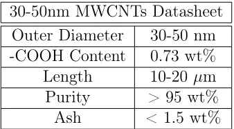
The functionalized multi-walled carbon nanotubes used in this work was supplied by Cheap Tubes, USA. The TEM micrograph and its datasheet for MWCNT is presented in figure 3.2 and table 3.1. The selection of functionalized MWCNTs is related to the mechanical properties of load transfer [140, 141] and the possibility of chemical interaction with the polymeric matrix [139].

3.3 Fabrication Technique

(51)

3.3. FABRICATION TECHNIQUE 47

Figure 3.2: TEM micrography of the supplied MWCNTs. Source: Cheap Tubes.

30-50nm MWCNTs Datasheet

Outer Diameter 30-50 nm

-COOH Content 0.73 wt%

Length 10-20 µm

Purity > 95 wt%

Ash < 1.5 wt%

Table 3.1: Manufactures datasheet for the functionalized 30-50nm MWC-NTs.

collector, applied voltage, flux rate, distance from the target, polymer concentration and solution conductivity [142, 143, 17, 18]. Recognizing this, preliminary studies were conducted to determine the optimum test parameters to achieve the project objectives. The polymer concentra-tions were defined through adaptation from previous literature publica-tions [4, 110, 2]. The solupublica-tions were tested at determined target distance and electrical field to evaluate the fiber quality of each set of parameters, while the type of collector and flux rate were fixed. The parameters used are presented in table 3.2. Hexafluoro-iso-propanol was used as solvent for the experiments, specifically due to its low boiling point (58.2 °C) and strong aﬃnity with polyamide.

(52)

in-Random PA6 Aligned PA6 Random PA6/CNT Aligned PA6/CNT

Polymer Concentration (%) 15 15 8 8

CNT Concentration (%) – – 0.2 0.2

Electrical Field (kV/cm) 0.3 - 0.8 0.3 - 0.8 0.3 - 0.8 0.3 - 0.8 Voltage (kV) 4.5 - 20 4.5 - 20 4.5 - 20 4.5 - 20 Working Distance (cm) 15 - 25 15 - 25 15 - 25 15 - 25

Flux Rate (mL/h) 0.3 0.3 0.3 0.3

Tangential Speed at the Surface (m/s)

– 5.83 – 5.83

Table 3.2: Electrospinning parameters used in the project.

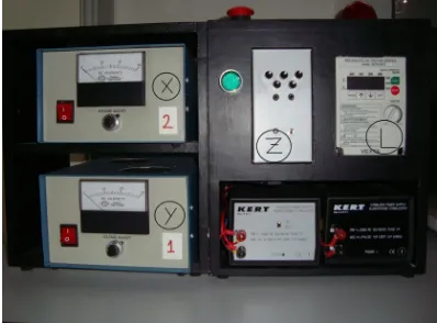
house and consists of a polymethylmetacrilate (PMMA) box that has two systems, as shown in figure 3.3, two high voltage DC generator (ES30, GAMMA High Voltage Instruments), which generates high voltage from 0 to 30 kV and two syringe pumps (MA 1 70-2208, Harvard Apparatus). The control panel is presented in figure 3.4.

(53)

3.4. CHARACTERIZATION METHODS 49

!

Figure 3.3: Electrospinning safety box, S1 shows the static system and S2 the dynamic system.

3.4 Characterization Methods

3.4.1 Carbon nanotubes analyses

3.4.1.1 Transmission electron microscopy - TEM

Transmission electron microscopy (CM12, Philips) was employed to eval-uate the quality of the supplied carbon nanotubes. MWCNTs were sus-pended in HFIP and subsequently deposited into a TEM grid.

3.4.1.2 X-Ray photoelectron spectroscopy - XPS

(54)

!

Figure 3.4: Apparatus control box.

at 0.05 eV. As the samples are conductive, they did not require charge compensation which led to an energy resolution of 0.3 eV.

3.4.2 Nanofiber morphology

3.4.2.1 Scanning electron microscopy - SEM

The fiber network morphologies were observed using SEM (Supra 40, Zeiss) in terms of fiber quality and presence of defects. The samples were gold sputtered before observation. The diameter distribution of the fibers was determined by the measurement of 30 individual nanofibers from the SEM images using image analysis software (Image J, National Institutes of Health/USA). Measurements were random performed on fibers in five diﬀerent regions of the micrograph.

3.4.2.2 Transmission electron microscopy - TEM

(55)

3.4. CHARACTERIZATION METHODS 51

observation.

3.4.2.3 Atomic force microscopy - AFM

Nanofiber topography was evaluated by AFM (NT-MDT Solver, Ze-lenograd) analysis in semi contact mode with tips of 40 nm curvature radius at 150 kHz resonant frequency. The fiber profile was extracted from the AFM images.

3.4.3 Thermal analysis

3.4.3.1 Diﬀerential scanning calorimetry - DSC

Diﬀerential Scanning Calorimetry (DSC) was employed in order to detect the influence of the filler and process on the melting and crystallization behaviour of the resulting material and to detect the presence of residual solvent. The tests were carried out on PA6 and PA6/CNT reinforced composites by using a diﬀerential scanning calorimeter (Mettler DSC30, Mettler Toledo, USA). Measurements were performed under nitrogen flow of 100 ml/min. Two consecutive heating curves were performed: first the samples were heated at a rate of 5 °C/min from 0 °C to 300 °C and then cooled till 20 °C at 5 °C/min, the second heating curve followed the same parameters as the previous. The melting enthalpy (∆Hm) was determined from the corresponding peak areas in the heating and cooling thermograms. The crystallinity content (Xc) was calculated by the application of equation 3.1.

Xc= ∆H

(∆H0)·wP (3.1)

(56)

190 J/g [144, 145], and wP is the weight fraction of polymer in the composites.

3.4.4 Mechanical analysis

The methods available to measure the mechanical properties of elec-trospun nets derive from the techniques applied for films and textile ma-terials. Nowadays, it is still not available a standard that regulates the procedures to carry out these measurements. Therefore, some caution in interpreting the data is warranted. Several parameters can influence the mechanical properties such as homogeneity and polydispersity of the fibers, type of solvent, presence of imperfections or defects [146, 3]. Thus, it is diﬃcult to compare diﬀerent studies and/or materials, and a correct experimental procedure should be described.

3.4.4.1 Tensile analysis

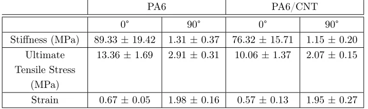
Tensile analyses were carried out for PA6 and PA6/CNT composite networks. Tests were conducted in a universal testing machine (4502, Instron) with 10 mm/min cross-head speed rate and 25 mm gauge length. The networks were cut into rectangular sheets of 5 x 35mm. The analisys of the tensile behavior was performed in two main directions according to the spinning direction, 0° and 90°. Tensile stress of each sample was calculated on the nominal cross-section area which neglects the presence of voids. Five samples of each network at both angles were submitted to the test.

3.5 Biological Evaluation

(57)

evalu-3.5. BIOLOGICAL EVALUATION 53

ation of the tested materials. Osteoblasts are responsible for bone for-mation, more specifically for the mineralization of the osteoid matrix. In essence, osteoblasts are sophisticated fibroblasts that express all genes that fibroblasts express with the addition of the genes for bone sialopro-tein and osteocalcin[147]. Fibroblasts are responsible to maintain the structural integrity of connective tissues by continuously secreting pre-cursors of the extracellular matrix. Fibroblasts secrete the prepre-cursors of all the components of the extracellular matrix, primarily the ground substance and a variety of fibres. The composition of the extracellular matrix determines the physical properties of connective tissues.

3.5.1 Protein adsorption analyses

3.5.1.1 Protein adsorption

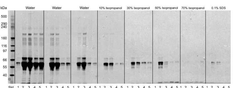
The samples were incubated for 30 min with 500µL culture medium at 37°C. The incubation period, volume, and sample dimension (10 mm of diameter) were selected to match the cell seeding conditions. The TCP well surface was used as control for all analyses. After incubation, the medium was removed and the samples were gently washed with deionized water, placed into clean TCP well and subjected to the proper protein desorption procedure. Two procedures were used to analyse the pro-tein adsorption, the qualitative total desorption and the propro-tein binding strength. For a qualitative measure of protein desorption, the samples and control were submitted to a 1 hour incubation in 0.1% of SDS at 37

(58)

to the materials for 20 min at room temperature while the SDS wash lasted for 1 hour at 37 °C under static conditions.

3.5.1.2 Electrophoresis

One-dimensional (1D) electrophoresis was performed to characterize the protein desorption from the networks and controls. The desorbed pro-teins were freeze-dried and resuspended in sample buﬀer (NuPAGET M

LDS Sample Buﬀer, Invitrogen, Italy). Six microliters of each resus-pended sample were then loaded on a sodium dodecyl sulfate polyacry-lamide electrophoresis gel (NUPageT M _{Novex 3–8% (Tris-acetate),}

In-vitrogen, Italy). The selected gel is suitable for the detection of high-molecular weight (40–500 kDa) proteins. Each gel was loaded with two molecular weight protein standards (HiMarkT M _{and SeeBlu}T M _Plus2,

In-vitrogen, Italy), fresh culture medium (1:20 in sample buﬀer) and inactive fetal bovine serum (1:40 in sample buﬀer) as control lanes. The gels were run in an XCell SureLockT M _{Midi-Cell (Invitrogen, Italy) at 150 V}

con-stant voltage. After electrophoresis, the gels were stained following the manufactures protocol using a silver-based stain (ProteoSilverT M_,

Sigma-Aldrich, Germany) or a comassie-blue based stain (ImperialT M_{, Pierce,}

USA) and further digitalized with an imaging system (GEL LOGIC 200, Kodak, USA).

3.5.2 Cell seeding and culture

(59)

3.5. BIOLOGICAL EVALUATION 55

Samples were rinsed 3 times with sterilized PBS and allowed to dry under the hood. Samples were pre incubated in 0.5 ml of medium for 30 minutes at 37°C and 5% CO2 before cell seeding to allow protein adsorption.

The MG63 and MRC5 medium were prepared from RPMI 1640 medi-um (ECB9006L, Euroclone, Italy) supplemented with 10% inactive fetal bovine serum, 1% glutamax, 1% non essential amino acids, 1% antibiotic and 1% sodium pyruvate. Phenol red free medium was used in order to avoid interference with the proliferation assay as recommended from the supplier.

Cells were seeded onto 4 identical samples for each analysis at a con-centration of 8.9 · 103_cells/cm2 _and ₃_.₂_· ₁₀4_cells/cm2 _{for MG63 and}

MRC5, respectively. The seeding concentration was defined considering the kinetics of proliferation of each cell line. Fresh culture medium was replaced every 2 days. Culture times were 3, 7 and 14 days. The morphol-ogy of the adhered cells was observed using SEM for each culture time. Cell viability was evaluated by confocal microscopy, while proliferation was assessed by alamar blue analysis.

3.5.3 Cell proliferation

(60)

was measured in two diﬀerent wavelenghs, 570 nm and 620 nm, which corresponds to the absorbance of resorufin and the background, respec-tively.

The acquired absorbance was treated to have the reduction percent-age of resazurin by the living cells. Equation 3.2 was used to calculate a correction factor in order to eliminate the eﬀect of the oxidation of alamar blue solution and the reduction percentage was calculated by the application of equation 3.3.

Ro= AO570nm

AO620nm (3.2)

AR570nm =A570nm−(A620nm·Ro)·100 (3.3)

where, Ro is the correction factor;AO570nmthe absorbance of oxidized

form at 570 nm; AO620nm the absorbance of oxidized form at 620 nm; AR570nm the percentage of reduced resazurin into resorufin; A570nm the

measured absorbance at 570 nm andA620nm the measured absorbance at

620 nm.

3.5.4 Cell viability

(61)

3.6. STATISTICAL ANALYSIS 57

3.5.5 Cell morphology

The networks for SEM observation were fixed and dehydrated after de-fined culture periods as follows: the samples were soaked in Glutaralde-hyde 25% in Cacodylic buﬀer 0.1M for 30 minutes at 4°C, then rinsed in Cacodylic buﬀer 0.1M for 3 times. Dehydration was conducted as follows: samples were soaked for 10 minutes in ethanol solutions of concentration 30%, 50%, 70%, 90% and 20 minutes in 100%, then allowed to dry under the hood. The samples were gold sputtered before observation.

3.6 Statistical Analysis

(62)

(63)

Chapter 4

RESULTS AND DISCUSSION

4.1 Carbon Nanotubes Analysis

Carboxyl functionalized MWCNT were used in this research. The mor-phology and functionalization were controlled as preliminary studies.

The morphology was accessed by TEM analysis and the result is present in figure 4.1. It was observed that there is a large diameter dispersion as well as the presence of defects on the nanotubes walls. The defects are probably the consequence of the functionalization process.

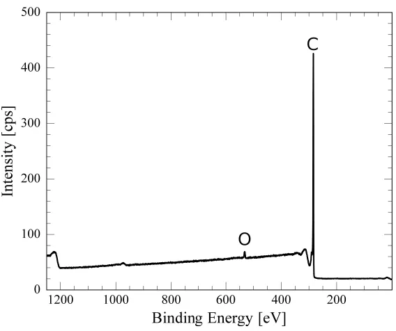
In order to evaluate the functionalization claimed from the supplier, an XPS analysis was carried out. The XPS survey spectra of the nan-otubes is presented in figure 4.2. The carbon presence is evidenced at 284 eV while the oxigen appears at 530 eV. The carbon and oxigen peak areas have been fitted in order to evaluate the presence of the specific bonds. The carbon and oxigen fitting are presented in figures 4.3 and 4.4, respectively. The quantitative analysis done by the fitting of the peaks is presented in table 4.1. The analysis has shown that the atomic abundance of oxygen is approximately 6.54%, from which 3.53% refers to hydroxyl groups, 2.19% represent the carboxyl groups and 0.81% of water.

(64)

Figure 4.1: TEM image of the supplied multi-walled carbon nanotubes.

(65)