Università degli Studi di Trento Facoltà di Scienze Matematiche Fisiche e Naturali
Tesi di Dottorato di Ricerca in Fisica
Ph.D. Thesis in Physics
Quantum Monte Carlo Methods applied
to strongly correlated and highly
inhomogeneous many–Fermion systems
Candidate:
Supervisor:
Lucia Dandrea
Dr. Francesco Pederiva
Contents
1 Introduction 1
1.1 Laterally confined 2D Electron Gas . . . 2
1.2 Fermionic Shadow Wave Function . . . 6
2 Quantum Monte Carlo Methods 9 2.1 Variational Monte Carlo . . . 9
2.1.1 The Metropolis algorithm . . . 10
2.2 Diffusion Monte Carlo . . . 10
2.2.1 Description of DMC method . . . 11
2.2.2 Importance sampling . . . 12
2.2.3 Fixed–node approximation . . . 13
2.2.4 Technical details . . . 14
2.2.5 Forward-walking algorithm . . . 15
3 Method details for the confined two dimensional electron gas 17 3.1 Hamiltonian . . . 17
3.2 Trial wavefunction . . . 18
3.2.1 Optimization trial wavefunction . . . 19
3.3 Ewald Summation . . . 21
3.3.1 The procedure . . . 22
3.3.2 Solution of Poisson equation for ρ2 . . . 24
3.3.3 Solution of Poisson equation for ρ1 . . . 25
3.3.4 Average potential in the cell equal to zero . . . 25
3.3.5 Computation ofξ . . . 26
3.3.6 Implementation of Ewald Summation . . . 26
3.4 CHAMP . . . 27
3.4.1 Particularly noteworthy features of CHAMP . . . 27
4 Ground state properties of the laterally confined 2D electron gas 29 4.0.2 Results at~ω0 = 4meV . . . 30
CONTENTS
4.1 Overview . . . 42
5 Fermionic Shadow Wave Function 45 5.1 Shadow Wave Function . . . 45
5.2 Antisymmetric Shadow Wave Function . . . 47
5.3 Fermionic Shadow Wave Function . . . 48
5.3.1 FSWF problems . . . 49
5.3.2 Proposed solution to FSWF sign problem . . . 50
5.4 Ground state properties of 3He vacancies . . . . 51
5.4.1 Technical details . . . 51
5.4.2 Results . . . 53
6 Conclusions and perspectives 59
Acknowledgements 63
List of Figures 65
List of Tables 69
Chapter 1
Introduction
The theoretical understanding ofmany-body systems is one of main challenges in
quantum Physics. It is already impossible to solve a system with more than four particles using analytic methods. Theoretical physics has made many efforts in order to develop tools to study many-body systems. To overcome the limit of applicability of exact analytical solution it is necessary to use some approxi-mations. An outstanding examples is given by Mean-field theory (MFT). The main idea of MFT is to replace all interactions to any one body with an average or effective interaction. This reduces any multi-body problem into an effective one-body problem. However one MFT limitation is that it is not possible to study systems with local dis-homogeneities, like solids.
Methods trying to compute on exact solution of Schroedinger equation for a given Hamiltonian Hˆ are much more demanding. For a limited number of
particles (N <10), it is possible to compute eingenvalues and eigenstates of Hˆ by computing its matrix elements on a given basis, and then diagonalizing the matrix. For larger system the direct knowledge of the wavefunction is not pos-sible, and stochastic techniques, known under the names of (Quantum) Monte Carlo methods must be used.
There are many variants of QMC methods with different possible applica-tions. In this work we focus on two types: Variational (VMC) and Diffusion (DMC) Monte Carlo methods. VMC and DMC are very used and tested meth-ods. The scientific community knows very well their limits and capacities. These two methods are particularly indicated in order to study the ground state prop-erties of a quantum system at temperature of 0K. However they can not give
information on time evolution of the system.
In this work we studied two different kinds of systems. The first is a two– dimensional electron gas laterally confined by a harmonic potential in the ef-fective mass–dielectric constant approximation. The second is a solid 3He in
presence of defects.
1.1. LATERALLY CONFINED 2D ELECTRON GAS
computational challenge they pose.
First of all studying Fermion system by QMC methods means to face the notorious sign problem. In the first system, there is the classical sign problem
of the DMC method, which can be milded in our case by a well known approxi-mation, thefixed–node approximation. The second system requires a variational
treatment in which we have a integral sign problem. Computing the mean value of the energy, using Fermionic Shadow Wave Functions (FSWF), positive and negative terms in the integral appear. Summing these terms, the positive con-tributions tends to cancel the negative ones. However the noise is too large to obtain a useful signal.
Furthermore the electrons system is confined, strongly correlated and we do not know the equilibrium phase a priori. All these aspects make difficult the computation. We also studied the equation state of 3He solid with a vacancy,
meaning that the system is highly dis-homogeneous making it necessary to find a wavefunction which can describe a dis-homogeneous phase.
The effort of this work is to find a solution to some technical problem that you have when you want to study a strongly correlated and highly inhomogeneous many–Fermion systems with the Quantum Monte Carlo Methods. In this way we want to try to say more about these systems.
1.1
Laterally confined 2D Electron Gas
The two dimensional (2D) electron gas laterally confined by some potential is a fundamental model in many-body physics since the progress in nanostructure technology has allowed the fabrication of 2D quantum stripes.
There are many different kinds of objects that go under the name of quantum wires. Our interest is focused on semiconductor quantum wires.
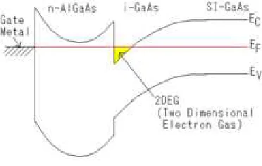
It is possible to create a two-dimensional electron gas (2DEG) at junction in-terface of two semiconductor (see fig. 1.1). In particular, a kind of quantum wires
CHAPTER 1. INTRODUCTION
Figure 1.2: A one dimensional quantum wire realized at the edge of a two di-mensional electron gas [1]
is obtained by etching a semiconductor quantum well, obtained at the junction between differently doped semiconductors (e.g. GaAs/AlGaAs) (see figure 1.2). Split-gates technique is a method for creating a smooth one-dimensional con-striction in a 2DEG. When a negative voltage Vg is applied to a lithographically defined pair of Schottky split-gates above a GaAs/AlxGa1−xAs heterostructure,
shown in Fig. 1.3, the 2DEG is depleted from beneath the gates and a 1D channel is left defined between them. If the elastic mean free path le is much greater than the width W and length L of the channel, transport through the 1D constriction is ballistic and the differential conductance, G(Vg)=N(2e2/h),
is quantized, where N is the number of transmitted 1D subbands.
Experiments in these nanostructures have pointed out the quantization of the conductanceGin units of2e2/h, which reflects the number of active channels
in the transport measurements[4, 5, 6]. A conductance structure close to G = 0.7(2e2/h) has been observed in many cases[7, 8, 2, 3, 9, 10] (see figure 1.4).
These experiments are made on quantum point contacts (which are quantum wires of length l = 0) or on quantum wires with length of few µm, formed
in GaAs/AlxGa1−xAs heterostructures, generally in the absence of a magnetic
field. The intensity of this structure changes from0.5(2e2/h)to0.7(2e2/h), that
1.1. LATERALLY CONFINED 2D ELECTRON GAS
Figure 1.3: (left) Schematic of a split-gate device, where S and D represent the source and drain contacts [2]. (Right) Gate configuration used to define the wire. The top gate and side gates are separately adjusted to control the electron density and the wire confinement potential [3].
18, 19], or of Wigner crystallization of the confined electron gas at low density[20] or of a Tomonaga-Luttinger liquid behavior[21, 22, 23, 24, 25, 26, 27, 28, 29, 30]. All these results are based on specific models or approximations like, for exam-ple, the local spin density functional theory.
In this thesis we present a fixed node diffusion Monte Carlo calculation of the ground state of a 2D quantum stripe of infinite length and finite width described by the 2D Hamiltonian of N interacting electrons laterally confined by a parabolic potential. The extension of the stripe in the third dimension is neglected, as in most theoretical descriptions. This approximation is jus-tified by the fact that the confinement of the electron in the quantum well is extremely strong, and at all relevant densities only one subband is occu-pied. We calculate the ground state energy for the unpolarized and fully spin-polarized liquid phases and solid phase. Previous Monte Carlo calculations of quasi-unidimensional systems have been performed by Casula, Sorella, and Sen-atore [31]. The authors in that case considered a one dimensional system with an interaction that effectively includes the width of the wire. However, be-ing the Hamiltonian one-dimensional, no phase transitions can occur in the system, according to the Lieb–Mattis theorem[32]. Our calculation being fully two–dimensional, makes it possible to discuss relative stability of phases with different symmetry.
We met many technical problems to implement this model.
CHAPTER 1. INTRODUCTION
Figure 1.4: Experimental result[7]. Conductance of a l = 0.5µm quantum wire
as a function of side gate voltage forVT =560 mV-1500 mV (right to left). Inset:
Conductance as a function of side gate voltage for VT=1.5 V
convergence. Then many tests were necessary to optimize the Ewald break up.
We made many checks on wavefunction and also we verified the ergodicity of the system was guaranteed.
We did not have a direct comparison with another computational model that could verify the correctness of our work. We made all the possible tests to assert our work could explain this confined two-dimensional electron system.
The system was studied as a function of rs (0.5≤rs ≤7) and~ω0 (~ω0 =2, 4, 6 meV).ω0 is the confining parameter andrs is the one–dimensional
Wigner-Seitz parameter rs = 1/2ρ1D. The values of rs correspond at values of ρ
1D in the range 104 −106cm−1. The combination of ω
0 with ρ1D reproduces the two–dimensional density of the experiments [7, 2, 3].
The results show us how the system tends to become more localized increas-ing the confinincreas-ing parameter ω0. In this range of ω0 for rs > 3 we found the
1.2. FERMIONIC SHADOW WAVE FUNCTION
1.2
Fermionic Shadow Wave Function
The Fermionic Shadow Wave Function is an extension, for Fermion system, of Shadow Wave Functions (SWF)[33]. SWF is a particular class of many– body wave functions employed to study bosonic systems. Its main property is that it describes a disordered phase and/or a crystalline phase of a quantum system within the same functional form, which is manifestly translationally invariant. In this way, it is possible to study non–homogeneous systems and phase transitions. Using SWF, it is possible for example to study the equilibrium point between two different phases of the system, which naturally emerges from the wavefunction.
SWF were largely used to study properties of liquid–solid 4He [34] and 3He
[35], system with phase coexistence [36] or presence of defects or impurities [37] and superfluid liquids with vortex excitations [38].
As it will be explained in the following chapters, the use of SWF for Fermions presents severe technical difficulties in some cases. In the thesis the first applica-tion of a FSWF antisymmetrized on the auxiliary degree of freedom is presented, in wich some relevant physical properties has been computed successfully.
The general form of FSWF would be useful to describe many–body systems with the coexistence of different phases as well in the presence of defects or im-purities, but it requires overcoming a significant sign problem. As an application, we studied the energy to activate vacancies in solid 3He.
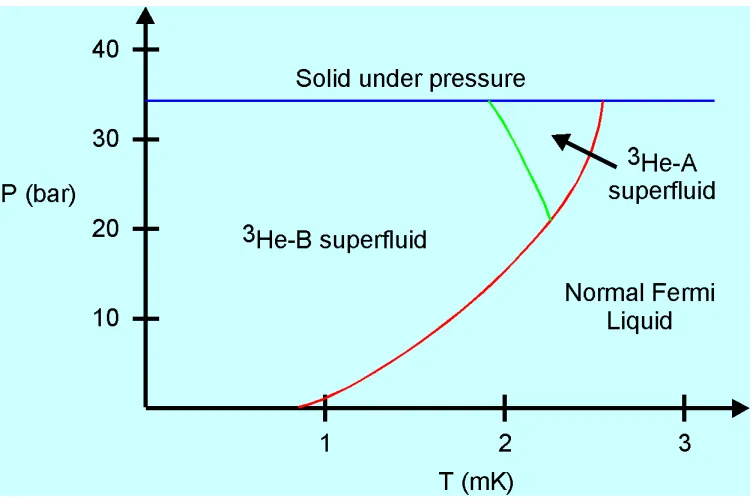
3He is a very strongly interacting quantum system. In figure 1.5 the 3He
phase diagram is represented. Experimentally one finds that for temperatures in the mK region, two superfluid phases appear in the liquid, and a quasi-antiferromagnetic ordered bcc phase shows up in the solid, which changes into a normal antiferromagnetic when the magnetic field is increased.
We focus our attention on the solid phase. In VMC or DMC the solid phase is generally described by product of Gaussian orbitals. For a Fermion system it is necessary, in principle, to use a determinant of Gaussians in order to consider the antisymmetry of the system. In a regime of strong localization the determinant of Gaussians is essentially equivalent to a product of localized orbitals because of the rare occurrence of exchange among particles on different lattice sites. For this reason, the simulation of a homogeneous quantum crystal, even in presence of the Pauli principle, does not represent a significant challenge.
When the lattice symmetry is locally broken by the presence of the vacancy, exchange among the atoms in the crystal becomes much more effective. The phenomenon can also be viewed as a “motion” of the vacancy through the crystal itself. The effect due to the Fermion nature of 3He become then evident at the
CHAPTER 1. INTRODUCTION
Figure 1.5: Phase diagram of 3He below 3 mK. The solid phase appears only
above the pressure of 34 bar. At high temperatures the liquid is in the normal Fermi state. There are two superfluid phases, A and B.
energy. FSWF is the only wavefunction that can account for all these characters of the system.
Our goal was find a way to make the calculations feasible. For solid 3He
Chapter 2
Quantum Monte Carlo Methods
TheMonte Carlo methods[39] are a set of algorithms, which use the random (or
pseudo–random) numbers in order to solve mathematical problems. The Monte Carlo methods are mainly used to compute integrals. The main difficulty in solving an integral with the standard methods is the computation effort in-creases exponentially with dimensionality of the integration domain. MC avoids this problem. In fact the evaluation of a multidimensional integral is made by sampling the integrand and averaging the sampled values. The statistical error in the value of integral decreases as the square root of the number of sampling points used, regardless of dimensionality. This is a consequence of the central limit theorem.
In particular we are interested to introduce the Quantum Monte Carlo Method (QMC) for study quantistic system. We start introducing the Varia-tional Monte Carlo (VMC) and the Diffusion Monte Carlo (DMC) method. In
chapter 5 we talk about theFermionic Shadow wave function FSWF, which are
a special way to do VMC.
2.1
Variational Monte Carlo
The Variational Monte Carlo (VMC) method is based on variational principle. The expectation value of Hˆ evaluated with a trial wavefunction ψT provides a
rigorous upper bound on the exact ground-state energy E0:
EV =
R
ψ∗
T(R) ˆHψT(R)dR
R
ψ∗
T(R)ψT(R)dR
≥E0 (2.1)
where R = (~r1, ~r2, ..., ~rN) is the 3N-dimensional vector and ~ri is the position
2.2. DIFFUSION MONTE CARLO
Metropolis algorithm [40] and the integral 2.1 is rewritten in this way:
EV =
R
|ψT(R)|2hψT(R)−1HψTˆ (R)idR
R
|ψT(R)|2dR (2.2)
where |ψT(R)|2 becomes the probability density and ψT(R)−1HψTˆ (R) is the
quantity to accumulate. In VMC the configurations R are sampled following a distribution probability.
VMC is often used to optimize trial wavefunction.
2.1.1
The Metropolis algorithm
The Metropolis algorithm (M(RT)2) has the great advantage of allowing an
arbitrarily complex distribution to be sampled in a straightforward way, without knowledge of its normalization.
Suppose we define a 3N− dimensional vector R, a particular value of R is called awalker orconfiguration. The probability density of finding the system in
the configurationRwill be denoted byP(R)(whereP(R)≥0andR
P(R)dR= 1). The M(RT)2 generated the sequence of sampling points Rm by moving the
single walker according the following rules [41]: 1) Start the walker at a random position R.
2) Make a trial move to a new position R′ chosen from some probability
density function T(R′ ←R).
3) Accept the trial move with probability
A(R′ ←R) =Min
1,T(R←R
′)P(R′)
T(R′ ←R)P(R)
If the trial move is accepted, the pointR′ becomes the next point on the
walk, otherwise the next point remains R.
4) Return to step 2 and repeat.
2.2
Diffusion Monte Carlo
A practical method of studying the properties of a many body quantum system is the Diffusion Monte Carlo (DMC) algorithm. DMC is a stochastic algorithm based on transforming the analytic continuation of the Schrödinger equation in imaginary time into a diffusion equation.
CHAPTER 2. QUANTUM MONTE CARLO METHODS
2.2.1
Description of DMC method
The Schrödinger equation in imaginary time τ =it is given by
−∂τ∂ ψ(R, τ) =Hψ(R, τ) (2.3)
A formal solution written in integral form is
ψ(R, τ) =
Z
G(R, R′, τ)ψ(R′,0)dR′ (2.4) where the kernelG(R, R′, τ)is the Green’s function of the operatorH+ ∂
∂τ, and it can be expressed as the matrix element
G(R, R′, τ) =hR|e−(H−E0)τ|R′i=Xe−(En−EO)τφ∗
n(R)φn(R′) (2.5) where φn is a complete set of eigenvectors of H.
One starts choosing a trial wavefunction ψT, which is not orthogonal to the ground state of the system. It is possible to write ψT as a linear combination of φn:
ψT(R) =cnφn(R) (2.6)
The evolution in imaginary time of ψT is:
ψT(R, τ) =e−(H−E0)τψ(R,0) =e−(H−E0)τcnφn(R) (2.7)
Considering the limit for τ → ∞ you obtain the ground state.
The non-interacting Hamiltonian
Let us consider the non interacting Hamiltonian of N particles with mass m
H0 =−
X
i ~2
2m∇
2
i (2.8)
the corresponding kernel G0 is a Gaussian with variance proportional to √τ:
G0(R, R′, τ) =
m
2π~2τ
32N
e−m(R−R ′)2
2~2τ (2.9)
this equation describes the Brownian diffusion of N particles.
It possible to implement this equation writing the wavefunction as a set of discrete sampling points, the walkers:
|ψ(R)i=X
k
2.2. DIFFUSION MONTE CARLO
where |xki=δ(R−Rk)is eingenfunction of position.
The evolution in imaginary time step ∆τ is: ψ(R, τ + ∆τ) =X
k
G(R, Rk, τ + ∆τ) (2.11)
This set of Gaussian functions represents a distributions ofwalkers. In the limit
of τ → ∞these points represent the ground state of H0.
The interacting Hamiltonian
In order to solve the equation 2.3 with the Hamiltonian:
H =−X
i ~2
2m∇
2
i +V(R) (2.12)
it is necessary to use the Trotter formula in this way:
G(R, R′,∆τ)≈e−
“V(R)+V(R′)
2 −ET
”
∆τ
G0(R, R′,∆τ) (2.13)
that introduces an error in ∆τ (O(∆τ3)).
Now the kinetic term is separated from the potential term and the wavefunction can be rewritten
ψ(R, τ + ∆τ) = m 2π~2τ
32NZ
e−m(R−R ′)2
2~2τ e−
“V(R)+V(R′)
2 −ET
”
∆τ
ψ(R′, τ)dR′ (2.14) The kinetic part gives a diffusion term, the potential part gives a branching
term:
w=e−
“V(R)+V(R′)
2 −ET
”
∆τ
(2.15) w represents a weight of the Green’s function.
The integral 2.14 is solved with Monte Carlo method by propagating the parti-cles according the diffusion term. Instead the branching term gives the proba-bility of multiply a configuration at the next step.
2.2.2
Importance sampling
Solving equation 2.3 by a purely diffusive random-walk process with branching is rather inefficient, because the weight term 2.15 could have large fluctuations. For example, ifV(R)is the electron-electron and electron-ion Coulomb potential
the branching term can diverge ±∞. This leads to a large fluctuations in the number of walkers and to a slow convergence when calculating averages [42].
CHAPTER 2. QUANTUM MONTE CARLO METHODS
Storer,1971; Ceperley and Kalos, 1979; Reynolds et al., 1982). The idea is to
multiply the both member of eq. 2.3 for a known ψT(R)and rewrite it in terms
of a new probability distribution f(R, τ) = ψT(R)ψ(R, τ). After rearranging
terms we obtain
−∂f(R, τ)
∂τ =−D∇
2f(R, τ) + (EL(R)
−ET)f(R, τ) +D∇ ·(f(R, τ)FQ(R))
(2.16) where D=~2/2m. Here the “quantum force” FQ(R) is defined as:
FQ(R) = ∇ln|ψT(R)|2 = 2∇ψT(R)
ψT(R)
and in the coefficient of the branching termEL is thelocal energy defined as:
EL = HψTˆ (R)
ψT(R)
Under the assumption that ψT is not orthogonal to the ground state φ0, in the
limit of τ → ∞ the distribution f(R, τ) becomes proportional to ψT(R)ψ0(R).
The three terms on the left-hand side of equation 2.16 represent a diffusion, drift and branching process respectively. An approximate Green’s function for small time-step ∆τ of such equation is given by the product of the individual diffusion, drift and branching Green’s function[42]:
˜
G(R′, R,∆τ) = m 4Dπ∆τ
32N Z
dR”e »
−(R4′−DR∆”)2τ
–
(2.17)
× δ(R”−R−DFQ(R)∆τ)
× exp
−∆τ
1
2[EL(R) +EL(R
′)] −ET
2.2.3
Fixed–node approximation
In the DMC algorithm the wavefunction ψ(R) is represented by a population
density, therefore the algorithm is well defined only if ψ(R)is defined positive.
ψ(R)may also be everywhere negative, since the overall phase of the
wavefunc-tion is arbitrary. This implies that a wavefuncwavefunc-tion has to be without nodes. This is a problem if we are interested in Fermionic system. The Fixed-node
ap-proximation [42, 41] is a method for dealing with the fermion antisymmetry. Although not exact, it gives ground-state energies that can be proved to be an upper bound of the true ground state, which is always lower than the variational upper bound given by the wavefunction used to impose the nodal surface.
2.2. DIFFUSION MONTE CARLO
wavefunction has a nodal structure that divides the space in many positive and negative pockets. The Fixed-node approximation consists in keeping the walkers in the pockets with the same sign. One scatters DMC walkers throughout the configuration space and moves them in the usually way. After every DMC move the sign of the trial wavefunction is checked. If the walker has crossed the trial nodal surface it is deleted or the move is rejected if an acceptance-rejection scheme is used.
If the nodes of the trial wavefunction are exact the result is the exact ground-state energy, otherwise an upper bound of the ground state energy of the Fermions is obtained. The challenge of a Fixed-node DMC calculation is find a trial wavefunction which has a nodal structure as close as possible to the real nodal structure. Finding a good nodal structure is necessary in order to minimize the nodal-error.
2.2.4
Technical details
In DMC calculation many technical details have to be considered.
Time step error
Developing DMC method is necessary to separate in the propagator the kinetic terms from potential term using Trotter formula (see Eq. 2.13). This step intro-duce a time step error. In order to evaluate this error it is necessary repeat the
same calculation with different value of∆τ. The best value is the extrapolation at∆τ = 0.
Population bias
In DMC the population is a set of walkers. The number of walkers change during the computation due to the branching. In order to avoid wide fluctuations of population the weight may be corrected in this way:
w= N0
N exp(−∆τ(EL−E0)) (2.18)
where N is the number of walker and N0 is the prefixed number of walker.
This correction allows to controll the population, but that modifies the sam-pling so it introduces a population error. Therefore it is necessary extrapolate the energy value in function of 1/N for high value of N.
Mixed estimator
In order to evaluate a generic operatorsO(R), which do not commute with the
CHAPTER 2. QUANTUM MONTE CARLO METHODS
result. The mixed estimator consists in taking twice DMC result minus VMC result, in this way you obtain the mean value of O(R)on the ground state:
hOi= 2hφ0|O|ψTi − hψT|O|ψTi+ϑ(α2) (2.19)
The bias affecting such estimate is of the second order in α, where α is defined by φ0 =ψT +αψα.
2.2.5
Forward-walking algorithm
An other method to evaluate operators, which do not commute with the Hamil-tonian, is the Forward-walking [43, 44] algorithm.
The pure estimator of an operator O(R)may be written as:
hO(R)i=
D
φ0
O(R)
φ0
ψT
ψT
E
D
φ0
φ0
ψT
ψT
E (2.20)
φ0(R)/ψT(R) can be obtained from the asymptotic offspring of the R walker.
The idea is to assign to each walker Ri a weight W(Ri) proportional to its number of descendants, W(Ri) =n(R, τ → ∞). Eq. 2.20 becomes:
hO(R)i=
P
iO(R)W(Ri)
P
iW(Ri)
(2.21)
Chapter 3
Method details for the confined
two dimensional electron gas
3.1
Hamiltonian
In order to determine the Hamiltonian of the system we start from a two di-mensional electron gas of density ρ2D = 1/πa2 in the effective mass-dielectric
constant approximations. In this thesis we will consider effective units, assum-ing ǫ = 1 and m∗ = 1. The density of the gas is parametrized by the
effec-tive Wigner-Seitz radius in effeceffec-tive atomic units r2D
s = a/a∗0. For reasons of
convenience, in the simulations we prefer to rescale all lengths in terms of a one-dimensional Wigner-Seitz parameter rs =L/2N whereN is the number of electrons, andLis the length of the wire, which by this scaling depends only on the number of electrons, and not on the density. The one– and two–dimensional densities are related to each other as ρ1D = ρ2Dw(ρ1D), where w is an esti-mate of the width of the wire. A possible definition of w(rs) is given by twice
the distance from the center of the wire at which the transverse density decays to one half of the value at the center. Similarly we can relate r2D
s and rs as r2D
s ∼
p
2rsw(rs)/π. With this choice of the length units, energies are given
in effective Rydbergs. The Hamiltonian of theN electrons in the stripe is then defined as follows:
H=−1
r2
s N
X
i=1 ∇2i +
N
X
i=1
ˆ
ω02yi2+ 2
rs N
X
i,j=1
VCoul(ri,rj). (3.1)
The harmonic confinement parameter ωˆ0 =ω0rs is scaled consistently with the
coordinates. Note that for independent electrons this choice of the confinement would give a width of the wire w(rs)∝ 1/rs, therefore corresponding to
summa-3.2. TRIAL WAVEFUNCTION
tion (see section 3.3). The assumption is that the diverging Coulomb repulsion is compensated by the interaction with a jellium of positive charge. We then consider a 2D array of such stripes in the limit of infinite separation.
3.2
Trial wavefunction
An important step in order to make a good DMC computation is find the a good trial wavefunction. A good choice ofψT leads to smaller statistical error for the same amount of sampling. For a Fixed-node DMC computation the choice of ψT becomes important in order to minimize the node-error.
In this work we used a trial wavefunction of the following form:
ψT(r1. . .rN) =
N
Y
i=1
u(yi)
N
Y
i<j
J(rij)Det↑φα(rβ)Det↓φα(rβ) (3.2) The Jastrow factor (JF) J(rij)is a simplified version of the form used in ref.
[45]. The JF reduces the statistical error in both VMC and DMC for a given number of Monte Carlo steps. Otherwise the JF leaves the fixed-node DMC energy unchanged because the node of the trial wavefunction is not altered. In the original form the JF contains three terms: electron-electron Jee, electron-nuclei Jen and electron-electron-nuclei Jeen. We only use the term Jee:
J(rij) =exp(fee) =exp b1R(rij)
1 +b2R(rij)
+
Nord
X
p=2
bp+1Rp(rij)
!
(3.3)
The scaling function R(r) is given by r/(1 +κr). Nord, the order of the
poly-nomials, is taken to be 5. The number of parameters to be optimazed is re-duced by the imposition of the electron-electron cusp condition: b1 must be 1
for antiparallel-spin electrons and1/3 for parallel spin electrons.
The one body factor u(y) = exp(−c1y2) is a Gaussian which is used to
fine-tune an overall correction to the lateral width of the wavefunction.
The single particle functions are solutions of the non–interacting Hamilto-nian:
φα(r) = ψhol (y)φ(x) (3.4)
where ψl
ho(y) are eigenstates of the harmonic oscillator of frequency ωˆ0′. The
single particle functions φ(x) can be chosen to enforce the symmetry of the
state considered. For simulating the liquid phase we useφ(x) = exp(−ikx). The
momentumkis consistent with the periodicity of the system:k =±n2π/L, with
CHAPTER 3. METHOD DETAILS FOR THE CONFINED TWO DIMENSIONAL ELECTRON GAS
density of the system, and must be determined from the Fermi energy of the N particles. In the simulations we assumed that the filling of the bands is the same for the interacting and non-interacting electrons. We checked this assumption by computing the DMC energy for different fillings of the bands, always obtaining the lowest energy for the filling predicted for independent electrons.
In order to study the occurrence of a localized phase we implemented another set of single particle orbitals φ(x, xj) = exp[−c(x − xj)2], where xj are the
localization centers located at y = 0 and distanced by L/N. Because we are considering an antisymmetrized product of such orbitals, this choice does not automatically correspond to constraining an electron around a given lattice site. If the orbitals are overlapping with each other an exchange of electrons is always possible.
In this thesis we used four wavefunctions (a), (b), (c) and (d). The differences among wavefunctions are summarized in table 3.1. The polarized wavefunction is defined as the product of two determinants, Det↑φα(rβ)Det↓φα(rβ), one con-taining the coordinates of N/2particles with spin up and the other containing
the coordinates of N/2 particles with spin down. The polarized wavefunction
includes a single determinant, in which there are the coordinates of all particles (with the same spin).
(a): φα(rβ) =ψl
ho(yβ) exp(−ikαxβ), unpolarized liquid (b): φα(rβ) = exp[−c(xβ −xα)2] exp[−c2(yβ)2], unpolarized solid
(c): φα(rβ) =ψhol (yβ) exp(−ikαxβ), polarized liquid
(d): φα(rβ) = exp[−c(xβ −xα)2] exp[−c2(yβ)2], polarized solid
Table 3.1: Differences among wavefunctions (a), (b), (c), (d).c2 = ˆω′+c.
3.2.1
Optimization trial wavefunction
In this work we optimize the parametersc,c1 andωˆ′0, appearing in the
wavefunc-tion , by directly computing the energy for different values. Instead the Jastrow parameters are optimized using the Newton and Linear methods [46, 47]
intro-duced by C. J. Umrigar and C. Filippi.
3.2. TRIAL WAVEFUNCTION
Newton optimization method
The energy E(p) is expanded to second order in the parameter p and p0, E[2](p) = E0 +
Nopt
X
i=1
gi∆pi+1 2 Nopt X i=1 Nopt X j=1
hij∆pi∆pj (3.5)
where the sums are over all the parameters to be optimized, ∆pi =pi−p0i are the components of the vector of parameter variations∆p,gi are the components of the energy gradient vector g and hij are the elements of the energy Hessian matrix h:
gi =
∂E(p)
∂pi
hij =
∂2E(p)
∂pi∂pj
(3.6)
Imposition of the stationary condition on expanded energy expression, ∂2E(p)
∂pi∂pj =
0, gives the following standard solution for the parameters variations:
∆p=−h−1·g (3.7)
where h−1 is the inverse of the Hessian matrix. In practice, eq. 3.7 gives the parameter variations ∆p that are used to update the current wavefunction,
|ψ0 >→ |ψ(p0+ ∆p)>. This procedure has to be interacted until convergence
is reached.
The Newton method is stabilized adding a positive constant adiag to the diagonal of the Hessian matrix h
hij →hij +adiagδij
As adiag is increased the parameter variation ∆p becomes smaller and rotates from the Newtonian direction to the steepest descent direction.
In eq. 3.7 we used as gi the components of the energy gradient vector and hij the elements of the energy Hessian matrix. It is possible resolve the eq. 3.7 using gradient and Hessian of energy variance.
Linear optimization method
The idea is to expand a normalized wavefunction |ψ(p)i to first order in the
parameters p around the current parameterp0:
|ψlin(p)i=|ψ0i+
Nopt
X
i=1
∆pi|ψii (3.8)
where the wavefunction at p = p0 is simply |ψ(p0)i = |ψ0i = |ψ0i (chosen to
CHAPTER 3. METHOD DETAILS FOR THE CONFINED TWO DIMENSIONAL ELECTRON GAS
orthogonal to |ψ0i.
|ψii=
∂|ψ(p)i
∂pi
p=p0
=|ψii −S0i|ψ0i (3.9) where S0i = hψ0|ψii. The minimization of the energy calculated with this
lin-ear wavefunction leads to the stationary condition of the associated Lagrange function:
∇p[hψlin(p)|Hˆ|ψlin(p)i −Elinhψlin(p)|ψlin(p)i] = 0 (3.10) The Lagrange function is quadratic inpand equation 3.10 leads to the following generalized eigenvalue equation:
H·∆p=ElinS·∆p (3.11)
His th matrix of the HamiltonianHˆ in the(Nopt+1)-dimensional basis consist-ing of the current normalized wavefunction and its derivatives, S is the overlap matrix of this(Nopt+ 1)-dimensional basis and∆pis the(Nopt+ 1)-dimensional vector of parameter variation with∆p0 = 1. The linear method consists of
solv-ing equation 3.11 for the lowest eigenvalue and associated eigenvector ∆p.
The simple procedure of incrementing the set of parameters p by ∆p is p0 = p0 + ∆p. It works for the linear parameters but it is not guaranteed
to work for nonlinear parameters if the linear approximation of eq. 3.8 is not good. The Jastrow factor has nonlinear parameters. In this case is necessary to modify the standard procedure. A right choice of normalization of wavefunction can avoid the problem.
As the Newton optimization method it is possible to stabilize the minimiza-tion by adding a positive constant adiag to the diagonal ofHexcept for the first element.
3.3
Ewald Summation
3.3. EWALD SUMMATION
in one dimension. In this work we build a theoretical solution to the quasi-one dimensional case of the Ewald summation. Our task is to solve the problem for a 2D system of electrons with finite extent in one dimension and periodic in the other.
3.3.1
The procedure
Consider a 2D system periodic in one dimension and of finite extent in the other dimension, made of N electron and a uniform canceling background charge. The charge distribution, if there were one electron at rn in the unit periodic cell is:
ρ(r−rn) =X
R
δ(r−rn−R)−ρbackground
where R = nL is the lattice translation vector with n = 0,±1,±2..., L is the
periodicity of the system and ρbackground is the background distribution charge (which makes each and every cell neutral).
What we want is to write the potential generated from this charge distribu-tion in a useful way, due to the problems mendistribu-tioned in the introducdistribu-tion. The Ewald Method consists in adding and subtracting to the charge distribution of
the electron an array of Gaussian function, centered in rn+R. This is just
adding something which is zero. So we have:
ρewald(r,rn) =ρ(r,rn) = ρ1(r,rn) +ρ2(r,rn)
ρ1(r,rn) =
1
µ√π
3
X
R
e−(
r−rn−R)2
µ2 −ρbackground
ρ2(r,rn) = X
R
δ(r−rn−R)−
1
µ√π
3
e−(r−rnµ2−R)2
!
where µ is an arbitrary parameter that determines the width of the Gaussian distribution.
As it is possible to see in ρ2(r,rn), the extra distribution acts like a
screen-ing positive charge. In this way, if µ is big enough, the interaction between neighboring electrons becomes a short range interaction due to the screening.
The potential due to ρ1(r,rn) is calculated in reciprocal space and the one
due to ρ2 in the real space, both with the Poisson equation:
∇2Φewald(r,rn) =−4πρewald(r,rn)
Solution of Poisson equation for ρ2(r,rn) in real space gives:
Φ2(r,rn) = X
R
1−erf|r−rn−R| µ
CHAPTER 3. METHOD DETAILS FOR THE CONFINED TWO DIMENSIONAL ELECTRON GAS
Steps of the solution are shown in Section 3.3.2. Solution of Poisson equation for ρ1(r,rn) in reciprocal space k= (kx, ky)(where kx = 2Lπn, n=±1,±2, ... is
discrete due to the periodicity along x direction) gives:
Φ1(r,rn) =
4
L
X
kx>0
cos(kx(x−xn))
Z +∞
0
dky 1
|k|erf c
µ|k|
2
cos(ky(y−yn))
Steps of the solution are shown in Section 3.3.3
Now we can write the Ewald potential in this way:Φewald(r,rn) = Φ1(r,rn)+
Φ2(r,rn) +A(rn) where the last term is added because the average potential
in the cell must be zero, due to the neutrality of charge in the cell (see Section 3.3.4). Considering N electrons in the cell, the potential Φ(r) generated in r
by the N charges is found by superposing all the potentials for each charge component:
Φ(r) =
N
X
n=1
Φewald(r,rn)
The potential acting on the chargerj is:
Φ(rj) =
N
X
n=1
Φewald(rj,rn)− lim r→rj
1
|r−rj|
where the second term is the divergent part of the self interaction of the electron inrj with its own potential. It is possible to rewrite it in the following way:
Φ(rj) =
N
X
n6=j
Φewald(rj,rn) +ξ(rj)
where ξ(rj)is the potential acting on the electron at rj due to its own periodic
images and canceling background (see Section 3.3.5).
ξ(rj) = lim
r→rj
Φewald(r,rj)−
1
|r−rj|
(3.12)
So the full Ewald potential energy appearing in Hamiltonians is the sum of the potential acting on all the N electron
Uewald(r1, ...,rN) = e 2
2
N
X
j=1
Φ(rj) = e 2 2 N X j=1 N X
n6=j
Φewald(rj,rn) +ξ(rj) !
3.3. EWALD SUMMATION
3.3.2
Solution of Poisson equation for
ρ
2The equation to be solved is:
∇2Φ2(r,rn) =−4π X
R
δ(r−rn−R)−
1
µ√π
3
e−
(r−rn−R)2
µ2
!
with the condition that Φ2 goes to zero at infinity.
The equation splits into two equations. The first is the part with theδ function. The solutionΦ2delta is:
Φ2delta(r,rn) = X
R
1
|r−rn−R|
The second part is with the Gaussian function with solution Φ2Gaus . Due to symmetry reason, the solution Φ2Gauss does not depend on the angles, so the Laplacian is:
∇2 = 1
r2
d dr
r2 d dr
If we look for a solution of the form:
Φ2Gauss(r) = χ(r)
r
the equation becomes:
d2
dr2χ(r) =
4
µ3√πr
X
R
e−(
r−rn−R)2
µ2
A solution of this equation with the correct boundary condition is:
χ2Gauss(r) =−
X
R
erf
|r−rn−R|
µ
erf(x) = √2
π
Z x
0
dte−t2 therefore the solution for ρ2 is:
Φ2(r,rn) = X
R
1−erf|r−rn−R| µ
CHAPTER 3. METHOD DETAILS FOR THE CONFINED TWO DIMENSIONAL ELECTRON GAS
3.3.3
Solution of Poisson equation for
ρ
1It is possible to calculate this solution starting from the 2D result:
2π A
X
k
1
|k|erf c
µ|k|
2
e−ik·(r−rn)
where A is the area of the 2D plane.
We proceed therefore by considering a set of parallel quasi one-dimensional wires, distributed over the 2D layer. The distance between the wires is c. In order to obtain the result of quasi one-dimensional case it needs to consider a unit cell of areacL in which there is a single wire. Then you evaluate the limit c→ ∞of the previous equation:
Φ1(r,rn) = lim
c→∞ 2π cL X kx 1
|k|erf c
µ|k|
2
e−ik·(r−rn)=
= 1 L X kx Z +∞ −∞ dky 1
|k|erf c
µ|k|
2
e−ik·(r−rn) =
= 4
L
X
kx>0
cos(kx(x−xn))
Z +∞
0
dky 1
|k|erf c
µ|k|
2
cos(ky(y−yn))
3.3.4
Average potential in the cell equal to zero
We have to calculate the average potential in the cell and add a function A to make it zero:
hΦewald(x, y) +Aiϕ(x,y) = 0
whereϕ(x, y)is the wavefunction of the positive background in the cell, i.e. the
ground state of an harmonic oscillator along y direction (since the binding on the y direction is considered harmonic) times a plane wave along x direction (since along x direction the system is homogeneous):
ϕ(x, y) = √1
L
α
π
14
e−α2y2eikxx α= mω
~
So you obtain the follow expression for A:
A=A(rn) =−1
L
α
π
12 Z +
L
2
−L2
dx
Z +∞
−∞
dyX
R
1−erf|r−rn−R| µ
|r−rn−R| e −αy2
3.3. EWALD SUMMATION
3.3.5
Computation of
ξ
ξ(rj)is the potential acting on the electron atrj due to its own periodic images
and canceling background:
ξ(rj) = lim
r→rj
Φewald(r,rj)−
1
|r−rj|
= = X
R6=0
1−erf|Rµ|
|R| −limt→0
erft µ
t +A(rj) +
+4
L
X
kx>0
Z +∞
0
dky 1
|k|erf c
µ|k|
2
= = X
R6=0
1−erf|Rµ|
|R| −
2
µ√π +A(rj) +
4
L
X
kx>0
Z +∞
0
dky 1
|k|erf c
µ|k|
2
3.3.6
Implementation of Ewald Summation
The implementation of Ewald Summation was very difficult. First of all it is necessary to tabulate all the contributions in order to minimize the computing time machine, in particular the integral terms.
The calculation of A(rn) is very heavy, because wide oscillation in the
inte-grand make difficult to reach a convergence. After many attempts the problem was resolved using the Gauss-Laguerre Quadrature method. The idea of Gaus-sian Quadratures [52] is rewrite the a defined integral in the following way:
Z b
a
W(x)f(x)dx≈ N−1
X
j=0
wjf(xj) (3.13)
We can arrange the choice of weights wj and abscissas xj to make the integral exact for a class of integrands. In numerical analysis Gauss-Laguerre quadrature is an extension of Gaussian quadrature method for approximating the value of integrals of the following kind:
Z ∞
0
e−xf(x)dx (3.14)
In this case
Z ∞
0
e−xf(x)dx≈ n
X
i1
wif(xi) (3.15)
CHAPTER 3. METHOD DETAILS FOR THE CONFINED TWO DIMENSIONAL ELECTRON GAS
The second important step is to choose the optimal value for µ. That is a parameter modulating the screening effect of Gaussians. We chose the value of µthat minimizes the dependence of energy on the number of electron N.
We found that a good value ofµisL/5, whereLis the side of the simulation cell. This value does not differ from the heuristically determined value that is commonly presented for 2D and 3D simulations.
We chose to perform the simulations using different numbers of electrons in order to have a direct controll on how much the potential contribution depend onN. In the table 4.1 there is the value of energy atrs=5 for different numbers of electron,N=50, 75, 98. This example shows the energy depends on N and it involves a change in energy of order10−4. The important aspect is the difference
in energy if you make a computation with N =73 or 75 is smaller then error.
3.4
CHAMP
The program used to study the ground-state properties of the two-dimensional electron gas laterally confined was based on CHAMP1. CHAMP is a Quantum
Monte Carlo suite of programs for electronic structure calculations on a variety of systems (atoms, molecules, clusters, solids and nanostructures) written by Cyrus Umrigar, Claudia Filippi and, with smaller contributions, by a few others. CHAMP is presently a suite of 11 programs that have the following 3 basic capabilities:
1. Optimization of many-body wave functions by variance minimization (FIT)
2. Metropolis or Variational Monte Carlo (VMC)
3. Diffusion Monte Carlo (DMC).
In order to use Champ for compute the laterally confined 2D electron gas it was necessary to make substantial changes in the code. The bigger change was the introduction of Ewald summation (see section 3.3) for the potential computation. Then we fixed the periodicity only in one dimension using the
periodic boundary condition. We wrote the wavefunction (see section 3.2), except
the Jastrow factor.
3.4.1
Particularly noteworthy features of CHAMP
Efficient wavefunction optimization by the variance-minimization method. For finite systems the capability exists to optimize not only the Jastrow part of the
3.4. CHAMP
wavefunction but the determinantal part (CI coefficients, orbital coefficients and orbital exponents) as well.
a) Optimized Trial Wave Functions for QMC calculation [53].
b) A Method for Determining Many-Body Wavefunctions[54],
A variety of forms of the Jastrow factor that introduce e-n, e-e and e-e-n correlations (e=electron, n=nucleus), including forms that are systematically improvable (within the constraint due to using no more than e-e-n correlations) and that obey all three types of cusp conditions exactly. For large systems the option exists to use Jastrow functions that go exactly to a constant beyond some distance, thereby improving the scaling of the computer time with system size[53, 54, 55]
An accelerated Metropolis method that allows one to make very large moves and still have a high acceptance, resulting in very short autocorrelation times. The gain, compared to other Metropolis methods is particularly large when pseudo potentials are not used[56, 57].
Chapter 4
Ground state properties of the
laterally confined 2D electron gas
Simulations have been performed using different numbers of electrons, at dif-ferent values of the density, parametrized by the Wigner-Seitz radius rs, and at different value of confinement parameter ω0. The confinement parameter has
been chosen to be ~ω0 = 2,4,6meV (= 0.338,0.674,1Ry∗).
As previously exposed in the chapter 3, in a QMC simulation it is neces-sary to choose a good trial wavefunction, to be used as importance function and starting point for the projection. For the confined 2D electron gas, we use the combination of plane wave, Gaussian orbitals and Jastrow correlations de-scribed in chapter 3. The structure of the wavefunction is the same both for the antiferromagnetic and for ferromagnetic state considered. For the case in which electrons are localized (Wigner crystal states) the plane waves are replaced by Gaussians in the longitudinal direction.
When the lateral confinement is strong it is possible to identify a single relevant parameter determining the properties of the wire, i.e. is the ratio between the gap in the single particle levels in the harmonic confining po-tential, and the Fermi energy of the electrons in the longitudinal direction CF = 2m~ω0/~2k2
F[59], which in effective atomic units reduces to 32r2sω0/π2.
Therefore, at least in the strongly one-dimensional regimeCF >>1, the results
should approximately be independent of the specific value of ω0 and scale as a
function ofCF. However, this is not true at high densities, where more than one harmonic oscillator band is occupied.
We thoroughly studied the dependence of the results of the finite size, that might come from the use of Ewald sums for the potential energy. At the end of this analysis we concluded that forN ≥74such effects are already well reduced.
4.0.2
Results at
~
ω
0= 4
meV
In Tab. 4.1 we report the energy per electron computed with N = 74 and 98
electrons at different values of rs.
For the unpolarized liquid phase the number of harmonic oscillator bands used in the wavefunctions is 3 for rs = 0.5, and 1 for rs > 1, while for the
polarized liquid phase we fill 5 bands for rs = 0.5, 2 for rs = 1, and one for
rs>1. In the localized phase we consider localized orbitals, and we assume that the correct density is reached by varying the parameters of the Gaussians.
As it can be seen, at high densities (rs <3) the ground state is an unpolarized
liquid. In particular forrs≤1theCF parameter is rather small, and the system has a two–dimensional character.
For rs ≥ 5 the ground state is found to be the spin–polarized, with an
energy gap of the order 1mRy∗. However, for a given polarization, the liquid
and crystal phases have extremely close energies. This very small difference (<0.1mRy∗) might be taken as a conservative estimate of the fixed node error,
suggesting that the energy gap between the polarized and unpolarized phases is robust. However, it is not possible within our current numerical accuracy to draw a definite conclusion about the occurrence of Wigner crystallization.
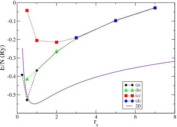
In Fig. 4.1 we report the computed energies, together with the fit of the total energy according to the Tanatar-Ceperley[60] functional in the range of 2D densities corresponding to an estimate of the electron density of the wire. As it can be seen, at low values of rs, the energy of the electrons in the wire becomes closer and closer to that of the equivalent homogeneous 2D system. The discrepancies are due to the approximate way in which the width of the wire is determined. On the other hand, the figure clearly displays that in the highrs regime the energies of the four phases considered strongly deviates from the 2D value, and tend to collapse on a single value, consistently with the fact that we are approaching an effective 1D regime (CF → ∞).
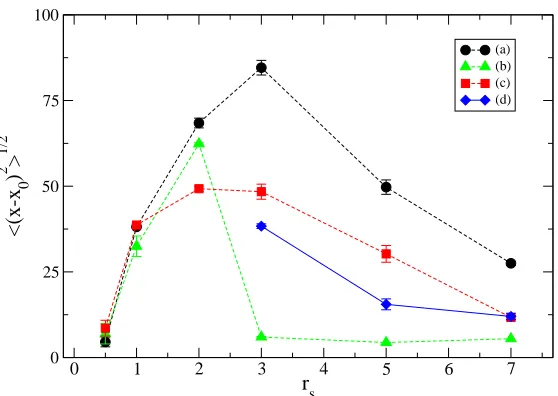
A problem occurring in QMC simulations of quasi 1D systems is the lack of ergodicity due to the extremely low exchange rate between electrons[31]. We tried to assess the existence of this drawback in our 2D simulations. This was achieved both by direct inspection, i.e. by checking the diffusion of close pairs of electrons, and looking at the Monte Carlo mean square diffusion of the electrons along the wire, estimated by:
h(x−x0)2i= 1
NM M
X
j=1
N
X
i=1
[xj,i(τ)−x0,i]2 (4.1)
where x0,i and xj,i(τ) (with τ = M∆τ, ∆τ is the time step used in the DMC
CHAPTER 4. GROUND STATE PROPERTIES OF THE LATERALLY CONFINED 2D ELECTRON GAS
N,rs 0.5 1 2 3 5 7
50 (a) -0.095596(6)
74 (a) -0.5288(4) -0.36810(5) -0.26760(3) -0.19458(3) -0.09549(1) -0.026681(7)
98 (a) -0.5513(4) -0.36800(8) -0.26750(3) -0.19453(2) -0.09544(1) -0.026791(7)
50 (b) -0.09647(1)
74 (b) -0.4163(6) -0.26527(3) -0.19465(1) -0.096476(8) -0.027629(5)
98 (b) -0.3979(8) -0.26518(3) -0.19460(1) -0.096491(7) -0.027634(5)
49 (c) -0.09787(1)
73 (c) -0.0424(4) -0.20522(5)∗ -0.21482(1) -0.19067(1) -0.097797(6) -0.028524(4)
97 (c) -0.0443(4) -0.20697(8) -0.21524(1) -0.19077(1) -0.097695(6) -0.028500(4)
49 (d) -0.09772(1)
73 (d) -0.18999(1) -0.097671(6) -0.028423(6)
97 (d) -0.19000(1) -0.097673(5) -0.028405(4)
Table 4.1: Total energy per electron (in effective Rydberg) for a laterally confined two dimensional electron gas with~ω0=4meV. (a): unpolarized liquid wavefunc-tion. (b): localized wavefuncwavefunc-tion. (c): polarized liquid wavefuncwavefunc-tion. (d): polar-ized solid wavefunction. (∗): N=74.
0 2 4 6 8
rs -0.5
-0.4 -0.3 -0.2 -0.1 0
E/N (Ry)
(a) (b) (c) (d) 2D
Figure 4.1: Total energy per electron (in effective Rydberg) for a laterally con-fined two dimensional electron gas. Dots: unpolarized fluid; triangles: unpolar-ized crystal; squares: polarunpolar-ized fluid; diamonds: polarunpolar-ized crystal. The full line is the energy of the 2D system at a value ofr2D
0 1 2 3 4 5 6 7 rs
0 25 50 75 100
<(x-x
0
)
2 >
1/2
(a) (b) (c) (d)
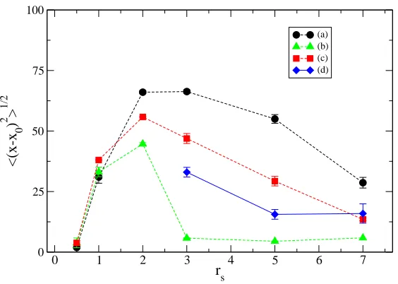
Figure 4.2: QMC diffusion of the electrons in the wire (in units of a∗ 0) as a
function of rs at ~ω0 = 4meV. The points display the computed diffusion for the unpolarized liquid (dots), polarized liquid (squares), localized (triangles) and polarized solid (diamonds) phases.
In Fig. 4.2 we report the evaluation of this quantity as a function of rs for the four phases considered. In this picture thexcoordinates are in units of a∗
0 in
order to avoid the rescaling effect of box size. Forrs≤2the diffusion of electrons
is very active. The dependence on rs (almost linear for the unpolarized liquid phase) is given by the increased size of the wire in the longitudinal direction. This is a clear sign of the fact that electrons are allowed to almost freely diffuse for the whole length of the wire. Forrs≥ 3the diffusion ceases to increase. When
using localized orbitals, it is clear how the diffusion converges to a constant value much lower than the values seen in the liquid phase, indicating that electrons remain strongly localized around lattice sites.
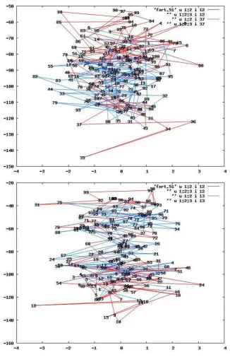
In figure 4.3 there are two examples of the random walks described by two neighboring electrons during the simulation. Both figures represent the liquid phase at low density (rs = 5) for pairs of electrons with opposite spin (fig. 4.3,
CHAPTER 4. GROUND STATE PROPERTIES OF THE LATERALLY CONFINED 2D ELECTRON GAS
Figure 4.3: Electron displacements in liquid phase at low density (rs = 5) for
In Fig. 4.4 we report the transverse electron density for two different values of rsand the transverse jellium density. The picture shows how the system becomes effectively narrower with increasing rs. For rs = 0.5 the system is almost two
dimensional, in agreement with the fact that the energy of the confined system approaches the energy of the 2D system. For lower densities, the effect of the confinement on the energy becomes stronger and stronger.
-4 -2 0 2 4
y
0 0.1 0.2 0.3 0.4
transverse density
rs=1
rs=5
jellium
Figure 4.4: Transverse density in the confined 2D electrons gas. The density computed by DMC is compared with the "jellium" density, i.e. from the density given by the ground state solution of the confining harmonic potential. Curves are given forrs = 1(dotted and dashed-dotted line), andrs= 5(full and dashed
lines). y is given in units of a∗ 0
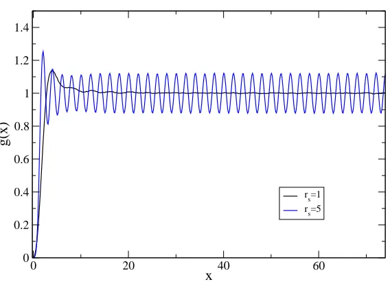
In figure 4.5 the pair correlation function, g(x), for rs= 1 andrs = 5is
dis-played. g(x)is computed along the longitudinal coordinate x and integrated in the transverse coordinatey. Decreasing the density,g(x)shows wide oscillations.
In figure 4.6 we show the electron spin density r(x), computed in the
longi-tudinal direction, for two different densities (rs= 1and rs = 5), and computed
using localized wavefunction. r(x) is the probability that an electron with a
fixed spin is at position x. We find that by increasing the electron density, the number of exchanges increases. At high density (rs = 1) the electron density displays a modulation, but electrons are spread all over the wire. At low density (rs= 5) electrons are clearly localized around lattice sites.
CHAPTER 4. GROUND STATE PROPERTIES OF THE LATERALLY CONFINED 2D ELECTRON GAS
0 20 40 60
x 0
0.2 0.4 0.6 0.8 1 1.2 1.4
g(x)
rs=1 rs=5
Figure 4.5: Pair correlation function for rs= 1 and rs= 5.
-2 -1.5 -1 -0.5 0 0.5 1 1.5 2 x
0 0.005 0.01 0.015 0.02 0.025 0.03
spin density
rs=1, spin down rs=1, spin up rs=5, spin down rs=5, spin up rs=5 polarized solid
4.0.3
Results at
~
ω
0= 2
meV and
~
ω
0= 6
meV
We studied the equation of state for two other values of confining parameterω0.
In order to understand how our model behaves changing the lateral confinement. We proceeded to study the system for ~ω0 = 2,6 meV in the same way we did for ~ω0 = 4 meV.
The same algorithm to fill up the orbitals of wavefunction was employed. At ~ω0 = 2meV for the unpolarized liquid phase the number of harmonic oscillator bands used in the wavefunctions is 4 for rs = 0.5, 2 for rs = 1, and one for
rs ≥ 2, while for the polarized liquid phase we fill 7 bands for rs = 0.5, 3 for
rs= 1, and one forrs>1. At~ω0 = 6meV, for the unpolarized liquid phase the number of harmonic oscillator bands used in the wavefunctions is 3 forrs = 0.5,
and one for rs ≥ 1, while for the polarized liquid phase we fill 5 bands for
rs= 0.5, 2 for rs= 1, and one forrs >1.
We report in table 4.2 the equation of state for ~ω0=2meV and in table 4.3 the equation of state for~ω0=6meV. Comparing tables 4.2, 4.1 ,4.3 it is possible to observe that increasing ω0 the density at which the liquid phase ceases to
exist shifts to higher density and at rs ≥3the system is always polarized.
A deeper analysis shows that at ~ω0 = 6meV for rs < 3 the system is still liquid. It is possible to understand this observation by looking at the figures 4.7, 4.8 and 4.9.
Fig. 4.7 shows the QMC diffusion of the electrons in the wire as a function of rs at ~ω0 = 6meV. The black dots and the green triangles are very close for rs <3, meaning that the system behaves in a similar way either using the
unpolarized liquid wavefunction or solid wavefunction. The wavefunction for a solid is built starting from orbitals localized on given lattice sites. However, the Pauli principle (implemented in the construction of a Slater determinant) yields the electron exchange, that is frequent at high densities.
N,rs 0.5 1 2 3 5 7
72 (a) -0.7687(4) -0.4636(1)
73 (a) -0.33693(2) -0.27728(1) -0.20086(1) -0.148749(6)
96 (a) -0.7449(4) -0.4605(3)
98 (a) -0.33705(2) -0.27726(2) -0.20080(1) -0.14871(1)
74 (b) -0.4679(7)* -0.33125(2) -0.27458(1) -0.203092(7) -0.149657(4)
98 (b) -0.33136(2) -0.27460(2) -0.203087(7) -0.149658(5)
73 (c) -0.4181(4) -0.3737(2) -0.25989(1) -0.26576(1) -0.203839(7) -0.150329(4)
97 (c) -0.3720(3) -0.25876(1) -0.26574(1) -0.203812(7) -0.150316(4)
73 (d) -0.26494(1) -0.202332(7) -0.147502(7)
97 (d) -0.26496(1) -0.202330(7) -0.147564(7)
CHAPTER 4. GROUND STATE PROPERTIES OF THE LATERALLY CONFINED 2D ELECTRON GAS
N,rs 0.5 1 2 3 5 7
74 (a) -0.3040(4) -0.28103(5) -0.16975(4) -0.08584(3) 0.03041(1) 0.108615(6)
98 (a) -0.3042(4) -0.28217(5) -0.16974(4) -0.08564(3) 0.03052(1) 0.108659(6)
74 (b) -0.3951(6) -0.2960(3) -0.16970(4) -0.08619(2) 0.029973(8) 0.108301(5)
98 (b) -0.3816(6) -0.2922(2) -0.08627(2) 0.029964(9) 0.108300(4)
73 (c) 0.3158(4) -0.12901(2) -0.08457(1) 0.028429(7) 0.107428(5)
74 (c) -0.02518(5)
97 (c) 0.3346(5) -0.12951(2) -0.08452(1) 0.028459(7) 0.107441(4)
98 (c) -0.02575(6)
73 (d) -0.08385(1) 0.028588(4) 0.107971(4)
97 (d) -0.08382(1) 0.028608(7) 0.107958(4)
Table 4.3: Total energy per electron (in effective Rydberg) for a laterally confined two dimensional electron gas with~ω0=6meV. (a): unpolarized liquid wavefunc-tion. (b): localized wavefuncwavefunc-tion. (c): polarized liquid wavefuncwavefunc-tion. (d): polar-ized solid wavefunction.
0 1 2 3 4 5 6 7
rs 0
25 50 75 100
<(x-x
0
)
2 >
1/2
(a) (b) (c) (d)
Figure 4.7: QMC diffusion of the electrons in the wire (in units of a∗ 0) as a
0 20 40 60
x
0 0.5 1 1.5
g(x)
(a) (b)
h - ω
0=6 meV, rs=1
Figure 4.8: Pair correlation function for rs = 1 at ~ω0 = 6meV. The points display the g(x) computed with the unpolarized liquid (a) and solid (b)
wave-function.
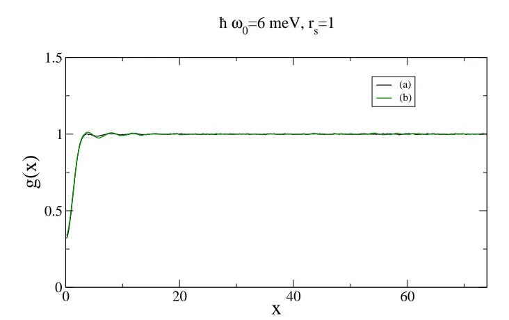
In Fig. 4.8 and 4.9 the pair correlation function g(x) for rs = 1 and rs = 3
at ~ω0 = 6meV are shown. In both figures there are the g(x) computed using unpolarized liquid and localized wavefunction. At rs = 1 a different choice of wavefunction along x (plane wave or Gaussians) leads to a pair distribution function g(x) that it always displays the typical features of a liquid. For rs= 3
(Fig. 4.9) the difference between the pair functions computed starting from different wavefunctions is evident and then the solid structure ofg(x)computed
with unpolarized solid wavefunction becomes clear.
In figure 4.10 we also report the QMC diffusion of the electrons at ~ω0 =
2meV. This picture confirms the liquid–like behavior of the system for rs ≤ 3.
For the unpolarized liquid phase the diffusion linearly increases with rs indi-cating that on average the exchange of electrons is very active. For rs >3 the
diffusion ceases to increase. In the solid phase it is clear how for rs > 2 the
diffusion ceases to increase and converges to constant values much lower (about one order of magnitude) than the values seen in the liquid phase, indicating that electrons are strongly localized around lattice sites. The polarized liquid phase shows a strange behavior as a function ofrs. There is a strong connection between the wavefunction parameters and the QMC diffusion. For example the low value of QMC diffusion at rs = 2 for polarized liquid phase is due to the
choice of parameter c1 (u(y) = exp(−c1y2), see Eq. 3.2). The parameter c1 can
CHAPTER 4. GROUND STATE PROPERTIES OF THE LATERALLY CONFINED 2D ELECTRON GAS
0 20 40 60
x
0 0.5 1 1.5
g(x)
(a) (b)
h - ω
0=6meV, rs=3
Figure 4.9: Pair correlation function for rs = 3 at ~ω0 = 6meV. The points display the g(x) computed with the unpolarized liquid (a) and solid (b)
wave-function.
0 1 2 3 4 5 6 7
r
s
0 25 50 75 100
<(x-x
0
)
2 >
1/2
(a) (b) (c) (d)
Figure 4.10: QMC diffusion of the electrons in the wire (in units of a∗ 0) as a
low value of c1. However, a small variation in c1 implies an high variation in
the walker’s capacity to diffuse. So this parameter is useful, but very difficult to use.
At ~ω0 = 2 meV, as at ~ω0 = 4 meV, we do not report the unpolarized solid value at rs = 1, due to unresolved computational difficulties. At rs = 1
the system is a unpolarized liquid. Using a solid wavefunction we are not able to obtain a stable value for the energy.
Another previous feature is the energy value at ~ω0 = 2 meV and rs = 0.5, E/N = −0.7687(4) Ry∗. This value looks unexpected because it is lowest of
![Figure 1.2: A one dimensional quantum wire realized at the edge of a two di-mensional electron gas [1]](https://thumb-us.123doks.com/thumbv2/123dok_us/857591.2080024/9.595.223.415.118.340/figure-dimensional-quantum-wire-realized-edge-mensional-electron.webp)
![Figure 1.4: Experimental result[7]. Conductance of a l = 0.5µm quantum wireas a function of side gate voltage for VT =560 mV-1500 mV (right to left)](https://thumb-us.123doks.com/thumbv2/123dok_us/857591.2080024/11.595.184.459.127.329/figure-experimental-result-conductance-quantum-wireas-function-voltage.webp)