METHODOLOGY
Development of the Australian Cancer Atlas:
spatial modelling, visualisation, and reporting
of estimates
Earl W. Duncan
1,2, Susanna M. Cramb
1,3, Joanne F. Aitken
3,4,5,6,7, Kerrie L. Mengersen
1,2and Peter D. Baade
3,4*Abstract
Background: It is well known that the burden caused by cancer can vary geographically, which may relate to dif-ferences in health, economics or lifestyle. However, to date, there was no comprehensive picture of how the cancer burden, measured by cancer incidence and survival, varied by small geographical area across Australia.
Methods: The Atlas consists of 2148 Statistical Areas level 2 across Australia defined by the Australian Statistical Geography Standard which provide the best compromise between small population and small area. Cancer burden was estimated for males, females, and persons separately, with 50 unique sex-specific (males, females, all persons) cancer types analysed. Incidence and relative survival were modelled with Bayesian spatial models using the Leroux prior which was carefully selected to provide adequate spatial smoothing while reflecting genuine geographic varia-tion. Markov Chain Monte Carlo estimation was used because it facilitates quantifying the uncertainty of the posterior estimates numerically and visually.
Results: The results of the statistical model and visualisation development were published through the release of the Australian Cancer Atlas (https ://atlas .cance r.org.au) in September, 2018. The Australian Cancer Atlas provides the first freely available, digital, interactive picture of cancer incidence and survival at the small geographical level across Australia with a focus on incorporating uncertainty, while also providing the tools necessary for accurate estimation and appropriate interpretation and decision making.
Conclusions: The success of the Atlas will be measured by how widely it is used by key stakeholders to guide research and inform decision making. It is hoped that the Atlas and the methodology behind it motivates new research opportunities that lead to improvements in our understanding of the geographical patterns of cancer burden, possible causes or risk factors, and the reasons for differences in variation between cancer types, both within Australia and globally. Future versions of the Atlas are planned to include new data sources to include indicators such as cancer screening and treatment, and extensions to the statistical methods to incorporate changes in geographical patterns over time.
Keywords: Australian Cancer Atlas, Cancer incidence, Relative survival, Spatial smoothing
© The Author(s) 2019. This article is distributed under the terms of the Creative Commons Attribution 4.0 International License (http://creat iveco mmons .org/licen ses/by/4.0/), which permits unrestricted use, distribution, and reproduction in any medium, provided you give appropriate credit to the original author(s) and the source, provide a link to the Creative Commons license, and indicate if changes were made. The Creative Commons Public Domain Dedication waiver (http://creativecommons.org/ publicdomain/zero/1.0/) applies to the data made available in this article, unless otherwise stated.
Open Access
*Correspondence: [email protected]
3 Cancer Council Queensland, PO Box 201, Spring Hill, Brisbane, QLD 4004, Australia
Background
There is a long history of studies showing that where you live matters [1–5]. This can relate to health, economics or lifestyle. It is no different with cancer. The existence of significant geographic variation in cancer incidence and mortality is well known [6, 7], however, most anal-yses until now have been based on relatively broad or socioeconomically heterogenous geographic areas, pre-cluding detailed area-based comparisons. A number of health-related and cancer-specific interactive, online atlases have been previously released in other countries, including, for example, the Environmental Health Atlas (UK), the National Cancer Institute Cancer Atlas (USA), The Centre for Disease Control Interactive Cancer Atlas (USA), and cancer mortality maps in Spain by province and municipal level [8–11]. However to date, there has been no comprehensive atlas of cancer in Australia.
The Australian Cancer Atlas [12], launched in Septem-ber 2018, provides the first digital, interactive picture of cancer burden at the small geographical level across Australia, including modelled estimates of both cancer incidence and survival, and incorporating the statistical methodology and visualisation methods that are required for accurate estimation, interpretation and decision making.
Given the increasing number of cancer atlases avail-able internationally, the variety of statistical methods and visualisation techniques utilised, and the inferences that may be drawn from the atlas estimates by researchers, managers, and policy makers, it is our aim here to outline the rationale and development of the statistical models used for the Australian Cancer Atlas, and the method of visualising the estimates from those models. In doing so, it is hoped that these statistical and visualisation methods may be used more widely, thus creating opportunities for more direct comparisons between the geographical pat-terns of cancer burden and possible causes or risk fac-tors, both within Australia and across other countries.
Methods
Geographical areas
The geographical areas that compose the Atlas are Sta-tistical Areas level 2 (SA2s), defined by the Australian Statistical Geography Standard (ASGS) July 2011 edi-tion [13]. SA2s broadly represent communities that interact together socially and economically, and cover Australia without gaps or overlap [14]. Australian SA2s range in size from < 1 to 520,000 km2, and in 2014 had a
median population of 8991 (range 0 to 54,773). There are two main reasons for using SA2s: they provide the best compromise between small population and small area to enable modelling at a “small area” scale; and they are
the smallest geographical areas to which cancer registries routinely assign patient residence at diagnosis.
Of the 2214 SA2s covering Australia, those with no res-idential population (n = 28), no physical location (com-prising ‘Migratory–Offshore–Shipping’ and ‘No usual address’ codes for each State and Territory) (n = 18), fewer than five residents on average per year dur-ing 2010–2014 (n = 17), and those very remote islands > 500 km from the Australian mainland [Christmas Island, Cocos Island and Lord Howe Island (n = 3)] were excluded. This left 2148 SA2s for which modelled esti-mates are provided in the Atlas.
Cancer types and outcome measures
The cancer types, classified using the 2016 version of the International Classification of Diseases (ICD-10) dis-ease code (Table 1), [15] were selected based predomi-nately on those with higher numbers of diagnoses. Due to discrepancies between how the state and territory cancer registries assigned invasive status during the time period of interest (2005–2014), bladder cancer (ICD-10 C67) was excluded from the analysis. Breast cancer was restricted to females only, due to an insufficient number of breast cancers diagnosed among males for analysis. Due to reporting estimates by males, females and all per-sons separately, 50 unique sex-specific (males, females, all persons) cancer types were included in the analysis.
Incidence
Cancer incidence refers to the number of new cancer cases diagnosed within a given time period. In order to make comparisons of cancer incidence between small areas with differing population size and age structure, incidence rates were compared rather than the number of cancers diagnosed. Indirect standardisation through the standardised incidence ratio (SIR) [16] is the pre-ferred method of standardisation when there are very small numbers in some age groups, because it removes the substantial sampling variation that would be present in this situation with direct standardisation [17]. The SIR reflects the area-specific incidence rate relative to the Australian average. It is the ratio of the observed cancer cases to the expected number of cases, the latter adjust-ing for differences in population between SA2s and dif-ferences in age structure of the population within an SA2.
Survival
Atlas, relative survival estimates up to 5 years after diag-nosis were generated using the period method [19]. The relative survival models estimate the excess hazard ratio (EHR), which, for a given geographical area, is inter-preted as the risk of dying from a given cancer within 5 years after diagnosis relative to the Australian average risk [18].
Time period
To maximise the robustness of the spatial estimates due to the sparse data (Table 1), the cancer cases were aggre-gated over multiple years. For cancer incidence, the five most commonly diagnosed cancers and the category “all cancers” used data aggregated over the latest 5-year period (2010–2014), while all other cancer types com-bined cases over the latest 10-year period (2005–2014). For the cancer survival estimates, data were aggregated across the entire ‘at-risk’ time period for which popula-tion mortality data were available, namely 2006–2014. Given that the period method was being used to calculate
relative survival, cases included in the survival analyses could have been diagnosed from 2001 onwards.
Data sources
De-identified individual level data for each case of can-cer diagnosed in Australian residents during the speci-fied period were obtained from the Australian Cancer Database (ACD), which is maintained by the Austral-ian Institute of Health and Welfare (AIHW) [20]. The ACD contains records on all primary invasive cancer cases (excluding basal and squamous cell carcinoma of the skin) diagnosed in Australian residents and notified to one of Australia’s eight state and territory population cancer registries. Australia has mandatory cancer notifi-cation, ensuring virtually complete population incidence data. At the time of analysis, the ACD contained records of cases diagnosed from 1982 to 2014 (1982–2013 in New South Wales), although geographical information for cancer cases at the SA2 level was only available from 1996 onward. Cases with missing SA2 details (0.8% of all cancers) were excluded from the analyses.
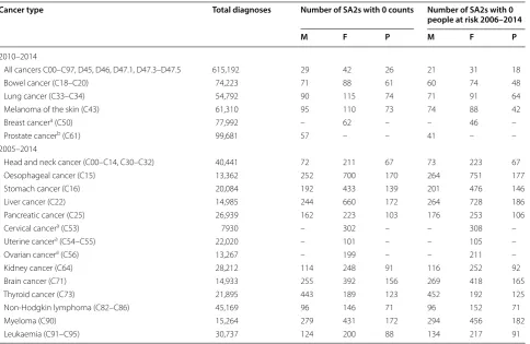
Table 1 Time period and data sparsity by type of cancer
M males, F females, P persons
a Females only
b Males only note that only the 2148 SA2s considered to have a residential population are included
Cancer type Total diagnoses Number of SA2s with 0 counts Number of SA2s with 0 people at risk 2006–2014
M F P M F P
2010–2014
All cancers C00–C97, D45, D46, D47.1, D47.3–D47.5 615,192 29 42 26 21 31 18
Bowel cancer (C18–C20) 74,223 71 88 61 60 74 48
Lung cancer (C33–C34) 54,792 90 115 74 71 91 64
Melanoma of the skin (C43) 61,310 95 110 73 74 88 42
Breast cancera (C50) 77,992 – 62 – – 46 –
Prostate cancerb (C61) 99,681 57 – – 41 – –
2005–2014
Head and neck cancer (C00–C14, C30–C32) 40,441 72 211 67 73 223 67
Oesophageal cancer (C15) 13,362 252 700 170 264 751 177
Stomach cancer (C16) 20,084 192 433 139 201 476 146
Liver cancer (C22) 14,985 244 660 172 264 728 186
Pancreatic cancer (C25) 26,939 162 223 103 176 253 106
Cervical cancera (C53) 7930 – 302 – – 308 –
Uterine cancera (C54–C55) 22,020 – 101 – – 105 –
Ovarian cancera (C56) 13,267 – 199 – – 211 –
Kidney cancer (C64) 28,212 114 248 91 116 252 92
Brain cancer (C71) 14,933 255 392 156 269 418 165
Thyroid cancer (C73) 21,895 443 189 123 452 192 125
Non-Hodgkin lymphoma (C82–C86) 45,169 96 146 71 96 152 71
Myeloma (C90) 15,264 279 431 172 294 456 182
Estimated residential population data grouped for Aus-tralia by SA2, year, sex, and 5-year age group (to 85+
years) were obtained from the Australian Bureau of Sta-tistics (ABS) [21]. These population data were only avail-able from 2001 onward.
Unit record population mortality data for all causes of death combined were only available from the Registry of Births, Deaths and Marriages [22] for the period during 2006 to 2014. The unit record data included details about sex, year of death, age, and SA2 at death.
Statistical models
Spatial smoothing
Due to the inherent variation that is associated with low numbers in small geographical areas, spatial smooth-ing was used to increase the stability of the result-ing estimates and protect confidentiality. In effect, spatial smoothing borrows information from neighbour-ing areas, seekneighbour-ing to estimate the underlyneighbour-ing rate, rather than simply reporting the more pronounced random var-iation arising from very low numbers of observed cases when there are few residents. Spatial smoothing also alleviates the effect of the somewhat arbitrary nature of boundaries defining the geographical areas.
There are several ways to carry out statistical smooth-ing. For the Atlas we used Bayesian spatial models, in particular, conditional autoregressive models. Two main advantages of this approach were that Bayesian models readily incorporate the spatial correlation between areas in a natural manner as part of the prior information, rec-ognising that adjoining geographical areas are likely to have some similar characteristics, and also that the prob-abilistic description of each of the unknown quantities provides a unique capacity to better quantify the extent of uncertainty around the spatial estimates.
The use of prior distributions to specify the unknown parameters is especially helpful for spatial parameters as it imposes a structure on the underlying stochastic pro-cess that is consistent with Tobler’s first law of geography, namely that “near things are more related than distant things” [23]. The resulting spatial smoothing, or shrink-age, pulls posterior estimates towards a local or global mean, improving the stability of the estimates, especially areas with small populations, thus providing more robust estimates [24, 25]. The extent of the smoothing depends on both the data and the specific prior distribution used.
Parametric Bayesian models provide a posterior dis-tribution for the unknown parameters, not just a point estimate. This is helpful in understanding the uncer-tainty in the estimates [26, 27]. Estimates obtained from Markov Chain Monte Carlo (MCMC) sampling are par-ticularly useful as several statistics such as credible inter-vals around the estimate and probability that the estimate
reflects a real difference to the Australian average can be derived which quantify uncertainty from several different perspectives.
Spatial weights
A feature shared by all spatial prior distributions is the specification of spatial proximity between the random effects for each pair of areas. This usually takes the form of a spatial weights matrix, W [26, 28–30]. There are
many ways to define spatial proximity, which can be either continuous, e.g. distance between areas, or dis-crete, e.g. belonging to the “neighbourhood” of adjacent areas. The most common definition is the binary, first-order, adjacency weights matrix which has elements
This is the specification used in the Atlas, where SA2s are considered adjacent if they share a common land boundary of any length (so a SA2 wholly enclosed within another SA2 is considered adjacent to that SA2 and thus only has one neighbour). Under this definition, there were 12 island SA2s without neighbours. To enable spa-tial smoothing for these areas, at least one non-adjacent area was assigned as a neighbour. This was usually the mainland area connected by a bridge or ferry service, or failing that, the closest mainland point.
Although different specifications of the weights matrix can impact smoothing and lead to different inference on the spatial patterns, weights based on a distance decay function are usually deemed more suitable when the areas vary greatly in shape and size [31, 32], or the population varies in size or age structure [33]. We chose binary adjacency weights for several reasons. First, alter-native weights such as those based on distances between area centroids do not automatically induce the Markov property [34, 35], whereas a sparse spatial weights matrix is computationally advantageous. Second, distance-based weights with a high rate of decay as is commonly seen in disease atlases tend to become similar to row-standard-ised, binary, adjacency weights [36], which seemed coun-terproductive. Conversely, a low rate of decay increases the region of influence implied by the spatial weights matrix, which may imply unrealistic spatial dependen-cies between the areas [36]. Fewer neighbours were not only computationally advantageous, but also tended to perform at least as well as models with more neigh-bours [29, 33, 36]. Given the vast differences in the size of SA2s in Australia, we also found that distance-based weights, with a suitable cut-off to retain the Markov property, resulted in excessively large or small regions of influence. Third, adjacency-based weights complement the discrete nature of the observed data [30], and grant
(1)
wij =
1 if areasiandjare adjacent
the straightforward interpretation of including the aver-age response values of the neighbouring areas as an extra predictor [28]. Fourth, adjacency-based weights are easy to implement and alternative definitions do not necessar-ily improve results [29, 33]. Moreover, an investigation of different spatial models (see Cramb et al. [37]) and sensi-tivity analyses conducted as part of the development of the Atlas indicate that the type of model and the hyperp-rior controlling the variance of each spatial random effect has a greater influence on smoothing than the spatial weights.
Bayesian hierarchical models
The models chosen for cancer incidence, and to some extent, relative survival, were based on the recommen-dations from Cramb et al. [37]. In addition to the choice of neighbourhoods via the spatial weights, described above, a range of smoothing approaches across the nominated neighbourhoods are possible. Models may employ the same smoothing parameter consistently over the entire region (‘global smoothing’) or allow it to vary geographically based on specific characteristics such as geographical, social and administrative measures (‘local smoothing’). Furthermore, there are choices to be made about the underlying model, the sampling distribution to use for the data, the inclusion of fixed and/or ran-dom effects, and the specification of the prior distribu-tions for the unknown parameters. A range of smoothing approaches and also model forms were considered for the Atlas, including parametric and semi-parametric models. The final choice was made by comparing the performance of each model and spatial prior configuration across a range of criteria, including goodness-of-fit, computation time, tendency to under- or over-smooth, and plausibility of estimates.
The model chosen for both cancer incidence and rela-tive survival was that proposed by Leroux et al. [38]. The Leroux model was favoured over other spatial models including the popular BYM model [39] because it pro-vided the best compromise between the aforementioned criteria [37]. This model is a specific case of the generic three-stage hierarchical model proposed by Best et al. [40] for the purpose of disease mapping.
Incidence model The cancer incidence model is given by,
where yi is the observed number of cases for the ith area,
Ei is the expected number of cases, θi is the log-SIR, β0 is
the overall level of log-SIR (a fixed effect), and Si is the
spatial random effect modelled by the Leroux prior
yi ∼Poisson
Eieθi
fori=1,. . ., 2148SA2s
θi∼β0+Si
Here wij are the elements of the spatial neighbourhood
matrix defined in Eq. (1), and ρ determines the spatial
auto-correlation between the areas. The modelled estimates are effectively age-adjusted since the expected counts take into account the population size and age-structure. The prior distributions for the remaining parameters were weakly informative, specifically,
where the inverse Gamma distribution IG(·, ·) is
param-eterised in terms of shape and scale. See the section “ Sen-sitivity analyses” for further discussion of these priors. The key output from this model and reported in the Atlas is the SIR, given by exp(θi).
Relative survival model The relative survival model is closely based on that proposed by Fairley et al. [41] except that the spatial random effect was modelled by the Leroux prior rather than the BYM prior [39]. The likelihood for the number of deaths observed for the ith area in the kth strata
and tth follow-up interval is Poisson,
for i=1,. . ., 2148 areas, k=1,. . .,K age-sex-site
strata, and t=1,. . ., 5 follow-up years. The value of K
depends on the cancer being modelled, but in general, it accounts for broad age groups (15–54, 55–64, 65–74 and 74–89 years), and for all persons only, sex (males, females). These broad age groups were chosen based on the frequency distribution of the observed cancers diag-nosed, with the intention of relatively equal numbers of cancers within each age group. The alternative option, equal-spaced age ranges, would have increased the spar-sity of data within younger ages, so was not considered further. In addition, for the aggregated cancer groups of “all cancers combined” and “head and neck cancers”, K
also included cancer site.
The expected number of deaths due to any cause, µitk , is
then modelled using the link function,
where d∗
itk is the expected number of deaths due to causes
other than the cancer of interest, yitk is an offset
param-eter for person-time at risk, αt is a year-specific
inter-cept, x1,itk,. . .,xK,itK are indicator variables relating to
(2)
Si|S\i∼N
ρ
jwijSj
ρ
jwij+1−ρ
, σ
2
S
ρ
jwij+1−ρ
β0 ∼N
0, 105
σS2 ∼IG(1, 0.01)
ρ∼Uniform(0, 1).
ditk ∼Poisson(µitk)
log
µitk−ditk∗
=log
yitk
+αt+β1x1,itk
the age–sex-site strata. The spatial random effect, Si , is
modelled by the Leroux prior, Eq. (2), as it was for the incidence model, except the variance σS2 was assigned a
half-Normal prior
instead of an inverse Gamma distribution, where the indicator function IIII(0,∞)=1 if 0< σS2 . The priors for
the intercept, regression coefficients, and spatial smooth-ing parameter ρ were assigned weakly informative priors,
namely,
The rationale for the choices of these priors is explained in further detail below (see “Sensitivity analy-ses”) The key output from this model and reported in the Atlas is the EHR, given by exp(Si).
Uncertainty and posterior probability differences The statistical models not only smooth the estimates spa-tially so as to provide more realistic estimates of the cancer burden in Australia, but they also reduce the uncertainty around these estimates. This is especially true when the observed cases are zero, effectively yield-ing an observed SIR, i.e. yi/Ei , with unbounded
uncer-tainty about the true value (keeping in mind that the residential population is at least 5, and that the SIR is modelled on the log-scale). This is true for the EHR too, at least conceptually. Presenting the uncertainty in the Atlas is important since similar point estimates with dif-ferent levels of uncertainty can lead to difdif-ferent infer-ences.
In the Atlas, two different aspects of uncertainty are examined. The first aspect is the precision of the pos-terior point estimates of incidence and relative sur-vival, which is quantified using credible intervals (CrIs), specifically 60% and 80% CrIs. Providing two credible interval widths gives greater information, and 80% is recognised as an appropriate choice for Bayesian mod-els [42].
The second aspect relates to the probability that an esti-mate is different from the Australian average, taking into account its uncertainty. The posterior probability that the estimate in the ith area is greater than 1 is given by
where A(im) is the mth MCMC estimate (SIR or EHR)
for the ith area. By symmetry, the probability of the ith
area’s estimate being less than 1 is PPi,low=1−PPi,high . σS2∼N(0, 5)II(0,∞)
αt ∼N(0, 1000)
βk ∼N(0, 1000) fork=1,. . .,K
ρ∼Uniform(0, 1).
PPi,high= 1 M
M
m=1
IIA(m)i >1
Therefore, the confidence that the estimate is substan-tively different to 1 is given by
PPi,high−PPi,low which
is equivalent to the scaled probability 2PPi,high−0.5 ,
referred to as the difference in posterior probabilities (DPP).
Computation
An increasing range of algorithms is available for spa-tial models. Popular examples include MCMC simula-tion [43] and approximations such as integrated nested Laplace approximation (INLA) [44]. For the Atlas, we chose an MCMC approach to estimate the posterior distributions because it is easier to quantify the uncer-tainty of the posterior estimates compared to alternative approaches like INLA. This grants practical advantages in estimating comparative statistics and visualising the uncertainty as discussed below. The incidence models were implemented in R [45] using the CARBayes package v5.0 [46] while the relative survival models were imple-mented in WinBUGS [47] interfaced with R using the R2WinBUGS package [48].
For both incidence and relative survival models, the MCMC chains had a burn-in of 50,000 followed by an additional 100,000 iterations, keeping every 10th itera-tion to reduce dependence between samples, resulting in a posterior sample size of 10,000. Convergence of these chains was assessed by visual inspection of trace and density plots for selected parameters and areas (Fig. 1), and more formally using the Geweke diagnostic test [49]. Areas with a Geweke p-value < 0.01 were flagged to be examined visually for evidence of convergence. These tests indicated that the burn-in was sufficient.
Sensitivity analyses
The priors for the incidence model correspond to the default priors for those parameters in CARBayes. The same priors were initially used for the regression coef-ficients and spatial smoothing parameter in the relative survival model, but subsequently made less vague due to convergence issues.
Moreover, a sensitivity analysis was conducted to determine how influential the priors were on the poste-rior estimates. Our analysis revealed that the estimates were insensitive to the prior choices, except for the prior on the variance of the spatial random effects, σS2 , for the
relative survival model which tended to be more influen-tial when the data were more sparse (i.e. for rarer can-cers). For the incidence models, the sensitivity analyses for σS2 revealed that the estimates were fairly robust to
this prior choice.
Over 50 different prior specifications were considered for σS2 in the relative survival model, including gamma,
different parameter values. Notable examples include the
IG(1, 0.01) prior for comparison to the incidence model,
and half-Normal priors corresponding to Normal pri-ors with variances of 3, 5, 7.5, and 10 each truncated at zero. The inverse gamma prior was too vague, leading to under-smoothing, as was the half-Normal prior with a variance of 10. The other three half-Normal priors gave reasonable results, showing slight variations in the degree of smoothing, so the N(0, 5)II(0,∞) prior was chosen as
a compromise between conservative estimates and esti-mates which will show genuine differences between areas.
Level of evidence for spatial variation
This was assessed using Tango’s Maximised Excess Events Test (MEET) global clustering test [50], which has been shown to perform well across a variety of datasets [51]. The input data required for this test is the modelled counts (i.e. from the model results, the
number of diagnoses or excess deaths per area) and the expected counts (as input into the Bayesian model). As it is expected to consider up to half the total area, our maximum distance of examination was 2000 km. The p-value from Tango’s MEET was divided into four cat-egories, consistent with previous analyses [52], being strong (p-value < 0.01), moderate (p-value 0.01 to < 0.05), weak (p-value 0.05 to < 0.10) and none (p-value 0.10+).
Tango’s MEET uses Monte Carlo methods, so to help ensure our categorisation was appropriate, we calculated Tango’s MEET three times, reporting only the most con-servative category. Only one cancer and sex combination had different categories for diagnoses, and four for excess deaths. If there is one bar or less for the level of evidence, this indicates that overall there is no meaningful evi-dence that the estimate for this cancer type and sex var-ies across the country. There may still be some individual areas that differ from the national average, but given the
lack of evidence for overall variation, these individual dif-ferences should be interpreted with greater caution.
Visualisation
The Atlas consists of several visual components. The main component is the map of SA2s shaded according to point estimates of the SIR/EHR. Also included are visu-alisations which clarify the uncertainty around those esti-mates and whether they represent real differences to the Australian average, and visualisations to better illustrate spatial patterns from a national perspective. At the start of the Atlas development, we initiated an independent scoping process to obtain, among other things, a consen-sus about the key users for the Atlas, and then combined these into four target groups—the general public, policy makers, scientific researchers and health practitioners. When designing the presentation of the results from the statistical analysis in the Atlas, consideration was given to why each group would use the atlas and their skill lev-els. Feedback from people within these user groups was obtained during the development of the Atlas through focus groups and stakeholder workshops.
Maps
For each SA2, the models generate a posterior distribu-tion each of the unknown parameters, including the two main quantities of interest, the SIRi=exp(θi) and
EHRi=exp(Si) . To avoid any undue influence from
out-liers, the median of the 10,000 monitored MCMC itera-tions is used in the maps.
Colour schemes The estimates SIRi and EHRi for a given
area were intended to be interpreted in relation to the Australian average, which by construction, has an SIR and EHR of 1. To facilitate this interpretation at a national level, so that the spatial patterns of cancer, if any exist, are easily observable on the Atlas maps, the estimates were mapped according to a diverging colour gradient where yellow represents the Australian average, darker shades of orange/red indicate SA2s with an estimate above the Australian average (higher than average risk), and shades of blue indicate SA2s with an estimate below the Austral-ian average (lower than average risk). Both SIRs and EHRs were mapped to the same spectrum of colours to facili-tate comparison of spatial patterns between incidence and survival estimates. The colour gradients were linear on the log scale, with the darkest red reflecting an SIR of 1.5 (a 50% higher risk of diagnosis or death within 5 years than the average) or greater, and dark blue beginning at the inverse point (≈ 0.67). In making the colour selection, we considered the needs of people with various forms of colour blindness. A Colour Blindness Simulator (https :// www.color -blind ness.com/cobli s-color -blind ness-simul
ator/) provided substantial evidence that the chosen col-our scheme was still interpretable by most forms of colcol-our blindness, apart from monochromatism.
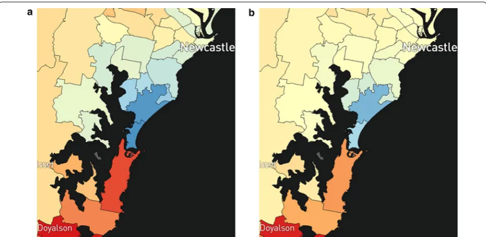
Transparency layer So that imprecise estimates do not give the impression of important differences, a second layer with varying degrees of opacity was also developed and displayed (Fig. 2). This has the pale-yellow colour of the Australian average in increasing opacity (0% if an estimate has a DPP of 1, 100% if an estimate has a DPP of 0), so that estimates with very high uncertainty were less visually distinguishable from the Australian average, regardless of their median values.
Graphs
Summary plots for large regions The nationwide pat-terns can be difficult to visualise geographically due to small SA2s, especially in urban areas, which are not visi-ble without zooming in. To overcome this, summary plots showing the distribution of SA2-specific estimates were developed so that all of Australia could be represented, either in its entirety (quintiles of area-based socioeco-nomic groups using the Index of Relative Socio-ecosocioeco-nomic Advantage and Disadvantage [53], remoteness areas (cat-egories of the physical distance of a location from the nearest areas of concentrated urban development with populations of 200 people or more) [54], or state and ter-ritory boundaries), or focused on regions which were dif-ficult to see on the map (greater capital city areas [55]). An example is shown in Fig. 3.
V‑plots A V-plot (Fig. 4) was developed as a new method for combing two pieces of information, namely the area-specific SIR/EHR estimates and the probability that these estimates are different from the Australian average. The x-axis compares the posterior median SIR/EHR of each area to the Australian average, while the y-axis is the pos-terior probability that the true incidence/relative survival for an area is different from the Australian average; this is given by the DPP. Estimates near the top of the V-plot are likely to reflect a real difference from the Australian average, while estimates near the bottom of the V-plot are unlikely to be a real difference.
the curve resulting from the non-linear intervals. Since these densities are not true densities, but are analogous in their interpretation, we refer to them as “wave plots”.
Results
The results of the statistical model and visualisation development were published through the release of the Australian Cancer Atlas (https ://atlas .cance r.org.au) in September, 2018. The Australian Cancer Atlas provides the first freely available, digital, interactive picture of cancer incidence and survival at the small geographi-cal level across Australia with a focus on incorporating uncertainty, while also providing the tools necessary for
Fig. 2 Partial map of liver cancer incidence for females with a transparency overlay disabled, and b transparency overlay enabled (default option)
Fig. 3 Example of the summary plots for large regions, showing liver cancer incidence for females by SA2 as a a percentage of SA2-specific estimates, and b a distribution (boxplot) of SA2-specific estimates
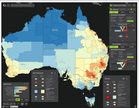
accurate estimation and appropriate interpretation and decision making. The main user interface of the Atlas is illustrated in Fig. 5.
Discussion
The Australian Cancer Atlas is the first comprehensive, interactive digital cancer atlas based on small areas and utilising spatial smoothing to describe geographical pat-terns of cancer incidence and survival across Australia. One of the key objectives of the Atlas was to motivate new research to gain a better understanding of why geo-graphical variation exists. Its success will be measured in part by how widely the Australian Cancer Atlas is used by key stakeholders, including members of the community, researchers, clinicians, and government, both as a source of information and to guide research and inform decision making.
Towards this aim, we plan an ongoing program of development and research. Future versions of the Atlas are planned to incorporate information about how geo-graphical patterns have changed over time, new indi-cators such as cancer screening, diagnostic tests, and cancer treatment, and alternative visualisations such as cartograms which alleviate overemphasis of spatial pat-terns exhibited by large but lesser populated areas.
It is also hoped that the Atlas will provide motivation and opportunity for a better understanding of why geo-graphical variation exists for each type of cancer. These investigations will need to consider in more detail the characteristics of people living within areas, the stage and other clinical characteristics of the cancer, treat-ment patterns, and the distribution of known cancer risk factors and cancer screening behaviour. They will also
incorporate ecological modelling to identify associations between key area-level factors and geographical patterns such as remoteness, area disadvantage and access to ser-vices. A multidisciplinary approach will be crucial to meet these goals, and it is hoped that the Atlas provides motivation and opportunity for different research groups to collaborate and combine existing data at the small area level.
Conclusions
Since its release in September 2018, the Australian Can-cer Atlas has brought new insights about geographical cancer patterns across Australia. It has already motivated new collaborations within Australia and internationally to better quantify and understand the geographical pat-terns of cancer indicators, and will continue to form the foundation of an ongoing research program incorporat-ing innovative statistical models and visualisations to better quantify the extent and characteristics of the geo-graphical variation, and the reasons why it exists.
Abbreviations
ACD: Australian Cancer Database; ASGS: Australian Statistical Geography Standard; CAR : conditional autoregressive; CrI: credible interval; DPP: differ-ence in posterior probabilities; EHR: excess hazard ratio; ICD: International Classification of Diseases; MCMC: Markov Chain Monte Carlo; MEET: Maximised Excess Events Test; SA2: Statistical Area 2; SIR: standardised incidence ratio.
Acknowledgements
The Research team acknowledge the support of the cancer registries within the Australasian Association of Cancer Registries in enabling this Cancer Atlas to proceed, and the guidance provided by members of the Project Advisory Group. The authors would also like to acknowledge the valuable contribution from the Visualisation and eResearch (ViseR) team, QUT, in developing the digital product and providing the expertise on technical matters.
Authors’ contributions
EWD, SMC conceptualisation, original preparation and revision of manuscript, visualisations; JFA conceptualisation, revision of manuscript; KLM conceptuali-sation, supervision, revision of manuscript; PDB conceptualiconceptuali-sation, supervision, original preparation and revision of manuscript. All authors read and approved the final manuscript.
Funding
The Australian Cancer Atlas is a collaborative study funded by the Fron-tierSI (formerly the Cooperative Research Centre for Spatial Information), Cancer Council Queensland, Australian Institute of Health and Welfare and Queensland University of Technology. The Atlas has additional support from the Centre for Research Excellence in Prostate Cancer Survivorship. It has been endorsed by the Australasian Association of Cancer Registries and Cancer Council Australia, and investigators access expertise from the Austral-ian Research Council Centre of Excellence for Mathematical and Statistical Frontiers (ACEMS).
Availability of data and materials
The datasets generated during the current study are available for download via the Australian Cancer Atlas (https ://atlas .cance r.org.au). The original data that support the findings of this study are available from the Australian Cancer Database, Australian Institute of Health and Welfare, but restrictions apply to the availability of these data, which were used under license for the current study, and so are not publicly available. With appropriate ethics and data custodian approvals, these data can be obtained from the Australian Institute of Health and Welfare.
Ethics approval and consent to participate
Ethical approval to undertake this study was obtained from research ethics committees in New South Wales (NSW) (NSW Population & Health Services Research Ethics Committee, Ref: 2017/HREC0203), Queensland (Queens-land University of Technology Human Research Ethics Committee, Ref. 1600000880), and the two territories (Australian Capital Territory (ACT) Health Human Research Ethics Committee, Ref. ETHLR.16.235 and Human Research Ethics Committee for the Northern Territory Department of Health and Men-zies School of Health Research, Ref: 2016-2720). Approval to extract the data was obtained from each State and Territory data custodian.
Consent for publication Not applicable.
Competing interests
The authors declare that they have no competing interests.
Author details
1 ARC Centre of Excellence for Mathematical and Statistical Frontiers, Queensland University of Technology (QUT), Brisbane, Australia. 2 School of Mathematics, Science and Engineering Faculty, Queensland University of Technology (QUT), Brisbane, Australia. 3 Cancer Council Queensland, PO Box 201, Spring Hill, Brisbane, QLD 4004, Australia. 4 Menzies Health Institute Queensland, Griffith University, Gold Coast, Australia. 5 School of Public Health, The University of Queensland, Brisbane, Australia. 6 School of Research-Public Health, Queensland University of Technology, Brisbane, Australia. 7 Institute for Resilient Regions, University of Southern Queensland, Brisbane, Australia.
Received: 17 April 2019 Accepted: 21 September 2019
References
1. Baade PD, Yu XQ, Smith DP, Dunn J, Chambers SK. Geographic disparities in prostate cancer outcomes—review of international patterns. Asian Pac J Cancer Prev. 2015;16(3):1259–75.
2. Dwyer-Lindgren L, Bertozzi-Villa A, Stubbs RW, Morozoff C, Mackenbach JP, van Lenthe FJ, et al. Inequalities in life expectancy among US counties, 1980 to 2014. JAMA Intern Med. 2017;177(7):1003–11.
3. Menigoz K, Nathan A, Heesch KC, Turrell G. Neighbourhood disadvan-tage, geographic remoteness and body mass index among immi-grants to Australia: a national cohort study 2006–2014. PLoS ONE. 2018;13(1):e0191729.
4. Padilla CM, Kihal-Talantikit W, Perez S, Deguen S. Use of geographic indicators of healthcare, environment and socioeconomic factors to char-acterize environmental health disparities. Environ Health. 2016;15(1):79. 5. Youl PH, Dasgupta P, Youlden D, Aitken JF, Garvey G, Zorbas H, et al. A
sys-tematic review of inequalities in psychosocial outcomes for women with breast cancer according to residential location and Indigenous status in Australia. Psychooncology. 2016;25(10):1157–67.
6. Public Health Information Development Unit. Social Health Atlas of Australia: Population Health Areas 2019. http://phidu .torre ns.edu.au/socia l-healt hatla ses/data#socia l-healt h-atlas -of-austr alia-popul ation -healt h-areas . Accessed 27 Sept 2019.
7. Australian Institute of Health and Welfare. Cancer incidence and mortality in Australia by small geographic areas, Cat. no. CAN 108; 2018. http:// www.aihw.gov.au/repor ts/cance r/cance r-incid ence-morta lity-small -geogr aphic -areas /data. Accessed 27 Sept 2019.
8. Small Area Health Statistics Unit. The Environment and Health Atlas of England and Wales. http://www.envhe altha tlas.co.uk/homep age/. Accessed 27 Sept 2019.
9. Geographic Information Systems and Science for Cancer Control, National Cancer Institute. National Cancer Atlas Application. 2019. https ://gis.cance r.gov/cance ratla s/app/. Accessed 27 Sept 2019.
11. Carlos III Institute of Health, National Center for Epidemiology. Interactive epidemiological information system (ARIADNA). http://ariad na.cne.iscii i.es/evind ex.html. Accessed 27 Sept 2019.
12. Cancer Council Queensland, Queensland University of Technology, Fron-tierSI. Australian Cancer Atlas. Version 09-2018. Brisbane: Cancer Council Queensland, QUT, FrontierSI. 2018. https ://atlas .cance r.org.au. Accessed 27 Sept 2019.
13. Australian Bureau of Statistics. Australian Statistical Geography Standard (ASGS): vol. 1. Main structure and greater capital city statistical areas. Canberra: ABS; 2011.
14. Australian Bureau of Statistics. Australian Statistical Geography Standard (ASGS): correspondences 2011, ‘Statistical Local Area 2011 to Statistical Area Level 2 2011’, data cube: Excel spreadsheet, cat. no. 1270.0.55.006; 2013www.abs.gov.au/AUSST ATS/[email protected]/Detai lsPag e/1270.0.55.006Ju ly%20201 1. Accessed 27 Sept 2019.
15. World Health Organization. International statistical classification of dis-eases and related health problems 10th Revision (ICD-10): 2016 version. Geneva: WHO; 2016.
16. Esteve J, Benhamou E, Raymond L. Statistical methods in cancer research volume IV: descriptive epidemiology. Lyon: International Agency for Research on Cancer; 1994.
17. Pickle LW. A history and critique of U.S. mortality atlases. Spat Spatiotem-poral Epidemiol. 2009;1(1):3–17.
18. Dickman PW, Adami HO. Interpreting trends in cancer patient survival. J Intern Med. 2006;260(2):103–17.
19. Brenner H, Hakulinen T. Up-to-date long-term survival curves of patients with cancer by period analysis. J Clin Oncol. 2002;20(3):826–32. 20. Australian Institute of Health and Welfare. Australian Cancer Database
Canberra: AIHW; 2018. https ://www.aihw.gov.au/about -our-data/our-datac ollec tions /austr alian -cance r-datab ase. Accessed 27 Sept 2019. 21. Australian Bureau of Statistics. ABS.Stat Dataset: ERP by Statistical Areas
Level 2 (SA2) geographical areas (ASGS 2011), age and sex, 2001 to 2016 ABS Cat No 3235.0. Australian Bureau of Statistics. Released August 2017. http://www.abs.gov.au/AUSST ATS/[email protected]/Detai lsPag e/3235.02016 . Accessed 27 Sept 2019.
22. Queensland Government. National death data 2018. https ://www.qld. gov.au/law/birth s-death s-marri ages-and-divor ces/data/natio nal-data. Accessed 27 Sept 2019.
23. Tobler W. A computer movie simulating urban growth in the Detroit region. Econ Geogr. 1970;46(2):234–40.
24. Hampton KH, Serre ML, Gesink DC, Pilcher CD, Miller WC. Adjusting for sampling variability in sparse data: geostatistical approaches to disease mapping. Int J Health Geogr. 2011;10(1):54.
25. Besag J. Spatial interaction and the statistical analysis of lattice systems. J R Stat Soc Ser B. 1974;36(2):192–225.
26. Banerjee S, Carlin BP, Gelfand AE. Hierarchical modeling and analysis for spatial data. 2nd ed. Boca Raton: Chapman and Hall/CRC; 2014. 27. Johnson GD. Small area mapping of prostate cancer incidence in New
York State (USA) using fully Bayesian hierarchical modelling. Int J Health Geogr. 2004;3(1):29.
28. Congdon P. Applied Bayesian hierarchical methods. London: Chapman and Hall/CRC Press; 2010.
29. Duncan EW, White NM, Mengersen K. Spatial smoothing in Bayesian models: a comparison of weights matrix specifications and their impact on inference. Int J Health Geogr. 2017;16(1):47.
30. Wall MM. A close look at the spatial structure implied by the CAR and SAR models. J Stat Plan Inference. 2004;121(2):311–24.
31. Best NG, Arnold RA, Thomas A, Waller LA, Conlon EM. Bayesian models for spatially correlated disease and exposure data. In: Bernardo JM, Berger JO, Dawid AP, Smith AFM, editors. Bayesian statistics 6: Proceedings of the sixth Valencia international meeting. Oxford: Oxford University Press; 1998. p. 131–56.
32. Earnest A, Morgan G, Mengersen K, Ryan L, Summerhayes R, Beard J. Evaluating the effect of neighbourhood weight matrices on smooth-ing properties of Conditional Autoregressive (CAR) models. Int J Health Geogr. 2007;6:54.
33. Conlon EM, Waller LA. Flexible neighborhood structures in hierarchical models for disease mapping. Report 1998–018. Minneapolis: University of Minnesota, Division of Biostatistics; 1998.
34. Rue H, Held L. Gaussian Markov random fields: theory and applications. Boca Raton: CRC Press; 2005.
35. Bell KP, Bockstael NE. Applying the generalized-moments estimation approach to spatial problems involving microlevel data. Rev Econ Stat. 2000;82(1):72–82.
36. Griffith DA. Some guidelines for specifying the geographic weights matrix contained in spatial statistical models. In: Arlinghaus SL, editor. Practical handbook of spatial statistics. Boca Raton: CRC Press; 1996. p. 65–82.
37. Cramb SM, Duncan EW, Baade PD, Mengersen KL. Investigation of Bayes-ian spatial models. Brisbane: Cancer Council Queensland and Queens-land University of Technology (QUT); 2017.
38. Leroux BG, Lei X, Breslow N. Estimation of disease rates in small areas: a new mixed model for spatial dependence. Stat Models Epidemiol Environ Clin Trials. 1999;116:179–91.
39. Besag J, York J, Mollié A. Bayesian image restoration with application in spatial statistics. Ann Inst Stat Math. 1991;43(1):1–20.
40. Best N, Richardson S, Thomson A. A comparison of Bayesian spatial mod-els for disease mapping. Stat Methods Med Res. 2005;14(1):35–59. 41. Fairley L, Forman D, West R, Manda S. Spatial variation in prostate cancer
survival in the Northern and Yorkshire region of England using Bayesian relative survival smoothing. Br J Cancer. 2008;99(11):1786–93. 42. Richardson S, Thomson A, Best N, Elliott P. Interpreting posterior relative
risk estimates in disease-mapping studies. Environ Health Perspect. 2004;112(9):1016–25.
43. Metropolis N, Rosenbluth AW, Rosenbluth MN, Teller AH, Teller E. Equa-tions of state calculaEqua-tions by fast computing machine. J Chem Phys. 1953;21(6):1087–92.
44. Rue H, Martino S, Chopin N. Approximate Bayesian inference for latent Gaussian models by using integrated nested Laplace approximations. J R Stat Soc Ser B. 2009;71(2):319–92.
45. R Core Team. R: a language and environment for statistical computing. Vienna: R Foundation for Statistical Computing; 2017.
46. Lee D. CARBayes: an R package for Bayesian spatial modeling with condi-tional autoregressive priors. J Stat Softw. 2013;55(13):1–24.
47. Lunn DJ, Thomas A, Best N, Spiegelhalter D. WinBUGS—a Bayesian modelling framework: concepts, structure, and extensibility. Stat Comput. 2000;10(4):325–37.
48. Sturtz S, Ligges U, Gelman A. R2WinBUGS: a package for running Win-BUGS from R. J Stat Softw. 2005;12(3):1–16.
49. Geweke J. Evaluating the accuracy of sampling-based approaches to the calculation of posterior moments. In: Bernardo JM, Berger J, Dawid AP, Smith AFM, editors. Bayesian statistics 4. Oxford: Oxford University Press; 1992. p. 169–93.
50. Tango T. A test for spatial disease clustering adjusted for multiple testing. Stat Med. 2000;19(2):191–204.
51. Kulldorff M, Song C, Gregorio D, Samociuk H, DeChello L. Cancer map patterns: are they random or not? Am J Prev Med. 2006;30(2):S37–49. 52. Cramb S, Mengersen L, Baade P. Developing the atlas of cancer in
Queensland. Int J Health Geogr. 2011;10:9.
53. Australian Bureau of Statistics. Census of Population and Housing: Socio-Economic Indexes for Areas (SEIFA), Australia, 2011. Canberra: ABS; 2013. 54. Australian Bureau of Statistics. Australian Statistical Geography Standard
(ASGS): volume 5—remoteness structure, 2011. Canberra: ABS; 2013. 55. Australian Statistical Geography Standard (ASGS): volume 1—main
structure and greater capital city statistical areas, July 2011: cat. no. 1270.0.55.001; 2011. https ://www.abs.gov.au/AUSST ATS/[email protected]/Detai lsPag e/1270.0.55.001Ju ly%20201 1. Accessed 27 Sept 2019.
Publisher’s Note