M. Belhaq, P. Lafitte and T. Leli`evre Editors
ASYMPTOTIC METHOD FOR TRULY NON-LINEAR OSCILLATOR WITH
TIME VARIABLE PARAMETER
Livija Cveticanin
1Abstract. In this paper a new analytical method for solving the truly (pure) non-linear differential equation with slow-time variable parameter is developed. The method is based on the solution of the corresponding differential equation with a constant parameter, where the exact frequency of vibration is introduced. The approximate solution of the differential equation with time variable parameter is assumed in the aforementioned form, but with time variable amplitude and phase. The solution of the differential equation is nonstationary with time variable amplitude and period of vibration. In the paper an example with linear time variable parameter and non-integer order non-linearity is considered. The obtained approximate solution of the differential equation is compared with an exact numerical one and shows good agreement.
1.
Introduction
In a lot of machines, such as centrifuges, transportation equipment, dozers, melting pots, etc., the mass of the system is time-varying. Most of these machines are applied in the process industry and work under special conditions (high temperature, corrosion, high pressure). Very often the built-in material is not steel but copper, aluminium or its alloys, ceramic material, plastic, etc. Experimental investigation of elastic properties for a significant number of materials applied in contemporary mechanical and civil engineering give the nonlinear strain-stress relation with the order which is of integer or noninteger type (see for example [1] - [4]). The question is how these elastic properties of the materials affect the motion of the system. Some investigations have already been done. For example, in papers [5] and [6] the bending of a beam made of nonlinear material is considered. Haslach investigated the post-buckling behavior of the column made of wood [7] and also of the beam made of polymers with nonlinear elastic properties [8]. The vibrations of a composite material beam [9] and of the piano hammer made of a wooden beam, which is coated with several layers of compressed wool felts [10], were also analyzed. In paper [11], vibrations in the vehicle under influence of the suspension and the tires are considered. The open celled polyurethane foam automotive seat cushions [12]- [13] are described as nonlinear vibration models. The nonlinear vibrations of the micro-oscillators [14], micro-filters [15], micro-actuators [16], etc., affected by nonlinearity of the restitution force are treated. Finally, in all of the mentioned problems it is evident that the existence of the nonlinear elastic property has an influence on motion, especially on the vibration of a system with constant parameters.
In this paper the influence of the nonlinear elastic force on the vibration of the parameter variable system is investigated. Namely, the interaction between the nonlinear elastic property and the parameter variation on the vibration of the one-degree-of-freedom oscillator is considered. In general, the mathematical model of a truly
1 Faculty of Technical Sciences, University of Novi Sad,
Trg D. Obradovica 6, 21000 Novi Sad, Serbia
c
EDP Sciences, SMAI 2013
(pure) nonlinear oscillator with time variable parameter is described as
¨
x+c21(εt)x|x|α−1= 0, x(0) =A0, x(0) = 0.˙ (1)
where α is the order of nonlinearity, c21(εt)≡ c21(τ) is the time variable function,A0 is the initial amplitude. Let us assume that the parameter variation is slow and is a function of the slow timeτ =εt whereε <<1 is a small parameter. The order of nonlinearityαis obtained experimentally and is in general a positive rational number :α∈Q+.
The investigations are most often directed toward the linear oscillator (α= 1), which represents a special case of (1), i.e.,
¨
x+c21(εt)x= 0, x(0) =A0, x(0) = 0˙ (2) Various asymptotic methods are developed for solving the linear second order differential equation with time-variable parameter (2). The most often applied are the method of multiple scales [17], method of averaging [18], method of variable amplitude and phase [19], method of harmonic balance [20], etc. The aforementioned methods are applied for solving the special problem of vibrations of oscillators with variable mass (see for example [21]-[26]) which are applied in techniques and engineering. Yuste [27] was the first to consider the oscillator with time-variable parameter, but also with a strong nonlinear term of the third order
¨
x+c21(εt)x3= 0, x(0) =A0, x(0) = 0.˙ (3) Based on the exact solution of the pure cubic nonlinear oscillator with constant parameterc2
1(0) :
¨
x+c21(0)x3= 0 (4)
the asymptotic analytical solution of (3) is assumed in the form of a Jacobi elliptic function with time variable amplitude and phase. The approximate solution of (3) is considered in the form of the cosine trigonometric function by Cveticanin [23]. The approximate solution is assumed with time variable amplitude and phase, but also time variable frequency. Comparing the approximate solution based on the Jacobi elliptic function (see [27]) with the solution based on the trigonometric function (see [23]) for (3), it is evident that the first result is better. The accuracy of solution depends on how well (4) approximates to (3).
Based on the aforementioned method, in this paper, a procedure for solving of the truly nonlinear oscillator with time-variable parameter is developed. Assuming that (1) approximates to the differential equation with constant parameter
¨
x+c21(0)x|x|α−1= 0 (5) with high accuracy, the solution of (5) is determined. In the paper [28] the exact solution in the form of A-teb function [29]- [31] of the differential equation (5) is determined. To introduce the perturbation to this solution is very complex and very inconvenient for further application for engineers. It is the reason, that in this paper the approximate cosine solution for (5) is used as the basic one for solving the differential equation (1)
x=A0cos(ω0t+θ) (6)
whereAandθare arbitrary constants which depend on the initial conditions andω0is the frequency of vibration. It is important to mention that the exact value of the frequency i.e. period of vibration for (5) can be calculated analytically. Namely, the first integral for (5) with initial conditions (1) is
˙ x2
2 +c 2 1(0)
|x|α+1
α+ 1 =c 2 1(0)
Aα+10
α+ 1. (7)
After some transformation of (7) and integration, the exact period, i.e., frequency of vibration for (5) is obtained as (see [32])
ω0=|A0| (α−1)/2
q
q
c2
with
q=
r
α+ 1 2
√
πΓ(2(α+1)3+α )
Γ( 1 α+1)
(9)
where Γ is the gamma function [33]. The frequency (8) is substituted into (6) and the solution approximately satisfies the differential equation (5), i.e.,
−A0ω20cos(ω0t+θ) +c21(0)|A0| α
cos(ω0t+θ)|cos(ω0t+θ)| α−1
≈0. (10)
The solution (6) with the exact frequency of vibration (8) has the advantage that the period of vibration is constant during the whole working interval. Based on the solution in the first period the prediction of the motion for any period of vibration is possible. It is due to the fact that the motion during all of the periods of vibration is equal. Then, x(0) = x(T1) =x(T2) =...=x(Tn) =x(T) =A =const.and there is no error accumulation during the whole working period. Analyzing the relation (8) it is evident that the angular frequency of vibration depends on the order of nonlinearity α,but also on the initial amplitudeA and the coefficient of nonlinearity c2
1(0).
This paper is divided into four Sections. After the Introduction, in Section 2 the solution procedure for (1) based on (6) with (8) is developed. The well known averaging method is used for an approximate solution (see Section 3). In Section 4, the obtained results are applied for a truly nonlinear oscillator with linear time-variable parameter. The approximate solution for the differential equation is calculated and compared with a numerical one. The paper ends with the Conclusion.
2.
Solution procedure
Let us assume the trial solution of (1)and its first time derivative in the form of the generating solution (6) and its first time derivative, but with time-variable amplitudeA(t), phaseθ(t) and frequencyω(A, τ)≡ω(A(t), τ)
x=A(t) cosψ(t) (11)
and
˙
x=−A(t)ω(A, τ) sinψ(t) (12) with
ψ(t) =
Z t
0
ω(A(s), εs)ds+θ(t) (13)
The calculated first time derivative of (11) is
˙
x=−A(t)ω(A, τ) sinψ(t) + ˙A(t) cosψ(t)−A(t) ˙θ(t) sinψ(t). (14)
Comparing (12) and (14) it is
˙
A(t) cosψ(t)−A(t) ˙θ(t) sinψ(t) = 0 (15)
Substituting (11) and the time derivative of (12) into (1) we obtain
−d
dt(Aω) sinψ−Aω ˙
θcosψ−Aω2cosψ+c21|A|αcosψ|cosψ|α−1= 0 (16)
whereA≡A(t), θ≡θ(t), ψ≡ψ(t) and according to (8)
ω≡ω(A, τ) =|A(t)|(α−1)/2q
q
c2
1(τ). (17)
Using the relation (10), the sum of the last two terms on the left side of the equation (16) is approximately zero,
and
−d
dt(Aω) sinψ−Aω ˙
θcosψ= 0 (19)
After some modification of (15) and (19), the differential equation (1) is rewritten into two first order differential equations
Aθ(ω˙ +A∂ω ∂Asin
2ψ) = −εA∂ω
∂τ sinψcosψ (20)
˙
A(ω+A∂ω ∂Asin
2
ψ) = −εA∂ω ∂τ sin
2
ψ (21)
Our task is to determine the functions A(t) and θ(t) which satisfy the equations (20) and (21). To obtain the exact analytical solutionsA(t) andθ(t) is not an easy task. It is at this point that the averaging over the period of vibration is introduced.
3.
Averaging procedure
Using the periodical property of the trigonometric functions sinψ and cosψ, the averaging of the differential equations of motion (20) and (21) over the period of 2πis done (see [34])
Aθ˙
ω+A∂ω ∂A
1 2π
Z 2π
0
sin2ψdψ
= −εA∂ω ∂τ
1 2π
Z 2π
0
sinψcosψdψ (22)
˙ A
ω+A∂ω ∂A
1 2π
Z 2π
0
sin2ψdψ
= −εA∂ω ∂τ
1 2π
Z 2π
0
sin2ψdψ (23)
After integration, the obtained averaged differential equations of motion are
˙ A
ω+1 2A
∂ω ∂A
= −εA1 2
∂ω
∂τ (24)
Aθ˙
ω+1 2A
∂ω ∂A
= 0 (25)
The averaged equations (24) and (25) can be rewritten as
˙ A A =−
1 2 ˙ ω ω, ˙
θ= 0 (26)
Integrating the differential equations (26) and using the initial amplitude A0, initial frequency ω0 and initial phase angleθ(0),we obtain the averaged amplitude
A A0 =
r
ω0
ω , θ=θ(0) (27)
i.e.,
A=A0
p
c2 1(0)
p
c2 1(τ)
!α2+3
(28)
and phase angle
ψ=ω0
Z t 0 p c2 1(τ) p c2 1(0)
!α+34
Substituting (28) and (29) into (11) the averaged approximate solution is
x=A0
p
c2 1(0)
p
c2 1(τ)
!α2+3
cos(ω0
Z t
0
p
c2 1(τ)
p
c2 1(0)
!α+34
dt+θ(0)) (30)
Analyzing the relations (28) and (29) it is obvious that both, the amplitude and frequency of vibration, depend on the time-variable coefficient and on the order of nonlinearity. The averaged amplitude is the product of the initial amplitudeA0 and of a time variable function : ifc21(τ) is an increasing function,the amplitude decreases and the amplitude increases if the functionc21(τ) decreases in time.
According to the assumption (12) and the solution (30), the approximate velocity of vibration is
˙
x=−A0ω0
p
c2 1(τ)
p
c2 1(0)
!α+32
sin(ω0
Z t
0
p
c2 1(τ)
p
c2 1(0)
!α+34
dt+θ(0)) (31)
It can be seen that the velocity of vibration increases by increasing the functionc2
1(τ) in time, and decreases if the functionc21(τ) decreases in time.
4.
Example
Let us consider an example where the parameter variation is a linear time function, i.e., c1 = (1 +εt) and the order of nonlinearity isα= 5/3.Mathematical model of the oscillator is
¨
x+ (1 +εt)2x|x|2/3= 0 (32)
and the initial conditions are assumed as
x(0) =A0= 1, x(0) = 0˙ (33)
Using the aforementioned solution procedure, the approximate analytical solution is
x= A0
(1 +εt)3/7cos( 0.50659
ε A 1/3
0 ((1 +εt)
13/7−1)) (34)
where the amplitude variation is
A=± A0
(1 +εt)3/7. (35)
The approximate velocity of vibration function of the oscillator (32) is due to (31)
˙
x= 0.94081A4/30 (1 +εt)3/7sin(0.50659 ε A
1/3
0 ((1 +εt)
13/7−1)) (36)
The differential equation (32) is also solved numerically, by applying the Runge-Kutta solution procedure. Three various values of the small parameterε are introduced into calculation. The time considered for the oscillators isε−1.
(i) For the oscillator whereε= 0.1 the corresponding analytical solution and its time derivative are
x= (1 + 0.1t)−3/7cos(5.0659((1 + 0.1t)13/7−1)) (37)
˙
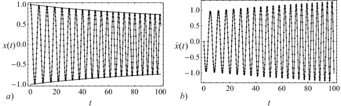
Figure 1. (a)x−t diagrams obtained analytically (full line) and numerically (dot line), and envelope curvesA−t; (b) ˙x−tdiagrams obtained analytically (full line) and numerically (dot line) forε= 0.1.
In Fig.1.a, we plotted thex−t diagrams obtained numerically and analytically according to (37) and also the amplitude envelope curves
A=±(1 + 0.1t)−3/7 (39)
It can be seen that the envelope curves are on the top of the numeric solution. The amplitude and the period of vibration decrease in time. Comparing the analytical and numerical results, it is obvious that the difference between them is negligible even for a long time period (2ε−1).
In Fig.1b the ˙x−tdiagrams obtained analytically and numerically are plotted. An excellent agreement for the periods of vibration is evident.
(ii) If the parameter of the oscillator isε= 0.01,the motion of the oscillator is
x= (1 + 0.01t)−3/7cos(50.659((1 + 0.01t)13/7−1)), (40)
with amplitude
A=±(1 + 0.01t)−3/7 (41)
and the velocity of vibration
˙
x= 0.94081(1 + 0.01t)3/7sin(50.659((1 + 0.01t)13/7−1)) (42)
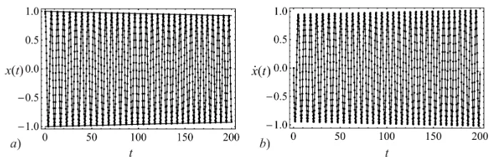
In Fig.2 we plot thex−tand ˙x−tdiagrams obtained numerically and analytically and also the envelope curve A−t. The considered time is 1/ε = 100. The curves are in good agreement in spite of long time motion.
Figure 3. a) x−t diagrams obtained analytically (full line) and numerically (dot line), and envelope curvesA−t; b) ˙x−tdiagrams obtained analytically (full line) and numerically (dot line) forε= 0.001.
(iii) In Fig.3, forε= 0.001 thex−tdiagram
x= (1 + 0.001t)−3/7cos(506.59((1 + 0.001t)13/7−1)) (43)
theA−t
A=±(1 + 0.001t)−3/7 (44)
and the ˙x−tdiagram
˙
x= 0.94081(1 + 0.001t)3/7sin(506.59((1 + 0.001t)13/7−1)) (45)
are compared with corresponding numerical ones. Due to inconvenience of long time presentation, the diagrams are plotted in the time period up to 200, which represents the value 0.2ε−1.A good agreement between the results is evident.
Remark : The mathematical model (32) corresponds to a mass variable system where the reactive force is zero. The mass slowly decreases in time and is given asm(τ) = (1 +εt)−2. In cases when the relative velocity of mass variation is zero, the reactive force is also zero.
5.
Conclusion
The following is concluded :
1. The vibration of the truly (pure) nonlinear oscillator with slow-time variable parameter is nonstationary, i.e., with time variable amplitude and phase. The correction of the initial amplitude is due to parameter variation and with the order which corresponds to the nonlinearity of the system. The same is valid for the phase variation. 2. The method suggested in the paper, which is based on the exact frequency of vibration of the correspond-ing oscillator with constant parameter gives very accurate results in comparison with the numerical solutions obtained by solving the truly (pure) nonlinear differential equation with slow-time variable parameter. The asymptotic solution is valid for the long time period.
Acknowledgement
References
[1] S.I. Dymnikov,Issues on Dynamics and Strength,No.24, 163-173 (1972) (in Russian).
[2] C.F. Beards,Engineering vibration analysis with application to control systems, London, Edward Arnold (1995). [3] E.I. Rivin,Passive vibration isolation, New York, Asme Press (2003).
[4] Aeroflex International, www.vmc-kdc.com (Accessed 15 July 2009).
[5] C.C. Lo, S.D. Gupta,Bending of a nonlinear rectangular beam in large deflection, Journal of Applied Mechanics 45, 213-215 (1978).
[6] G. Lewis, F. Monasa,Large deflections of cantilever beams of non-linear material of the Ludwick type subjected to an end moment, International Journal of Non-Linear Mechanics 17, 1-6 (1982).
[7] H.W. Haslach,Post-buckling behavior of columns with non-linear constitutive equations, Int. J. Non-Linear Mechanics 20, 53-67 (1982).
[8] H.W. Haslach,Influence of adsorbed moisture on the elastic post-buckling behavior of columns made of non-linear hydrophilic polymers, Int. J. Non-Linear Mechanics 27, 527-546 (1992).
[9] W-H. Chen, R.F. Gibson,Property distribution for nonuniform composite beams from vibration response measurements and Galerkin’s method, Journal of Applied Mechanics 65, 127-133 (1988).
[10] D. Russell, T. Rossing,Testing the nonlinearity of piano hammers using residual shock spectra, Acustica - Acta Acustica 84, 967-975 (1998).
[11] Q. Zhu, M. Ishitoby,Chaos and bifurcations in a nonlinear vehicle model, Journal of Sound and Vibration 275, 1136-1146 (2004).
[12] W.N. Patten, S. Sha, C. Mo,A vibration model of open celled polyurethane foam automative seat cushions,Journal of Sound and Vibration 217, 145-161 (1998).
[13] C.V. Jutte,Generalized synthesis methodology of nonlinear springs for prescribed load - Displacement Functions, Ph.D. Dis-sertation, Mechanical Engineering, The University of Michigan (2008).
[14] J.F. Rhoads,Generalized parametric resonance in electrostatically actuated micromechanical oscillators, Journal of Sound and Vibration 296, 797-829 (2006).
[15] J.F. Rhoads, Tunable micromechanical filters that exploit parametric resonance, Journal of Vibration and Acoustics 127, 423-430 (2005).
[16] C. Cortopassi, O. Englander, Nonlinear springs for increasing the maximum stable deflection of MEMS Electrostatic gap closing actuators, UC Berkeley, http ://robotics.eecs.berkeley.edu/˜pister/245/project/CortopassiEnglander, On 10th March (2009).
[17] A.H. Nayfeh, D.T. Mook,Nonlinear oscillations, Wiley, New York (1979).
[18] N.N. Bogolyubov, Ju.A. Mitropolski,Asimptoticheskie metodi v teorii nelinejnih kolebanij, Nauka, Moscow (1974). [19] N. Krylov, N. Bogolubov,Introduction to nonlinear mechanics,Princeton University Press, Princeton, New Jersey (1943). [20] L. Cveticanin,Approximate solution of a time-dependent differential equation, Meccanica 30, 665-671 (1995).
[21] A.P. Bessonov,Osnovji dinamiki mehanizmov s peremennoj massji zvenjev, Nauka, Moscow (1967).
[22] P.G.L. Leach,Harmonic oscillator with variable mass, Journal of Physics A : General Physics 16, No.14, 3261-3269., art.no. 019 (1983).
[23] L. Cveticanin,The influence of the reactive force on a nonlinear oscillator with variable parameter, Trans. ASME, J. of Vibrat. and Acoustics 114, No. 4, 578-580 (1992).
[24] L. Cveticanin,Dynamics of machines with variable mass, Gordon and Breach Science Publishers, London (1998). [25] J. Flores, G. Solovey, S. Gill,Variable mass oscillator, American Journa of Physics 71, No. 7, 721-725 (2003).
[26] L. Cveticanin, I. Kovacic,On the dynamics of bodies with continual mass variation, Trans ASME, Journal of Applied Mechanics 74, 810-815 (2007).
[27] S. Bravo Yuste,On Duffing oscillators with slowly varying parameters, Int. J Non-Linear Mech. 26, No. 5, 671-677 (1991). [28] L. Cveticanin, T. Pogany, Oscillator with a sum of non-integer order non-linearities, Journal of Applied Mathematics,
doi :10.1155/2012/649050, art. no. 649050, 20 pages, (2012).
[29] R. Rosenberg,The Ateb(h)-functions and their properties, Quart. Appl. Math. 21, No.1, 37-47 (1963).
[30] H.T. Drogomirecka,On integration of a special Ateb-function, Visnik Lvivskogo Universitetu, Serija mehaniko-matematichna 46,108-110 (1997) (in Ukranian).
[31] V.V. Gricik, M.A. Nazarkevich,Mathematical models algorythms and computation of Ateb-functions, Dopovidi NAN Ukraini Ser. A 12, 37-43 (2007) (in Ukranian).
[32] L. Cveticanin,Oscillator with fraction order restoring force, J. Sound and Vibration 320, No.4-5, 1064-1077 (2009).
[33] M. Abramowitz, I.A. Stegun,Handbook of mathematical functions with formulas, graphs and mathematical tables, Nauka, Moscow (1979) (in Russian).