Modeling the Container Selection for Freight
Transportation: Case Study of Iran
Seyed Sina Mohri1, Hossein Haghshenas2
Received: 09.03. 2016 Accepted: 06. 02. 2017
Abstract
Significant advantages of intermodal and containerized transport have increased the global interest to this mode of transportation. This growing interest is reflected in the annual volume of container cargo growth. However, the container transport inside Iran does not have a proper place. Comparing the count of containers entering and leaving ports with the statistics obtained from railway and road maintenance organizations showed that more than 77% of the containerized imports have been stripped at ports and dispatched toward their ultimate destinations outside containers. These statistics also showed that more than 81% of the containerized exports have transported to ports by means other than containers. The main purpose of this study was to identify the most important variables affecting the selection of containerized freight transport and non-containerized freight transport options by applying decision tree models on the road freight movement and a set of variables describes the differences between these two options. The final model representing the selection of containerized transport was developed by the use of CHAID, QUEST, C5 and C$R decision tree algorithms. The results showed that the decision tree built via pruned C5 algorithm provides the best accuracy and most sensible list of important parameters. High-value and perishable commodities showed the greatest potential for containerized transport. The most important policy factors that could affect the tendency of cargo owners to use containerized transport are tariffs and the status of destination (whether it is a port). Policies that could encourage cargo owners to use intermodal transport include setting a lower tariff on container handling, reducing the cost of loading and unloading, increasing the port facilities supporting the containerized transport, adjusting customs, and development of dry ports.
Keywords: Container, freight transport, decision tree, port, tariff
Corresponding author E-mail: [email protected]
1MSc Student, Department of Transportation Engineering, Isfahan University of Technology, Isfahan, Iran 2Assistant Professor, Department of Transportation Engineering, Isfahan University of Technology, Isfahan,
Modeling the Container Selection for Freight Transportation: Case Study of Iran
1. Introduction
The combined transport has merged the advantages of naval, rail and road transport by changing the structure of both vehicle and packaging to facilitate the use of intermodal containers, which in turn has reduced the costs and time and increased the safety and ease of freight transportation. The intermodal transport is a general variant of combined transport that plays a vital role in global and international trade. Significant advantages of intermodal and containerized transport have increased the global interest to this mode of transportation. This growing interest is reflected in the fact that, as Figure (1-a) shows, the volume of intermodal transport has increased from 299 million TEU in 2003 to 602 million TEU in 2012 [Degerland, 2011]. However, as Figure (1-b) shows, the increase in Iran’s intermodal freight transport during the same period has been minimal [UNCTAD, 2012]. According to statistics of road and railroad transport authorities, in 2013, the intermodal containers have been the means of only 6.5 million tons of freight, namely 1.6 percent of Iran’s total
domestic freight transport [Mohri and
Haghshenas, 2015]. Meanwhile, the Persian Gulf countries like United Arab Emirates, Saudi Arabia and Oman has had a better performance in this regard. Several studies have studied the containerized transport to model the selection of transit mode [Ortuzar, and Palma, 1988]. Winston has studied the transit of household goods and the use of containers as the vessels of transportation in coastal corridors [Winston, 1981b]. Viera has incorporated the intermodal transport as an option in his selection models. Due to lack of sufficient information, this study has considered the average cost and time of road and railroad based containerized transport to be equal to average cost and time pertaining to transport of all goods in these systems. This study has also failed to provide convincing reasons regarding the separation of rail and road systems [Vieira,
1992]. Fuchs et al. have used the LAPP method to model the domestic developments of intermodal freight transport from Great Britain to continental Europe [Fowkes, Nash, and Twedle, 1991]. A similar methodology has also been used by Shingal and Fuchs (2006) to study the same subject in India [Shinghal, and Fowkes, 2002]. Ravibabu has considered three modes of intermodal transport - railroad, road and bulk - and has used the nested logit model to model the transport of exports in Delhi-Mumbai corridor [Ravibabu, 2013]. In recent years, several researchers have compared the efficiency of data mining models with logit and probit models. Abdul Wahab and Sayyed have compared the efficiency of neural network model in vehicle selection (truck or train) with that of logit and probit models. Their study has reported that neural network models are as
efficient as logit and probit models
purpose of this study was to identify the most important variables affecting the selection of containerized freight transport and non-containerized freight transport options by applying decision tree models on the road freight movement and a set of variables describes the differences between these two options. The product owners by assessing various factors such as Costs of containerized transport (including shipping cost, demurrage costs, the cost of returning empty containers, etc.), Costs of non-containerized transport, the lack of empty containers and existing facilities at origin and destination, select one of the
containerized transport and non-containerized transport options. Therefore, in this study a set of the most important differences between these two options have been identified and some appropriate variables have been defined. One of the most widely used methods in modeling the decision problem, is using decision tree. Therefore by using decision tree, the most important variables affecting the choice of container in the country have been identified and some recommendations have been to strengthen the container transport in Iran has been proposed.
Figure 1. The volume of global intermodal transport during 2003-2012
2. Raw Data
The sources of statistical data collected for analysis and modeling are shown in Table 1. The data regarding Iran’s intermodal transport were collected through a variety of procedures from Iran’s road maintenance organizations, railway organization, customs administration, and shipping and ports organization. Iran’s shipping and ports organization publishes an annual report containing the statistics regarding all containers entered or left the country. Iran’s road maintenance organizations and railway organization issue separate bills of lading for transport of containerized cargo between ports and inland destinations. Transportation of containerized cargo in Iran can be classified into three categories: exports, imports and
domestic transit. Import and export of containerized cargo through land borders are only recorded via international bills of lading issued by either road maintenance organization or railway organization, and import and export of containerized cargo through maritime borders are recorded via domestic bills of lading [Mohri and Haghshenas, 2015]. According to statistics of Road Maintenance
and Railway Organization, in 2013,
containerized cargo constituted only 1.6 percent of Iran’s total internal freight transport and the total quantity of containerized freight transported via roads and railroads were limited to about 6.5 million tons.
Comparing the data of road maintenance
299
351 383 433
484 509 472
541 580 602
00 100 200 300 400 500 600 700
2003 2004 2005 2006 2007 2008 2009 2010 2011 2012
mi
lion
TE
U
Figure (1-b)
0 2 4 6 8 10 12 14 16 18 20
2005 2006 2007 2008 2009 2010 2011 2012
mi
lion TE
U
year
Figure (1-a)
OMN
IRN
KWT
BHR
ARE
SAU
PAK
Modeling the Container Selection for Freight Transportation: Case Study of Iran
organization, railway organization, and
shipping and ports organization showed that containerized freights transported toward the ports constitute only 19 percent of total containerized exports, and only 23 percent of cargos imported in containers proceeded to inland destinations within the same form. Table 3 shows the details of this information.
The reason behind the mismatch between data of road maintenance and railway organizations and that of shipping and ports organization regarding containerized exports is the lack of containerization at the primary source; this means that cargos to be exported are often transferred to ports by means other than modal containers, and there they must be reloaded for shipment. In the case of containerized imports,
the mismatch between data of road
maintenance and railway organization and that of shipping and ports organization can be attributed to a process known as stripping of containers. For several reasons, the owners of cargo tend to strip the imported containers and reload the goods to normal trucks, which then haul the cargo to all inland destinations. As Table 2 shows, more than 92 percent of containerized cargos were transported via
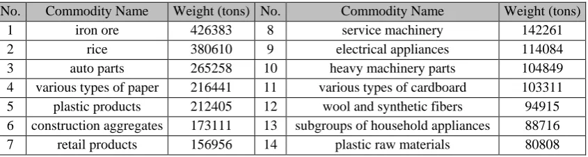
roads, so the data pertaining to domestic bills of lading issued by road maintenance organization was used as the basis of modeling. Moreover, the data collected from railway organization lacked packaging codes and only mentioned the name of containers in the column specifying the cargo type. The data collected from other organizations were used to check the accuracy of primary data and to prepare other variables of the model. The data of road maintenance organization included origin, destination, type of cargo, type of packaging, transportation tariffs, etc. As Table 4 shows, the major containerized cargos included commodities such as iron ore, rice, auto parts, various types of paper, and plastic products.
To model the selection of containerized
transport for road-based transportations,
commodities were divided into two categories: highly containerizeable commodities, and
non-containerizeable commodities. Highly
containerizeable commodities are those that were transported by containers, or those whose origin and destination had a record showing the transport of more than 100 tons of that commodity in containerized form.
Table 1. The raw data used in the study
Source Data
Road Maintenance Organization
bills of lading and corresponding packaging codes issued during 2013 and 2014
Railway
Organization bills of lading issued during 2013 and 2014 Road Maintenance
Organization import, export, and transit statistics for years 2013 and 2014 Customs
Administration
Statistics concerning the temporary entry of containers for years 2013 and 2014
Customs Administration
import and export statistics of different customs offices, plus the method used abroad for transport
Shipping And Ports Organization
Table 2. The overall quantity of containerized cargo transported via roads and railroads
Year Mode of transport
Cargo transported via containers (million tons)
Total cargo transported (million tons)
The share of containerized cargo in total
transport
The share of method of transport in total
containerized transport 201
3 Road 6.07 380.93 1.6 percent 92 percent
201
3 Railroad 0.52 30.26 1.7 percent 8 percent
Table 3. The volume of containerized cargo transported via roads and railroads to/from ports in comparison with volume of containerized imports and exports
Year Category
containerized cargo transported via roads and railroads to/from ports
(million tons)
containerized imports and exports
(million ton)
The share of intermodal
transport
2013 imports 2.7 11.5 23%
2013 exports 1.5 7.7 19%
Table 4. The major containerized cargos transported in Iran
No. Commodity Name Weight (tons) No. Commodity Name Weight (tons)
1 iron ore 426383 8 service machinery 142261
2 rice 380610 9 electrical appliances 114084
3 auto parts 265258 10 heavy machinery parts 104849 4 various types of paper 216441 11 various types of cardboard 103311 5 plastic products 212405 12 wool and synthetic fibers 94915 6 construction aggregates 173111 13 subgroups of household appliances 88716 7 retail products 156956 14 plastic raw materials 80808
3. Decision Tree Classification
The widely-known classification techniques include decision trees, Bayesian classifiers, conditional classifiers, SVM algorithms,
similarity-based classifiers, regression
methods, genetic and fuzzy algorithms, and neural networks, but this study used the decision tree classification for it adjustability and accuracy [Esmaeili, 2014]. Decision Trees are a form of data mining models that can be used as classifiers and regression finders. As their name implies, each decision tree is made up of a number of nodes and branches. In a classifier tree, each leaf represents a class, and other nodes (non-leaf nodes) represent one or more decision-specific attributes.
3.1 Attribute selection criteria
The attribute selection criteria considered for building the decision tree are briefly introduced below:
3.1.1 Information Gain:
Information Gain is one of the best-known measures commonly used for building decision trees. This measure is itself based on another factor called entropy.
( 1 ) Information Gain(A)
= Entropy(D) − EntropyA(D)
In this formula, which calculates the information gain of attribute A, D denotes the data set, and:
( 2 ) Entropy(D) = − ∑ Pi× log2(Pi) d
c
Modeling the Container Selection for Freight Transportation: Case Study of Iran
( 3 ) EntropyA(D)
= − ∑|D|D|j|× Entropy(Dj) d v
j=1
In the above formulas, C denotes the number of
class labels in dataset, Pi is the probability of a
sample belonging to the class i, V denotes the number of members in the domain of attribute
A, and Dj represents that part of the primary
data whose attribute has the value Vj. Also, |D|
denotes the size of the dataset D.
3.1.2 GINI Index
The GINI Index of dataset D could be calculated via the following formula.
(4) Gini(D) = 1 − ∑ Pi2
c
i=1
where C is the number of classes in dataset, and
Pi is the probability of a sample belonging to the
class i. For each attribute, this index injects a binary split into the tree. When dataset D is divided (with respect to attribute A) into two
subsets D1 and D2, we have:
(5) GiniA(D) =
|D1|
|D| ∗ Gini(D1) + |D2|
|D| ∗ Gini(D2)
All states of binary classification must be considered for all attributes and after calculating the Gini index for all states, the minimum obtained value must be selected. In other words, ultimately the attribute with the lowest Gini index will be selected for the current node of decision tree. We can also select the attribute that maximizes the degree of impurity; this parameter can be calculated via the following formula:
(6) Gini(A) = Gini(A) − GiniA(D)
3.1.3 Gain Ratio
Gain Ratio, which in fact normalizes the information gain, is expressed as follows:
(7) GainRatioA(D)
=InformationGain (A) EntropyA(D)
When the denominator of above formula is
zero, this criterion is not definable. Previous measures are skewed toward attributes with greater domains. In other words, these measures will always favor the attributes with greater values over those with lower values. So it seems that a measure should normalize these criteria. It can be shown that the use of Gain Ratio provides model with levels of accuracy and sophistication surpassing those provided by Information Gain. The problem associated with the use of this measure is the manner of finding breakpoints for continuous (numerical) datasets with large number of distinct values; however the same weakness can also be attributed to information gain. The other attribute selection criteria include Likelihood Ratio and DKM.
3.2 Decision Tree Algorithms
There are several algorithms for building decision trees, the most important of which are discussed below.
3.2.1 ID3 Algorithm
ID3 is one of the simplest decision tree algorithms that use information gain as selection criteria. This algorithm has two termination conditions: i) the remaining samples all belong to a single class, and ii) the highest calculated information gain is not greater than zero. This algorithm does not utilize any pruning technique and can accept numeric attributes and incomplete data as input [Esmaeili, 2014].
3.2.2 CART Algorithm
This algorithm produces a binary decision tree, where each internal node has exactly two branches. This algorithm uses information gain and Gini Index as selection criteria, and also utilizes a pruning technique. The important feature of CARD is its ability to produce regression trees where leaves estimate a real number instead of a class label [Esmaeili, 2014].
3.2.3 CHAID Algorithm
THAID, MAID, AID and CHAID algorithms. CHAID algorithm was originally designed for nominal variables. This algorithm can use different statistical tests based on the type of class label. This algorithm terminates when it reaches a predefined maximum depth or when the number of samples in the current node is less than a defined minimum. Unlike the CART algorithm, in this algorithm each node can be divided into more than two nodes. The CHAID algorithm does not use any pruning technique and can check and control the incomplete values [Esmaeili, 2014].
3.2.4 QUEST Algorithm
This algorithm provides a dual classification approach for building decision trees. This technique has been developed to shorten the time of building CART trees and the skew of their solutions in presence of continuous descriptive variables. QUEST uses a set of rules based on tests of significance to evaluate the descriptive variable determining the split. In this method, homogeneity of data at each node is calculated based on inter-group and intra-group variances and the corresponding F-statistics [Kass, 1980].
3.2.5 C5 Algorithm
C5 algorithm is an improved version of C4.5 and ID3 algorithms [Quinlan, J. R. 2014]. It organizes the nodes based on their Information
Gain and is a common tool for selecting the split variable in tree development process
[Kotsians, 2007]. In this method, sample homogeneity in represented by entropy index. So to calculate the information gain, we need to first calculate the entropy.
(8) 𝐸𝑛𝑡𝑟𝑜𝑝𝑦(𝐷) = − ∑ 𝑃𝑖× log2(𝑃𝑖) 𝑠
𝑐
𝑖=1
Entropy represents the purity of data with respect to a given option, and information gain determines the effect of a variable in classification process. Information Gain (D, A) pertaining to variable A and data D is calculated via the following formula:
(9) 𝐺𝑎𝑖𝑛(𝐷, 𝐴)
= 𝐸𝑛𝑡𝑟𝑜𝑝𝑦(𝐷)
− ∑|𝐷𝑗|
|𝐷| × 𝐸𝑛𝑡𝑟𝑜𝑝𝑦(𝐷𝑗) 𝑠 𝑣
𝑗=1
Each variable appears only once in each tree branch. Tree growth continues until all variables gather in a single branch or until all samples appear in a node belonging to a single category.
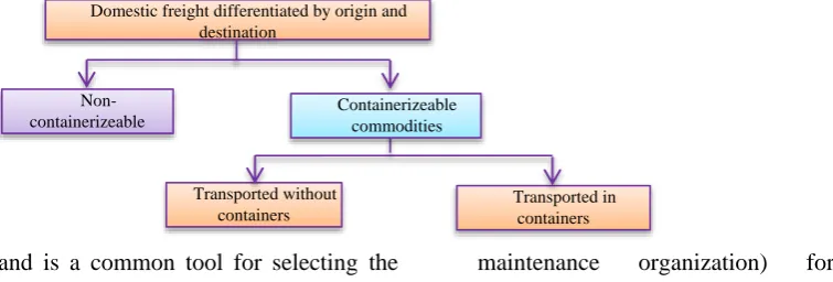
4. Modeling
Figure 2 shows the schematic framework of the model representing the tendency to use containers as the means of road-based transport. This model, hereafter called containerized transport model, is based on data pertaining to domestic bills of lading issued (by road
maintenance organization) for highly
containerizeable commodities.
Figure 2. The schematic framework of containerized transport model
Domestic freight differentiated by origin and destination
Transported without containers
Transported in containers
Non-containerizeable commodities
Modeling the Container Selection for Freight Transportation: Case Study of Iran
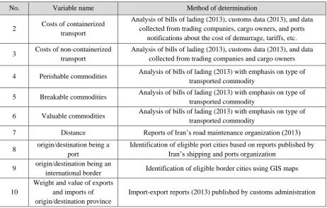
Table 5. Variables defined to build the decision tree
No. Variable name Method of determination
2 Costs of containerized transport
Analysis of bills of lading (2013), customs data (2013), and data collected from trading companies, cargo owners, and ports
notifications about the cost of demurrage, tariffs, etc.
3 Costs of non-containerized transport
Analysis of bills of lading (2013), customs data (2013), and data collected from trading companies and cargo owners
4 Perishable commodities Analysis of bills of lading (2013) with emphasis on type of transported commodity
5 Breakable commodities Analysis of bills of lading (2013) with emphasis on type of transported commodity
6 Valuable commodities Analysis of bills of lading (2013) with emphasis on type of transported commodity
7 Distance Reports of Iran’s road maintenance organization (2013)
8 origin/destination being a port
Identification of eligible port cities based on reports published by Iran’s shipping and ports organization
9 origin/destination being an
international border Identification of eligible border cities using GIS maps
10
Weight and value of exports and imports of origin/destination province
Import-export reports (2013) published by customs administration
The work started by collecting the data
pertaining to containerizeable commodities
from the bills of lading to define the variables affecting the view of cargo owners, transport companies and experts about the selection of containers as the method of road-based freight transport. According to general opinion of these groups, factors such as type of cargo, total cost of containerized and traditional transit, nature of cargo (export, import or domestic) etc. are the most important criteria affecting the selection of containers as the means of transport. On this basis, variables of Table 5 were defined to describe these factors.
Output variable was considered to be a discrete variable with two values: one (containerizablity of commodity) and zero (non-containerizablity of commodity). Other variables were added to the model based on data described in Table 4.
4.1 Costs of Containerized Transport
The cost of containerized transport (in ton-.kilometer) included the loading costs at the origin, the cost of transit to destination, unloading costs, the cost of loading, returning,
and unloading the empty containers, and a demurrage cost, which was calculated based on round-trip time.
4.2
Costs
of
Non-Containerized
Transport
The cost of non-containerized transport (in ton. kilometer) included the loading costs at the origin, the cost of transit to destination, unloading costs, plus a strip cost if cargo was imported from a maritime border. The cost of transit to destination was calculated based on transport tariffs listed on bills of lading.
5. Modeling Results
All decision tree models were developed through two phases, training and testing, using CandR, QUEST, CHAID and C5 algorithms. Results obtained by each algorithm are shown in Table 6. The fourth column of this table shows the impact of most important variables on the model.
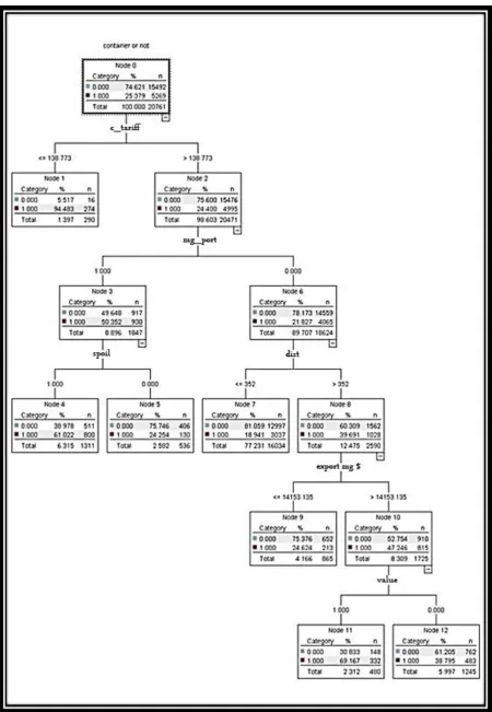
Based on these results, the pruned C5 model has provided the best combination of accuracy and simplicity and the variables identified by this method seem to be more acceptable; meanwhile, the highest accuracy has been achieved by typical C5 model. These results showed that the model developed by C5 algorithm is the best model for estimating the containerized or non-containerized transport of cargo. The model developed via pruned C5 algorithm is shown in Figure A1 of Appendix.
The rules of the developed decision tree are as follows:
The first node is related to costs ofcontainerized transport.
o If the cost of containerized transport is less
than 138.7 Tomans per ton-kilometer,
containerized and non-containerized
transport constitute, respectively, 94% and 6% of total transit. As a result this is an end-node that leads to selection of containerized transport.
o If the cost of containerized transport is
higher than 138.7 Tomans per ton-kilometer, this node is an intermediate one and leads to another node checking that whether destination is a port.
At the second node, if destination is a port
city, this node is an intermediate one and leads to another node checking that whether commodity is perishable.
At the third node, if commodity is
perishable, containerized and
non-containerized transport constitute,
respectively, 61% and 39% of total transit (perishable products are more likely to be transported by containers) so this end-node leads to selection of containerized transport.
When commodity is not perishable,
containerized and non-containerized transport constitute, respectively, 24% and 76% of total transit; so this is also an end-node but leads to selection of non-containerized transport
If destination is not a port city, this node
leads to fourth node, which checks the status of distance.
When distance is less than 352
kilometers, only 19% of freight are transported by containers and 81% are transported by traditional methods (the use of containers for long distances is more common). This is an end-node that leads to selection of non-containerized transport
When distance is more than 352
kilometers, this node is an intermediate node, which leads to another node that checks the value of exports of destination.
o If value of exports of destination is less
than 14000 dollars, containerized and non-containerized transport constitute, respectively, 24% and 76% of total transit. This is an end-node that leads to selection of non-containerized transport
o When value of exports of destination is
more than 14000 dollars, this node is an intermediate one and leads to another node checking that whether commodity is valuable.
When transported commodity is
valuable, containerized and
non-containerized transport constitute,
respectively, 70% and 30% of total transit, so the node leads to selection of containerized transport
When transported commodity is notvaluable, the fraction of freights transported by container decreases to 38% against 62% transported by traditional methods, so the node leads to
Modeling the Container Selection for Freight Transportation: Case Study of Iran
Table 6. An instance of data prepared for decision tree based modeling
No. decision tree algorithm
Depth of
the tree The effective variables (the extent of effect)
Correct prediction (%) Test phase Test phase
1 CandR 4 Perishable commodities (49%), distance (26%), destination (15%), type
of commodity (8%) origin (2%) 78.11 70.24
2 CHAID 5 Perishable commodities (35%), breakable commodities (32%), distance
(20%), the value of exports of origin (5%) 78.16 71.01
3 QUEST 5 the weight of exports of origin (37%), the value of exports of origin
(36%), type of commodity (13%) perishable commodities (10%) 76.61 69.18
4 C5 8
Perishable commodities (30%), container tariffs (23%), distance (18%), breakable commodities (11%), destination (7%), destination being a port
(7%), valuable commodities (2%)
79.87 71.89
5 Pruned C5 5 Container tariffs (29%), destination being a port (26%), distance (21%),
perishable commodities (21%) and value of export of destination (4%) 78.18 71.45
6. Conclusion
This study used, CHAID, QUEST, C5 and C$R algorithms to develop a decision tree to determine the tendency toward containerized
mode of transport in road-based
transportations. The results showed that the decision tree built via full C5 algorithm provides the best accuracy; the disadvantage of this algorithm however was its great size, which was eliminated to some extent by pruning. The resulting pruned C5 model has a slightly lower accuracy but provides the best combination of accuracy and simplicity. The most important variables affecting the model were the cost of containerized transport (C_Tariff), the status of destination (whether it is a port) (Mg_port), distance (Dist), perishability of transported commodity (Spoil), and value of exports made by destination (Export mg $). Model was able to predict 78.14% of the data correctly. High-value and perishable commodities had the greatest potential for containerized transport. The most important policy factors that could affect the decision of cargo owners to use containerized transport are tariffs on this mode of transit and the status of destination (whether it is a port). Policies that could encourage cargo owners to use intermodal transport include setting a lower tariff on container handling, reducing the cost of loading and unloading, increasing the port facilities supporting the containerized transport, adjusting customs, and
development of dry ports
.
7. References
- Abdelwahab, W. and Sayed, T. (1999)
“Freight mode choice models using artificial neural networks”, Civil Engineering Systems, Vol. 16, No. 4, pp. 267-286.
- Degerland, J. (2011) “Containerisation
International Year Book”, source: Baird
Maritime, April, 2011. Website:
www.informacargo.com/ciyb
- Esmaeili, M. (2014)“ Concepts and methods
of data mining”, Iran: Green Publishing E-book", First Edition.
- Fowkes, A. S., Nash, C. A. and Twedle, G.
(1991) “Investigating the market for
intermodal freight technologies”,
Transportation Research Part A, Vol. 25, No. 4, pp. 161-172.
- Kass, G.V. (1980) “An exploratory
technique for investigating large quantities of categorical data”. Applied statistics, Vol. 29, No. 2, p. 119.
- Kotsians, S. B. (2007) “Supervised machine
learning: A review of classification techniques”, Vol. 31, No. 3, pp. 249-268.
- Mohri, S. S. and Haghshenas, H. (2015)
M.Sc.Thesis, Isfahan University of Technology.
- Ortuzar, J. D. and Palma, A. (1988) “Stated
preference in refrigerated and frozen cargo exports”, Simplified Transport Demand Modelling, Perspective 2, PTRC, London.
- Quinlan, J. R. (2014) “C4. 5: programs for
machine learning”, USA: Elsevier.
- Rashidi, T. H. and Mohammadian, A.
(2011) “Household travel attributes
transferability analysis: application of a
hierarchical rule based approach”,
Transportation, Vol. 38, NO.4, pp. 697-714.
- Ravibabu, M. (2013) “A nested logit model
of mode choice for inland movement of export shipments: A case study of containerised export cargo from India”, Research in Transportation Economics, Vol. 38, No. 1, pp. 91-100.
- Sayed, T. and Razavi, A. (2000)
“Comparison of neural and conventional approaches to mode choice analysis”, Journal of Computing in Civil Engineering, Vol. 14, No. 1, pp. 23-30.
- Shinghal, N. and Fowkes, T. (2002) “Freight
mode choice and adaptive stated
preferences”, Transportation Research Part E, Vol. 38, No. 5, pp. 367-378.
- Tortum, A., Yayla, N. and Gökdağ, M.
(2009) “The modeling of mode choices of intercity freight transportation with the artificial neural networks and adaptive neuro-fuzzy inference system”, Expert Systems with Applications, Vol. 36, No. 3, pp. 6199-6217.
- UNCTAD (2012) “Review of maritime
transport”, source: United Nations
Conference on Trade and Development, 04
Dec 2012, 196 pages, Website:
www.unctad.org
- Vieira, L. F. M. (1992) “The value of service
in freight transportation”, PhD Thesis. Massachusetts Institute of Technology, Cambridge, MA. USA: MIT Libraries.
- Winston, C. M. (1981) “A multinomial
model for prediction of the demand for domestic ocean container service”, Journal of Transport Economics and Policy, Vol. 15, No. 3, pp. 243-252.
- Xie, C., Lu, J. and Parkany, E. (2003) “Work
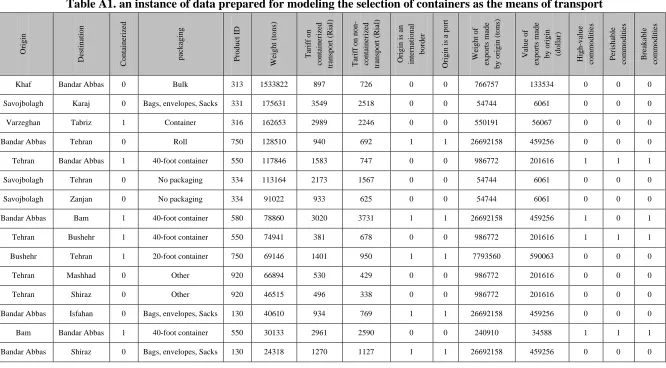
Table A1. an instance of data prepared for modeling the selection of containers as the means of transport
Origin Destin atio n Co n tain erize d p ackag in g Prod u ct I D W eig h t ( to n s) Tar if f o n co n tain erize d trans p o rt (Rial ) Tar if f o n no n -co n tain erize d trans p o rt (Rial ) Origin is an in ternatio n al b o rder Origin is a p o rt W eig h t of ex p o rts m ad e b y orig in ( to n s) Valu e of ex p o rts m ad e b y orig in (do llar) Hig h -v alu e co m m o d ities Perish ab le co m m o d ities Breakab le co m m o d itiesKhaf Bandar Abbas 0 Bulk 313 1533822 897 726 0 0 766757 133534 0 0 0
Savojbolagh Karaj 0 Bags, envelopes, Sacks 331 175631 3549 2518 0 0 54744 6061 0 0 0
Varzeghan Tabriz 1 Container 316 162653 2989 2246 0 0 550191 56067 0 0 0
Bandar Abbas Tehran 0 Roll 750 128510 940 692 1 1 26692158 459256 0 0 0
Tehran Bandar Abbas 1 40-foot container 550 117846 1583 747 0 0 986772 201616 1 1 1
Savojbolagh Tehran 0 No packaging 334 113164 2173 1567 0 0 54744 6061 0 0 0
Savojbolagh Zanjan 0 No packaging 334 91022 933 625 0 0 54744 6061 0 0 0
Bandar Abbas Bam 1 40-foot container 580 78860 3020 3731 1 1 26692158 459256 1 0 1
Tehran Bushehr 1 40-foot container 550 74941 381 678 0 0 986772 201616 1 1 1
Bushehr Tehran 1 20-foot container 750 69146 1401 950 1 1 7793560 590063 0 0 0
Tehran Mashhad 0 Other 920 66894 530 429 0 0 986772 201616 0 0 0
Tehran Shiraz 0 Other 920 46515 496 338 0 0 986772 201616 0 0 0
Bandar Abbas Isfahan 0 Bags, envelopes, Sacks 130 40610 934 769 1 1 26692158 459256 0 0 0
Bam Bandar Abbas 1 40-foot container 550 30133 2961 2590 0 0 240910 34588 1 1 1
Modeling the Container Selection for Freight Transportation: Case Study of Iran