University of Mazandaran, Iran http://cjms.journals.umz.ac.ir ISSN: 2676-7260 CJMS.9(1)(2020), 124-136
A Novel Successive Approximation Method for Solving a Class of Optimal Control Problems
M. Shirazian 1 and S. Effati2
1 Department of Mathematics, University of Neyshabur, Neyshabur, Iran.
2 Department of Applied Mathematics, Ferdowsi University of Mashhad, Mashhad, Iran.
Abstract.This paper presents a successive approximation method (SAM) for solving a large class of optimal control problems. The proposed analytical-approximate method successively solves the Two-Point Boundary Value Problem (TPBVP), obtained from the Pon-tryagin’s Maximum Principle (PMP). The convergence of this method is proved and a control design algorithm with low computational complexity is presented. Through the finite number of algorithm iterations, a suboptimal control law is obtained for the optimal con-trol problem. An illustrative example is given to show the efficiency of the proposed method.
Keywords:Optimal control problem, Successive approximation method, Pontryagin’s maximum principle, Suboptimal control.
2000 Mathematics subject classification: 49K15; Secondary 49M05.
1. Introduction
In the control theory, a major importance is conferred to optimal con-trol problems. This interest is justified by a great number of practical applications in physics, economy, aerospace, chemical engineering, ro-botics, etc. [5, 15, 14, 20, 7]. For the general optimal control problem
1Corresponding author: [email protected]
Received: 15 October 2019 Revised: 9 November 2019 Accepted: 13 November 2019
(OCP), however, an analytical solution does not exist. This has inspired researchers to propose approaches which obtain an approximate solution for it.
It is well-known that the OCP leads to a TPBVP obtained from the PMP. Many recent approaches have been devoted to solving this prob-lem. One of these approaches is the Successive Approximation Approach (SAA) which designs a suboptimal controller for a class of nonlinear sys-tems with a quadratic performance index. In this approach, a sequence of nonhomogeneous linear time-varying TPBVP’s is solved to produce a finite-step iteration of the nonlinear compensation sequence obtaining the suboptimal control law [19]. However, SAA needs to solve a linear time-varying TPBVP which cannot be solved easily and thus, reduces the efficiency of this method.
In [11], a novel method that implements Modal series to solve a class of nonlinear OCP’s with quadratic performance index has been proposed. This method which requires solving a sequence of linear time-invariant TPBVP’s has less efficiency for large-scale problems.
Recently, a growing interest has been appeared toward the application of approximate analytical techniques in solving the TPBVP obtained from the PMP. In [22], the authors used He’s variational iteration method (VIM) for linear quadratic OCP’s. They transfer the linear TPBVP obtained from PMP to an initial value problem and then implement the VIM to get a feedback controller. Although their proposed method is important for its analytical approximation solutions, it is not applicable for nonlinear OCP’s.
In [4], the authors give an analytical approximate solution for linear and non-linear quadratic OCP’s using the homotopy perturbation method (HPM). Applying the HPM, the associated TPBVP is solved recursively and gets a suboptimal control law. Also, in [18], a basic and a modified VIM are successfully applied to the TPBVP, obtained from nonlinear quadratic OCP’s. The authors combined the basic ideas of the shooting method to VIM and get the solutions consecutively. Though both of these two methods give accurate results, they suffer from a root-finding subroutine and then solving a system of algebraic equations which de-creases the efficiency of the proposed methods.
methods for solving more general optimal control problems are also avail-able ate.g. [8], [10].
In this paper, a novel SAM is proposed. We first derive the TPBVP from the PMP and then apply a novel SAM to solve it. This method could be applied to a large class of linear and nonlinear OCP’s. The convergence of the proposed method is proved and a suboptimal con-trol design algorithm with low computational complexity is presented. The simplicity and the efficiency of the proposed SAM is demonstrated through an illustrative example.
This paper is organized as follows. Section 2 describes the OCP and its associated extreme conditions. The novel SAM for solving the TPBVP is proposed in Section 3. The convergence of the proposed method is proved in section 4. In section 5, an efficient control design algorithm is presented. And finally, an illustrative example is given in section 6 to demonstrates the effectiveness of the new SAM.
2. Statement of the OCP and optimality conditions
Consider the following affine in control dynamical system
˙
x(t) =f(t, x(t)) +g(t, x(t))u(t), t∈[t0, tf]
x(t0) =x0.
(2.1)
where x(t) ∈ Rn is denoting the state variable, u(t) ∈ Rm the control variable and x0 the given initial state at t0. Moreover, f(t, x(t))∈ Rn and g(t, x(t)) ∈ Rn×m are two continuously differentiable functions in all arguments. Our aim is to minimize the objective functional
J[x, u] = 1 2
∫ tf
t0
(Q(x(t)) +uT(t)Ru(t))dt (2.2)
subject to the dynamical system (2.1), for Q(x(t)) a positive semi-definite real function and R ∈ Rm×m a positive definite matrix. Since the performance index (2.2) is convex, the following extreme necessary conditions are also sufficient for optimality:
˙
x=f(t, x) +g(t, x)u∗ ˙
λ=−Hx(x, u∗, λ)
u∗ = arg minuH(x, u, λ)
x(t0) =x0, λ(tf) = 0.
(2.3)
([4, 18]):
˙
x=f(t, x) +g(t, x)[−R−1gT(t, x)λ] ˙
λ=−
(
1
2∇Q(x) + ( ∂f(t,x)
∂x )
Tλ+∑n
i=1λi[−R−1gT(t, x)λ]T ∂gi∂x(t,x)
)
x(t0) =x0, λ(tf) = 0.
(2.4) where λ(t) ∈ Rn is the co-state vector with the ith component λi(t),
i = 1, ..., n and g(t, x) = [g1(t, x), ..., gn(t, x)]T with gi(t, x) ∈ Rm, i =
1, ..., n. Also the optimal control law is obtained by
u∗ =−R−1gT(t, x)λ. (2.5)
For convenience, let us define the right hand sides of (2.4) as,
Ψ1(t, x, λ) :=f(t, x) +g(t, x)[−R−1gT(t, x)λ], Ψ2(t, x, λ) :=−
(
1
2∇Q(x) + ( ∂f(t,x)
∂x )
Tλ+∑n
i=1λi[−R−1gT(t, x)λ]T ∂gi∂x(t,x)
)
. (2.6) Thus the TPBVP in (2.4) changes to the operator form ([9, 21]) as follows:
˙
X(t)−Ψ(t, X(t)) =L[X(t)] +N[X(t)] = 0, x(t0) =x0, λ(tf) = 0,
(2.7)
where
X(t) =
[
x(t) λ(t)
]
, Ψ(t, X(t)) =
[
Ψ1(t, X(t)) Ψ2(t, X(t))
]
,
and the linear and nonlinear operatorsL and N are defined as:
L[X(t)] = ˙X(t) +p(t)X(t),
N[X(t)] =−p(t)X(t)−Ψ(t, X(t)) =
[
N1[X(t)] N2[X(t)]
]
, (2.8)
wherep(t)is a real (2n) by(2n)matrix as follows:
p(t) =
[
p1(t) O O p2(t)
]
, p1(t), p2(t)∈Rn×n.
3. A New SAM for Solving the TPBVP
In this section, we propose a new SAM to solve the TPBVP in (2.7), analytically. Construct a sequence of solutions for solving (2.7), as fol-lows:
L[Xk+1(t)] =−N[Xk(t)], (3.1) withxk+1(t0) =x0,λk+1(tf) = 0and k≥0. This linear ODE could be solved forxk+1(t)analytically (See e.g. [3, 17]).
In view of (2.8), solving (3.1) leads to:
Xk+1(t) =−
∫ t
t0
Φ(t, s)N[Xk(s)]ds+ Φ(t, t0)C, (3.2)
where Φ(t, s) = e−∫stp(τ)dτ is the transfer matrix and C ∈ R2n is con-stant. (3.2) can be equivalently written as:
xk+1(t) =−
∫t
t0Φ1(t, s)N1[Xk(s)]ds+ Φ1(t, t0)C1, λk+1(t) =−
∫t
t0Φ2(t, s)N2[Xk(s)]ds+ Φ2(t, t0)C2.
(3.3)
where the transfer matrix is decomposed as follows:
Φ(t, s) =
[
Φ1(t, s) O O Φ2(t, s)
]
,∀s∈[t0, t]andt∈[t0, tf],
andΦi(t, s) =e−
∫t
spi(τ)dτ,i= 1,2. AlsoΦ
i(t, s)·Φi(s, w) = Φi(t, w), for allt, s, w∈[t0, tf]andi= 1,2. Imposing the initial and final conditions,
xk+1(t0) =x0 and λk+1(tf) = 0, for allk≥0,C1 and C2 can be readily calculated as:
C1 = x0,
C2 = Φ−21(tf, t0)
∫tf
t0 Φ2(tf, s)N2[Xk(s)]ds =∫tf
t0 Φ2(t0, tf)Φ2(tf, s)N2[Xk(s)]ds =∫tf
t0 Φ2(t0, s)N2[Xk(s)]ds.
Therefore, the SAM formula becomes,
xk+1(t) = −
∫ t
t0
Φ1(t, s)N1[Xk(s)] + Φ1(t, t0)x0, (3.4)
λk+1(t) =
∫ tf
t
Φ2(t, s)N2[Xk(s)]ds. (3.5)
correction, which omits the time consuming calculations from SAM can be applied:
xk+1(t) =−
∫t
t0Tk(t, s)ds+ Φ1(t, t0)x
0, λk+1(t) =
∫tf
t Tek(t, s)ds.
(3.6)
whereTk(t, s)andTek(t, s)are thekthorder of Taylor interpolating poly-nomial ats=t0 of the integrands of (3.4) and (3.5), respectively.
4. Convergence Analysis
Now, we state and prove the convergence of the foregoing SAM se-quence.
Definition 4.1. ([2]) LetV be a Banach space. For an operatorT :K⊆ V →V, we say it is contractive with contractivity constantα∈[0,1), if
∥T(v)−T(w)∥V ≤α∥v−w∥V, ∀v, w∈K.
Theorem 4.2. Assume that{xk(t)}and{λk(t)}are two SAM sequences produced by (3.4)-(3.5). Furthermore, assumeN[v(t)] is continuous for anyv(t)∈R2n, t∈[t0, tf], and
|N[v(t)]−N[w(t)]| ≤M1|v(t)−w(t)|, ∀v, w ∈C[t0, tf], for some constantM1. Then {xk(t)} and {λk(t)} converge to the exact solutions of (2.7), for any initial continuous functions x0(t) and λ0(t), if the contractivity constant M1M2(tf −t0)∈[0,1), where
M2 = sup
{
e−∫stp(τ)dτ, s∈[t0, t], t∈[t0, tf]
}
.
Proof. It is clear that the SAM sequences (3.4)-(3.5) are equivalent to (3.1) or (3.2). In the light of (3.2), define the operator T as:
T[v(t)] :=−
∫ t
t0
e−∫stp(τ)dτN[v(s)]ds+e−
∫t
t0p(τ)dτC, C ∈R2n. (4.1)
Then for any continuous functionsv(t) andw(t), we have:
|T[v(t)]−T[w(t)]| =
∫ t
t0
e−∫stp(τ)dτ(N[v(s)]− N[w(s)])ds
≤ M2
∫tt
0
(N[v(s)]− N[w(s)])ds
≤ M1M2
∫ t
t0
|v(s)−w(s)|ds
Thus by Banach fixed-point theorem (page 133 of [2]), {xk(t)} and {λk(t)} converge to some x(t)ˆ and ˆλ(t). By taking limits from both sides of (3.1), we have:
lim
k→∞L[Xk+1] =−klim→∞N[Xk], which the continuity of N, gives
L[ lim
k→∞Xk+1] =−N[ limk→∞Xk],
orL[ ˆX] =−N[ ˆX]. Moreover, by (3.4)-(3.5), one can easily check that for all k ≥ 0, xk+1(t0) = x0 and λk+1(tf) = 0. Hence, x(tˆ 0) = x0 and ˆ
λ(tf) = 0. That is, x(t)ˆ and λ(t)ˆ are the exact solutions of (2.7) which
completes the proof. □
Remark 4.3. The choice of p(t)should be performed such that the con-ditionM1M2(tf −t0) ∈[0,1) in Theorem 4.1 holds. Some easy choices could be zero matrix, the linear parts at each equation of (2.4) or some linear term that we add to the both sides of equations in (2.4).
Theorem 4.4. Under the assumptions of Theorem 4.2, the sequences {uk(t)} and {Jk} defined by
uk(t) = −R−1gT(t, xk(t))λk(t), (4.2)
Jk =
1 2
∫ tf
t0
(Q(xk(t)) +uTk(t)Ruk(t))dt, (4.3)
converge to the optimal control law and optimal objective value, respec-tively.
Proof. Theorem 4.2 states that {xk(t)}and {λk(t)}converge to the op-timal state and costate vectors, say x(t)ˆ and λ(t)ˆ , respectively. Taking limits from (4.2), the continuity assumption ofg(t, x)gives
ˆ
u(t) := lim
k→∞uk(t) =−R
−1gT(t, lim
k→∞xk(t)) limk→∞λk(t)
= −R−1gT(t,x(t))ˆˆ λ(t),
which is the optimal control law, since x(t)ˆ and λ(t)ˆ are the optimal state and costate vectors. Also by the continuity assumption ofQ(x(t)), taking limits from (4.3) yields:
ˆ
J := lim
k→∞Jk=
1 2klim→∞
∫ tf
t0
(Q(xk(t)) +uTk(t)Ruk(t))dt
= 1 2
∫ tf
t0
(Q( lim
k→∞xk(t)) + limk→∞u T
k(t)R lim
k→∞uk(t))dt
= 1 2
∫ tf
t0
ThereforeJˆis the optimal objective value. □
5. Suboptimal control design algorithm
The solution guidelines for TPBVP (2.7) has been discussed in previ-ous section. In this section, we give a more reliable way for finding the desired optimal control and the optimal state and then we present an algorithm for this end.
From Theorem 4.4, we conclude that for large number of iterations, N, suboptimal control law is derived by
u∗(t)∼=uN(t) =−R−1gT(t, x)λN(t), (5.1)
and the approximate suboptimal state is x∗(t) ∼=xN(t). Applying this pair of suboptimal control and state to the objective functional (2.2), results in the suboptimal objective value of the problem, i.e.
J∗∼=JN =
1 2
∫ tf
t0
(Q(xN(t)) +uTN(t)RuN(t))dt. (5.2)
For the accuracy analysis, we consider the following criterion. The sub-optimal control (5.1) has the desirable accuracy, if for givenϵ > 0, the following condition holds,
JN −JN−1
JN
< ϵ. (5.3)
If the tolerance limit ϵ is sufficiently small, according to Theorem 4.4, the suboptimal value is very close to the optimal value J∗. Now, we present an algorithm of the proposed method with low computational complexity, in order to maintain the accuracy of solutions.
Algorithm:
Step 1. Let N = 1, x0(t) = x0, λ0(t) = 0 and ϵ > 0 be any given sufficiently small tolerance.
Step 2. Update state and costate functions implementing the SAM (3.4)-(3.5) or (3.6), to findxN(t) and λN(t).
Step 3. Determine the suboptimal control uN(t) and the suboptimal objective valueJN by (5.1)-(5.2).
Step 4. If criterion (5.3) holds, go to Step 5, otherwise letN =N+ 1 and go to Step 2.
6. Illustrative example
The following example is given to illustrate the simplicity and effi-ciency of the proposed method. The codes are developed using com-putation softwares MAPLE 15 and MATLAB, and the calculations are implemented on a machine with Intel Core 2 Due Processor 2.53 Ghz and 4 GB RAM.
Example 6.1. Consider the nonlinear system described by
˙
x1 =x2+x1x2 ˙
x2 =−x1+x2+x22+u x1(0) =−0.8, x2(0) = 0
(6.1)
and the cost functional
J = 1 2
∫ 1
2
0
(x21+x22+u2)dt. (6.2)
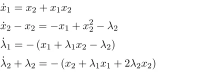
The extreme conditions are ˙
x1=x2+x1x2 ˙
x2=−x1+x2+x22−λ2 ˙
λ1=−(x1+λ1x2−λ2) ˙
λ2=−(x2+λ1(1 +x1) +λ2(1 + 2x2))
x1(0) =−0.8, x2(0) = 0, λ1(12) = 0, λ2(12) = 0,
and the optimal control isu=−λ2. In view of (2.8), the linear and the nonlinear operators of the above TPBVP can be defined in several ways as follows:
L[X] = ˙X(t) +p(t)X(t), whereX= [x1, x2, λ1, λ2]T and
(a)
p(t) = O4×4, N[X] =
−x2−x1x2 x1−x2−x22+λ2
x1+λ1x2−λ2
x2+λ1(1 +x1) +λ2(1 + 2x2)
, α= 0.4016
(b) p(t) =
0 −1 0 0 1 −1 0 0 0 0 0 −1
0 0 1 1
, N[X] =
−x1x2 −x22+λ2 x1+λ1x2 x2+λ1x1+ 2λ2x2
, α= 0.6554
Table 1. Simulation results of SAM in case (a) and (b), based on the relative errors of objective value, Example 1.
N (Itr.) Case (a) Case (b) 5 4.82861×10⁻³ 9.30044×10⁻³ 10 9.64918×10⁻⁵ 1.36117×10⁻⁴ 15 1.58638×10⁻⁶ 1.24144×10⁻⁶ 20 4.89518×10⁻⁸ 1.08149×10⁻⁸ 25 2.23602×10⁻¹⁰ 7.22779×10⁻¹¹
(b), p(t) is linear terms of each equation in extreme conditions. i.e. the extreme conditions are written as:
˙
x1 =x2+x1x2 (6.3)
˙
x2−x2=−x1+x22−λ2 (6.4) ˙
λ1 =−(x1+λ1x2−λ2) (6.5) ˙
λ2+λ2 =−(x2+λ1x1+ 2λ2x2) (6.6) The left hand sides of the above equation are the linear parts and the right hand sides are nonlinear terms. Of course, other choices are avail-able as discussed in Remark 4.3. It is important to note that the con-vergence of SAM is guaranteed wheneverα ∈[0,1), which is true in our case (a) and (b).
Implementing the algorithm described in Section 5, one can obtain the suboptimal solution for given ϵ = 5×10⁻⁶, after N = 15 iterations. Table 1 shows the relative error of optimal objective values for several iterations. It is seen that SAM (a) and (b) reach the tolerance limit after 15 iterations. For N = 15, the suboptimal control and objective value can be found using SAM (a) as:
u∗(t)∼=u15(t) = 8.2005×10⁻⁷ t16+ 0.23575×10⁻⁵ t15−0.18623×10⁻⁴ t14
−0.12099×10⁻⁴ t13−0.10112×10⁻³ t12−0.16282×10⁻³ t11+ 0.59612×10⁻³ t10
+0.21462×10⁻³ t9+ 0.21739×10⁻² t8+ 0.27712×10⁻²t7−0.022487t6
−0.78086×10⁻² t5−0.036403t4−0.035923t3+ 0.49182t2+ 0.049226t−0.14024,
J∗∼=J15= 0.175683.
To illustrate the efficiency of the proposed method, we compare the results of SAM (a), with two recent methods, VIM [18] and HPM [4]. The number of iterations and the CPU time of these methods are sum-marized in Table 2, for different tolerance limits (5.3).
0 0.1 0.2 0.3 0.4 0.5 −0.8
−0.795 −0.79 −0.785 −0.78
t
State function x
1
(t)
Proposed SAM Modified VIM Collocation method
0 0.1 0.2 0.3 0.4 0.5 0
0.1 0.2 0.3 0.4 0.5
t
State function x
2
(t)
Proposed SAM Modified VIM Collocation method
Figure 1. The suboptimal states of Example 1.
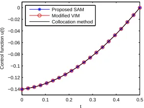
0 0.1 0.2 0.3 0.4 0.5 −0.14
−0.12 −0.1 −0.08 −0.06 −0.04 −0.02 0
t
Control function u(t)
Proposed SAM Modified VIM Collocation method
Figure 2. The suboptimal control of Example 1.
Table 2. Comparison of the proposed SAM, Modified VIM [18] and HPM [4], Example 1.
Tolerance Proposed SAM Modified VIM [18] HPM [4] limit (ϵ) N CPU Time∗ N CPU Time N CPU Time
5×10⁻⁶ 15 0.266 10 0.546 11 8.752
5×10⁻⁹ 22 0.406 17 2.761 -
-5×10⁻¹² 29 0.811 23 15.71 -
-* CPU time (sec.)
not. In fact, HPM could not reach the tolerance limit less than5×10−9, because of the complicated calculations and the CPU time of the modi-fied VIM grows rapidly for a large number of iterations.
Table 3. Comparison of objective values of the pro-posed SAM (a)-(b), Modified VIM [18] and HPM [4] for m= 10iterations, Example 1.
Method Jm
Proposed SAM (a) 0.1756936822 Proposed SAM (b) 0.1756786212 Modified VIM 0.1756827686
HPM 0.1756827686
approximately J∗ = 0.1757. Figures 1 and 2 show the suboptimal solu-tions afterN = 15algorithm iterations, compared to the Modified VIM and collocation method [13].
7. Conclusions
In this paper, a novel analytical approximate method called SAM has been proposed for solving a broad class of optimal control problems. This method can solve the TPBVP obtained from PMP recursively. The proposed SAM does not need any complex computations in comparison with other recent methods. The convergence of the proposed SAM is proved and an illustrative example demonstrated the effectiveness and good results in low CPU time.
References
1. M. Alipour, M. A. Vali, and A. H. Borzabadi, A hybrid parametrization approach for a class of nonlinear optimal control problems, Numerical Al-gebra, Control & Optimization, 9(4)(2019) 493-506.
2. K. Atkinson, and W. Han, Theoretical numerical analysis: a functional analysis framework,Springer, 2009.
3. C. K. Chui, and G. Chen, Linear systems and optimal control. Vol. 18. Springer Science & Business Media, 2012.
4. S. Effati and H. Saberi Nik, Solving a class of linear and non-linear opti-mal control problems by homotopy perturbation method,IMA Journal of Mathematical Control and Information,28(2011) 539-553.
5. W.L. Garrard and J.M. Jordan , Design of nonlinear automatic flight con-trol systems,Automatica,13(5) (1997) 497-505.
6. S. Ganjefar and S. Rezaei, Modified homotopy perturbation method for optimal control problems using Pade approximant, Applied Mathematical Modelling, 40(2016) 7062–7081.
7. X. Gao, K. L. Teo and G. R. Duan, An optimal control approach to space-craft rendezvous on elliptical orbit,Optim. Control Appl. Meth.,36(2015) 158-178.
9. A. Ghorbani, and M. Tavakoli, An Adaptive Spectral Parametric Method for Solving Nonlinear Initial Value Problems,Bulletin of the Iranian Math-ematical Society,45(3) (2019) 737-754.
10. A. Jajarmi, M. Hajipour, E. Mohammadzadeh and Dumitru Baleanu, A new approach for the nonlinear fractional optimal control problems with external persistent disturbances, Journal of the Franklin Institute, 355 (2018) 3938–3967
11. A. Jajarmi, N. Pariz, A. V. Kamyad and S. Effati, A novel modal se-ries representation approach to solve a class of nonlinear optimal control problems,International Journal of Innovative Computing, Information and Control, 7(3)(2011) 1413-1425.
12. W. Jia, X. He and L. Guo, The optimal homotopy analysis method for solving linear optimal control problems, Applied Mathematical Modelling, 45 (2017) 865–880.
13. J. Kierzenka and L. F. Shampine, A BVP Solver based on residual con-trol and the MATLAB PSE,ACM Transactions on Mathematical Software, 27(3) (2001) 299-316.
14. T. Konishi, M. Notsu and J. Imai , Optimal water cooling control for plate rolling,Int. J. Innov. Comput. Inform. Control,4(12) (2008) 3169-3181. 15. V. Manousiouthakis and D.J. Chmielewski, On constrained infinite-time
nonlinear optimal control,Chem. Eng. Sci.,57(1) (2002) 105-114. 16. H. Mirinejad and T. Inanc, An RBF collocation method for solving optimal
control problems, Robotics and Autonomous Systems,87 (2017) 219–225. 17. H. M. Moya-Cessa, and F. Soto-Eguibar, Differential equations: an
opera-tional approach. Rinton Press, Incorporated, 2011.
18. M. Shirazian and S. Effati, Solving a Class of Nonlinear Optimal Control Problems via He’s Variational Iteration Method,International Journal of Control, Automation, and Systems,10(2)(2012) 249-256.
19. G. -Y. Tang, Suboptimal control for nonlinear systems: a successive ap-proximation approach,Systems & Control Letters,54(2005) 429-434. 20. L. Tang, L.D. Zhao and J. Guo, Research on pricing policies for seasonal
goods based on optimal control theory,ICIC Expr. Lett.,3(4B) (2009)1333-1338.
21. R. A. Van Gorder, Optimal homotopy analysis and control of error for im-plicitly defined fully nonlinear differential equations,Numerical Algorithms 81(1) (2019) 181-196.
![Table 3.Comparison of objective values of the pro-posed SAM (a)-(b), Modified VIM [18] and HPM [4] form = 10 iterations, Example 1.](https://thumb-us.123doks.com/thumbv2/123dok_us/10118959.1999281/12.612.182.353.111.184/table-comparison-objective-values-posed-modified-iterations-example.webp)
