A Fast Calculation Method for Analyzing the Effect of Wind
Generation on ATC
M. A. Armin* and H. Rajabi Mashhadi**(C.A.)
Abstract: Wind energy penetration in power system has been increased very fast and large amount of capitals invested for wind farms all around the world. Meanwhile, in power systems with Wind Turbine Generators (WTGs), the value of AVAILABLE TRANSFER CAPABILITY (ATC) is influenced by the probabilistic nature of the wind power. The Mont Carlo Simulation (MCS) is the most common method to model the uncertainty of WTG. However, the MCS method suffers from low convergence rate. To overcome this shortcoming, the proposed technique in this paper uses a new formulation for solving ATC problem analytically. This lowers the computational burden of the ATC computation and hence results in increased convergence rate of the MCS. Using the proposed method, ATC is calculated based on one step computations while numerous steps is required for ATC calculation in iterative computational methods. Using this fast technique to evaluate the ATC, wind generation and load correlation is required to get into modeling. A numerical method is presented to consider load and wind correlation. The proposed method is tested on the modified IEEE 118 bus to analyze the impacts of the WTGs on the ATC. The obtained results show that wind generation capacity and its correlation with system load has significant impacts on the network transfer capability. It is shown descriptively that a complex and nonlinear relation exist among ATC distribution function, WTG capacity and network topography.
Keywords: Copula, Correlation, Effective Load Carrying Capability, Reliability Indices, Wind Power Generation.
1 Introduction1
1.1 Motivations and Aims
Available Transfer Capability (ATC) is an important parameter in analyzing market behavior and system reliability [1] that indicates the capability of transferring power between generation nodes and the loads. In conventional power system, generated power has been adjusted and transferred to supply the load. In contrast to conventional generation, due to the stochastic and uncontrollable nature of the wind generation, wind power has to be transferred to where it is needed or to be curtailed. According to this compulsive transferring, ATC of the system will change. However, determining
Iranian Journal of Electrical & Electronic Engineering, 2015. Paper first received 26 Apr. 2015 and in revised form 01 Aug. 2015. * The Author is with the Department of Electrical Engineering, Ferdowsi University of Mashhad, Mashhad, Iran.
** The Author is with the Department of Electrical Engineering and the Center of Excellence on Soft Computing and Intelligent Information Processing, Ferdowsi University of Mashhad, Mashhad, Iran.
E-mails: [email protected] and [email protected].
effects of Wind Turbine Generators (WTGs) on ATC, including all possible wind generation level in ATC calculations, increases the computational burden. Hence, developing a dependable method for fast and accurate calculation of the ATC is of importance and deserves particular attention.
1.2 Literature Review
Transmission management and determination of the ATC have been carried out in several researches in a deregulated environment [2]. In the market structure, there are various sources of the uncertainties involved in the ATC calculation which increase the calculation time. Because of these conditions, fast calculation methods have been developed in various papers, such as [3, 4]. Sensitivity-based approaches, such as Power Transfer Distribution Factors (PDTF) [2], have been used in some studies for ATC calculations [5]. DC and AC load flow have been employed in the PDTF method for ATC calculation [1, 5]. Although, the AC load flow is accurate, but it increases the calculation time [6]. On the other hand, the DC load flow is very fast and easy to understand for all market participants [7].
For analyzing the effect of the uncertainties on the ATC, probabilistic approaches can be used instead of deterministic ones. Probabilistic approaches provide more information [8]. Monte Carlo simulation (MCS) [1, 9-12] and state selection method [13] have been adopted for determination of the ATC distribution.
The impact of wind power penetration on calculation ATC has been analyzed in recent works. In [14], a clustering technique is used to select the samples for fast calculation of ATC. Wind speed correlation has been analyzed in [14]. In [15] a partitioning method presented for power system to increase the speed of ATC calculation to considering effect of distributed generation in the distribution network. In this paper, historical data for wind generation and load are used to develop scenarios for MCS. In [16] some equations developed to speed up the calculation time of Continuation Power Flow (CPF) methods. CPF method and MSC are used in [17] to calculate risk for nondispatchable wind generations. CPF suffers from slow speed convergence [17] and in combination with MCS, the calculation time extremely increase. In [18], a DC optimal power flow is used for net transfer capacity (NTC) calculation in Germany. In this paper, renewable generation effects on NTC have been analyzed and they are proposed market mechanism to manage congestions.
1.3 Proposed Approach and Contributions Mainly, this paper studies the effect of wind speed and load correlation on the ATC distribution. Considering the uncertainties and different scenarios, calculation time is a serious challenge. To reduce the computation time, a time efficient and practical calculation method is proposed in this paper. In the first stage, The ATC Calculation problem is stated as an optimization problem where the aim is to maximize ATC subject to the load flow equations and transmission line capacity constraints. Considering DC load flow, the optimization problem is simplified into a linear optimization problem and consequently the optimal solution is obtained analytically. The basic idea is to interpret the concept of ATC as the amount of the transferred power through the network which activates the transmission constraints.
In the next stage of this paper, wind generation and load correlation effect on ATC has been analyzed. Considering Wind speed probability, probability distribution of wind generation can be determined according to wind turbine power curve. While wind power generation and system load has a specified correlation related to the characteristic of the studied system. Considering joint Cumulative Mass Function (CMF) of wind speed and system load, a numerical method has presented to generate simultaneously samples for these random variables. Finally, the MCS technique and presented fast technique are utilized to efficiently obtain probability mass function (PMF) of the ATC.
1.4 Paper Organization
This paper is organized as follows. A Fast technique is presented in section 2. In Section 3, the Monte Carlo simulation data, such as load and wind model, are introduced. Modeling their correlation has been presented in this section. The Test system has been introduced in section 4 and the simulation results are presented. Finally, the paper is summarized and concluded in section 5.
2 The Proposed Method to Computing of the ATC 2.1 Steady State Operation
The ATC between two buses, for example, between a generation bus and a load bus, can be stated as the solution of an optimization problem. In this problem the transferred power, is bounded by the network constrains namely transmission lines’ thermal limits, should be maximized. This problem can be presented in the form of an optimization problem that already presented by 2nd author in [19]. This problem is written in the form of a standard optimization problem as stated below:
trans,ij
branch ,k
branch ,k l
trans,ij
{min . P subject to
P P 0; for k 1, 2, , N
P 0}
−
− ≤ =
− ≤
" (1)
branch ,k
P is found based on the bus injected power (Pbus),
branch ,k bus
P =f (P ) (2)
where
T
bus bus,1 bus,2 bus,n
P = ⎣⎡P P " P ⎤⎦ (3)
which is computed based on bus generation and load. In Eq. (1), f(.) is the power flow function for the power system. Although, f(.) is a non-linear function, but usually in transmission planning studies to reduce the computational complexity the linear model known as DC load flow is used [14]. So, in this paper f(.) is substituted by DC power flow equations.
Using DC load flow equation Pbranch,k can be
obtained as:
1
2
1 1
m n
branch ,k mn mn mn mn
mn
n
P X e X e
X
− −
θ ⎡ ⎤ ⎢ ⎥θ
θ − θ ⎢ ⎥
= = = θ
⎢ ⎥ ⎢ ⎥θ ⎣ ⎦
# (4)
where
[
]
mn
e = 0 " 1 " −1 " 0 (5)
θ can be obtained from bus injected power:
1 bus
B P−
θ = (6)
These equations are presented for DC load flow in [20]. To compute the ATC value between bus i and j, we assumed that Ptrans,ij is added to bus i, as the
generation and the same value of load is added to bus j. This can be expressed mathematically as follow:
(
)
(
)
bus ,1
bus ,i trans ,ij
bus new
bus , j trans ,ij
bus ,n
T bus old ij trans ,ij
P 0
P P
P
P P
P 0
P e P
⎡ ⎤ ⎡ ⎤ ⎢ ⎥ ⎢ ⎥ ⎢ ⎥ ⎢ ⎥ ⎢ ⎥ ⎢ ⎥ ⎢ ⎥ ⎢ ⎥ = ⎢ ⎥ ⎢+ ⎥ ⎢ ⎥ ⎢− ⎥ ⎢ ⎥ ⎢ ⎥ ⎢ ⎥ ⎢ ⎥ ⎢ ⎥ ⎢ ⎥ ⎣ ⎦ ⎣ ⎦ = + × # # # # # # (7)
Substituting Eqs. (6) and (7) into Eq. (4), results in:
( )
( )
1 1 T
branch,k mn mn bus old ij trans,ij
1 1
mn mn bus old
1 1 T
mn mn ij trans,ij
P X e B P e P
X e B P X e B e P
− − − − − − ⎡ ⎤ = ⎣ + ⎦ = + (8)
Simplifying load flow equations with linear functions, the optimization problem of Eq. (1) is linear; hence the optimal value is obtained on the boundary. In other words, the transmitted power can be increased until a line in the network reaches its limit. Accordingly, the optimization problem solution can be obtained by solving the following linear algebra problem:
branch,k branch,k
l branch,k branch,k
P P 0
for k 1, 2, , N
P P 0
⎧ − =
⎪ =
⎨
− =
⎪⎩ " (9)
where Pbranch,k = −Pbranch,k. Substituting Eq. (7) into Eq.
(9) results in,
( )
( )
for k 1, 2, , N l
T
f P e P Pbranch, k 0
bus old ij trans,ij
T
Pbranch, k f P e P 0
bus old ij trans,ij
= ⎧ ⎛ + × ⎞− = ⎪ ⎜ ⎟ ⎪ ⎝ ⎠ ⎨ ⎛ ⎞ ⎪ − + × = ⎜ ⎟ ⎪ ⎝ ⎠ ⎩ " (10)
Equation (10) must be to be solved for
(
Ptrans,ij k)
for line k. By Substituting Eq. (8) into Eq. (10),(
)
( )
( )
1 1
branch ,k mn mn bus
old
1 1 T
mn mn ij
trans ,ij k
1 1
branch ,k mn mn bus old
1 1 T
mn mn ij
l
P X e B P
X e B e P
P X e B P
X e B e for k 1, 2, , N
− − − − − − − − ⎧ − ⎪ ⎪ ⎪ = ⎨ ⎪ − ⎪ ⎪ ⎩ = " (11)
By assuming Pbranch,k = −Pbranch,k, where
(Ptrans,ij)k ≥ 0 then
(
)
( )
( )
1 1
branch,k mn mn bus 1 1 T
old
mn mn ij
1 1 T
mn mn ij
trans,ij k
1 1
branch,k mn mn bus old 1 1 T mn mn ij
1 1 T
mn mn ij
P X e B P
if X e B e 0
X e B e P
P X e B P
if X e B e 0
X e B e
− − − − − − − − − − − − ⎧ − ⎪ > ⎪ ⎪ = ⎨ ⎪− − ⎪ < ⎪ ⎩ (12)
In [4], similar equation has been used for considering contingencies in power system. However, solution method in this paper is basically different. In [4], equation has been developed based on sensitivity matrix and base case load flow. In this paper, the solution is proposed based on the linear optimization method.
Since
(
Ptrans,ij k)
is positive, the solution for ATC optimization problem is:*
ATC P
trans, ij
=min P for k 1, 2, , N
trans, ij k l
=
⎧ ⎫
⎪⎛ ⎞ ⎪ =
⎨⎜⎝ ⎟⎠ ⎬
⎪ ⎪
⎩ ⎭ "
(13)
Equation (12) shows that ATC depends on the network parameters, such as branch thermal limits (Pbranch ,k), branch impedances (Xmn−1 and B−1) and
operating states ((P )bus old) which is determined based on
generation and demand value. Although the branch and generation outage and load uncertainty can affect the ATC value, but they are not the main concerns. Hence, this paper will focus on load and generation uncertainty, only.
2.2 Wind Power Penetration
In the steady state conditions, slack bus generators adjust their outputs for small variations in load and generation. Hence there is no need to re-dispatch the system generators. This is considered in Eq. (13), implicitly. In a system with small wind generators, slack bus generators have to response to integrated wind power. The system net load is obtained as the differences between actual load and wind generation. Load level decrease in the system. Hence the variable generation of the wind power turbines changes the system steady state operation and it is necessary to recalculate the ATC Value.
Because of the uncertainty in the wind speed, wind power generation can be exactly determined. Hence with wind power integration, there is a level of uncertainty in the ATC value. As it has mentioned, with wind power integration, net load determined as follow:
( )
Pbus net =( ) (
Pbus old+ Pwind)
(14)In this equation (Pwind) is the wind generation vector,
shows wind generation in each bus. The transmission power in branches changes due to wind generation level. Substituting Eq. (14) into Eq. (12), yields,
(
)
( )
(
)
( )
(
)
1 1
branch,k mn mn bus wind
old
1 1 T
mn mn ij
1 1 T
mn mn ij
trans,ij k 1 1
branch,k mn mn bus wind
old
1 1 T
mn mn ij
1 1 T
mn mn ij
P X e B P P
X e B e
(if X e B e 0)
P
P X e B P P
X e B e
(if X e B e 0)
− − − − − − − − − − − − ⎧ − ⎡⎣ + ⎤⎦ ⎪ ⎪ ⎪ > ⎪ = ⎨ ⎡ ⎤ − − + ⎪ ⎣ ⎦ ⎪ ⎪ ⎪ < ⎩ (15)
Hence, changes in (Ptrans,ij)k can be write base on
wind generated power:
(
)
mn mn1 1(
wind)
trans,ij k 1 1 T
mn mn ij X e B P P
X e B e
− − − −
Δ = − (16)
With wind power integration, value of ATC is obtained as below:
ATC ATC
min P P
trans, ij k trans, ij k for k 1, 2, , N
l
+ Δ =
⎧ ⎫
⎪⎛ ⎞ + Δ⎛ ⎞ ⎪
⎨⎜⎝ ⎟⎠ ⎜⎝ ⎟⎠ ⎬
⎪ ⎪
⎩ ⎭
= "
(17)
3 Probabilistic Approach
Based on Eq. (15) the ATC is a linear combination of two random variables, i.e. load and wind generations. If the load and wind probabilistic distributions are identified, then the ATC probabilistic parameters can be obtained using Eq. (15). The ATC’s mean and variance can be easily determined and these are enough for identifying ATC distribution provided that load and wind have normal distribution. While load is usually modeled with normal distribution function in short-term analysis, but in long term load distribution is not normal. Moreover, the wind generation distribution is completely different from a normal distribution. Therefore, the ATC distribution is not normal. The most common way to determine this distribution is Monte Carlo Simulation Method. In this method the probabilistic distribution function of all input variables should be determined.
3.1 Load
In this paper, the empirical load data recorded in Khorasan province, Iran 2007 and 2008, are used for the analysis and modeling. The load data includes 8760 hourly samples, recorded over one year.
3.2 Wind Generation
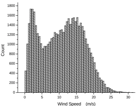
In this study, the wind speed data recorded in Khaf area, Khorasan province, Iran in 2007 and 2008, are used. Histogram for wind speed has been shown in Fig. 1.
The wind power values have been calculated based on the hourly average of wind speed data, using turbine power curve. Typical pitch-controlled WTG are considered in this study. No known standard distribution function can be fitted to the samples that have been plotted in Fig. 1. Using MCS and sampling from wind speed, wind power generation can be determined.
A piece-wise linear WTG power curve is represented in [21] and the wind generation is obtained based on the method described in [22]. In a wind farm, as the wind speed regime is assumed to be the same for all turbines, total generated power is obtained by aggregating the generations of all wind turbines.
0 5 10 15 20 25 30 0
200 400 600 800 1000 1200 1400 1600 1800
Cou
n
t
Wind Speed (m/s)
Fig. 1 Wind Speed Histogram for 52560 sample (sampling every 10 minutes in one year).
0.0 0.2 0.4 0.6 0.8 1.0
5000 10000 15000 20000 25000 30000 35000
System Loa
d
(KW)
Win Power Generation (pu)
Fig. 2 Scatter plot for Load Samples and Wind Power Generation shows their correlation.
3.3 Modeling Correlation Between Wind Power Generation and Load
The marginal distribution of the wind speed was shown in the previous section. The Scatter plot for the wind power generation and load samples is shown in Fig. 2. This figure indicates the correlation between the wind power generation and load with the correlation degree of 0.42. As it has been shown in the Fig. 2, wind power generation and system loads are not independent. If load level is identified, wind power generation is bounded according to their correlation.
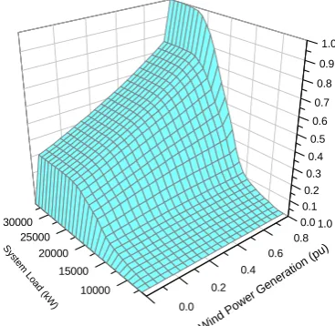
Joint Cumulative Mass Function (CMF) for wind power generation and load samples has been plotted in Fig. 3. As plotted in Fig. 3, for each level of system load there is a CMF for wind power generation. For a specified level of load, probability for wind power generation can be obtained based on follow:
(
)
(
)
w
Cap
0 w w 0 w w
p 0
prob L l , P p prob L l , P p
=
= ≤ =
∑
= = (18)0.0 0.2
0.4 0.6
0.8 1.0
10000 15000 20000 25000
30000 0.0
0.1 0.2 0.3 0.4 0.5 0.6 0.7 0.8 0.9 1.0
S yste
m L
oa d (kW
)
Wind
Pow
er G
ener
ation
(pu)
Fig. 3 Joint CMF for Load and Wind Power Generation.
0.0 0.2 0.4 0.6 0.8 1.0
0.0 0.1 0.2 0.3 0.4 0.5 0.6 0.7 0.8 0.9 1.0 1.1
Jo
in
t C
M
F
Wind Power Generation (pu) System Load in 10 MW
System Load in 15 MW System Load in 20 MW System Load in 30 MW
Fig. 4 Joint CMF versus Wind Power Generation
CMF for wind in a constant load (l0) is illustrated in
Fig. 4. In this figure, joint CMF has been plotted for wind power generation variations.
As it has been shown in Fig. 4, the CMF in each system level is different. Now corresponding to each selected load level, conditional CMF for wind power generation is obtained. Well-known Bayes Theorem for conditional probability is stated as follow:
(
)
(
)
(
)
w w
w w
prob L l, P p
prob P p L l prob L l
= =
= = = × = (19)
Equation (18) can be rewritten by conditional probability as follow:
(
)
(
)
(
)
w
0 w w
Cap
w w 0 0
p 0
prob L l , P p
prob P p L l prob L l
=
= ≤
=
∑
= = × = (20)Probability of load is the value of CMF in the maximum wind power generation:
0.2 0.4 0.6 0.8 1.0
0 100 200 300 400 500 600
Co
unt
Output Power (pu)
Wind Generation in Base Load Wind Generation in High Load
Fig. 5 Output Power for an instance Wind Turbine.
(
)
(
)
w
0 w w 0
p
C prob L l= = =
∑
prob P =p L l= (21)C is depended on the load value. So:
(
)
(
)
w
Cap
0 w w w w 0
p 0
Pr L l , P p C Pr P p L l
=
= ≤ = ×
∑
= = (22)Hence, the probability of wind power generation varies between 0 and C at each specified level of load. The inverse CMF method can be used to generate Wind power generation samples [22]. Uniform variables have been generated on the interval [0 C].
Using inverse CMF, a wind power generation sample has been generated corresponding to each variable. The resulting value follows the wind distribution for a constant level of load. Wind generation distribution has been easily achieved based on wind power generation samples. Histogram for wind generation in base load (10 MW) and high load (30 MW) has been shown in Fig. 5.
4 Simulation Results
The proposed method is applied to the IEEE 118-bus test system for the evaluation. IEEE 118-bus system consists of 186 branches. IEEE 118-bus test system has 3 different zones. Peak load is 4242 MW. The transmission capacity limits are not given in the basic system data, thus the MVA limits for branches are set to 500.
4.1 Results Verification
In presented method, the load flow is assumed to be DC. In this section, the result of presented method is compared with the ATC values that have been obtained from DC load flow. To analyzing the effect of the assumption, a Continuation Power Flow (CPF), method is used to calculate the ATC, based on DC power flow (DC-PF). In CPF method, calculation is repeated for each increment in load at the sink bus and generation in source bus, till any line capacity limits has been over-ridded [18]. Calculation time depends on the step size that has been selected to search for the answer.
Table 1 Comparison of ATC Values (MW) for IEEE 118-bus. Bus Number Proposed Method CPF method
From To (MW) (MW)
58 17 792.06 793
90 17 801.46 802
58 49 928.23 929
90 49 810.27 811
49 58 939.38 940
90 58 752.67 753
49 90 717.8 718
58 90 667.77 668
17 90 889.09 890
Table 2 Calculation Time for ATC Value.
Bus Number Proposed Method CPF method
From To (sec.) (sec.)
58 17 1.74 2338.7
90 17 1.47 1887.0
58 49 1.42 3237.3
90 49 1.55 2708.5
49 58 1.54 3269.8
90 58 1.64 2679.4
49 90 1.70 1484.3
58 90 1.51 1338.6
Table 1 shows the comparison between result that is obtained from presented method and CPF method for IEEE 118 bus test system. ATC has been calculated for 8 different cases. In all cases, there is no WTG and load is half of peak load. Results are obtained from proposed method is matched with DC-PF results.
In CPF method, calculation has been started from 200 MW and procedure has been discretized in 1 MW steps to decrease the time of calculation. It is worth noting, ATC distribution is obtained, using CPF method by heavy computational burden such that the distribution cannot be achieved in rational time. While this drawback is eliminated using the proposed method. Table 2 shows the calculation time for 1000 samples in selected cases using a 2.13 GHz Intel Core i3 processor with 4 GB of RAM.
As Table 2 shows, calculation time for proposed method is much lower than CPF method. Hence CPF method is not suitable for large systems [23]. Proposed method calculation time is independent from case study. In CPF method calculation time increase when the ATC value is high.
4.2 Wind Power Penetration
In this section, it has considered that the 4 wind turbine installed in 4 different sites in the system. Different scenario can be defined based on load level, wind capacity penetration and selected paths for transmission power. The aggregated wind generation capacity is considered to increase from 5 % to 10 % of system peak load. Wind generations added to buses number 59, 61, 65 and 66.
Table 3 Mean Value and Standard Deviation for ATC from
Bus 17 to Bus 90.
Aggregated Wind Generation Capacity
5% 10% Mean
Value Deviation Standard Mean Value Deviation Standard
Syste
m
Load Base 716.76 82.03 654.93 183.47
Medium 661.26 98.78 578.26 194.99
High 548.96 104.47 368.14 201.16
Table 4 Mean Value and Standard Deviation for ATC from
Bus 90 to Bus 49.
Aggregated Wind Generation Capacity
5% 10% Mean
Value Deviation Standard Value Mean DeviationStandard
Syste
m
Load Base 819.25 44.80 832.79 62.03
Medium 833.01 34.64 854.22 51.56
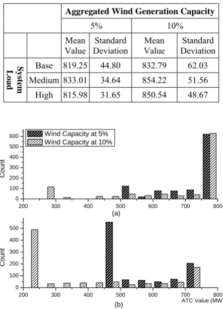
High 815.98 31.65 850.54 48.67
200 300 400 500 600 700 800
0 100 200 300 400 500 600
Co
un
t
Wind Capacity at 5% Wind Capacity at 10%
200 300 400 500 600 700 800
0 100 200 300 400 500
(a)
Co
unt
ATC Value (MW)
(b)
Fig. 6 ATC distribution for Table 3 scenarios: a) Low Load b)
High Load.
All sites have equal size and Capacity of these generation set 25 % of aggregated wind power. ATC for two different paths have been calculated.
As it has shown in Tables 3 and 4, wind generation effect on ATC is differed base on case study. Both increase and decrease of ATC value can be observed. In Table 3, the results show negative effect of wind generation increment on system ATC value whereas in Table 4, ATC value increase with wind generation.
The ATC distribution for 4 scenarios has been plotted in Fig. 6. According to this figure, ATC distribution is similar to wind generation distribution as
it has been expected according to Eq. (16). Beside wind generation distribution load level determines, ATC distribution trend.
Although, wind generation effect in low load scenarios is smaller than its effect on high load scenarios. This can be explained by the correlation between wind and load that mentioned in section 2.
According to the results, variance for these cases increases when the wind generation capacity is high. Decrement in mean value as well as increment in standard deviation indicate negative effect of WTG on the system ATC. This is clear on the high load scenario in Fig. 6(b). On the other hand, positive impact of ATC can be seen in Table 4, while the mean value increase in medium load and the standard deviation decrease. For generation and transmission expansion planning, experts have to consider this subject in placement and sizing of WTGs. The results may differ from case to case but presented method can be applied for all system, which is time efficient and has low computational cost.
5 Conclusion
In this paper, a new formulation for the ATC problem was proposed to solve the problem analytically. In the proposed formulation, ATC problem was converted as a linear one that decreases the calculation time. A proof presented for the ATC calculation using the PDTF and linear combination of the injected powers. With the aid of the proposed method, the Monte Carlo Simulation time significantly decreases. Hence, the proposed method is suitable for modeling different sources of uncertainty. A numerical algorithm based on inverse CMF method has been used to decompose wind power generation according to its dependency to load level. The numerical results show the influence of wind farm location on ATC value. If wind farms locate in adequate place, additional transmission capacity can be released. Conversely, a wind farm in inadequate bus occupies line transmission capacity. Proposed equation shows the effect of network structure, wind capacity and dependency to load level on ATC value. Analytical result has been confirmed with simulated scenarios.
Appendix List of Symbols
Ptrans,ij Power transfer between bus i and j
Pbranch,k Power transmitted in like k
branch,k
P Upper thermal limit of branch k Nl Number of branches
Pbus Bus injected power matrix
Xmn The impedance value for line k between bus m and n
Θ Bus angle vector
B Susceptance matrix
( )
Pbus old Base load matrix for busesPwind Wind power generation matrix
L Load variable
L Load level
Pw Wind generation variable
pw Wind generation level
Cap Wind turbine capacity C Probability for marginal loads
References
[1] A. Leite da Silva, J. Lima and G. Anders, “Available Transmission Capability - Sell Firm or Interruptible?”, IEEE Transactions on Power Systems, Vol. 14, No. 4, pp. 1299-1305, 1999. [2] R. Christie, B. Wollenberg and I. Wangensteen,
“Transmission Management in the Deregulated Environment”, Proceedings of the IEEE, Vol. 88, No. 2, pp. 170-195, 2000.
[3] C. Wang, X. Wang and P. Zhang, “Fast Calculation of Probabilistic TTC with Static Voltage Stability Constraint”, IEEE Power Engineering Society General Meeting, Tampa, FL, 2007.
[4] G. C. Ejebe, J. G. Waight, M. Santos-Nieto and W. F. Tinney, “Fast Calculation of Linear Availible Transfer Capability”, IEEE Transactions on Power Systems, Vol. 15, No. 3, pp. 1112-1116, 2000.
[5] J. Kumar and A. Kumar, “Multi-transactions ATC Determination using PTDF based Approach in Deregulated Markets”, Annual IEEE India Conference (INDICON), pp. 1-6, 2011.
[6] A. Khairuddin and N. A. Bakar, “ATC Determination Incorporating Wind Generation”, International Power Engineering and Optimization Conference, pp. 501-506, Langkawi, Malysia, 2013.
[7] B. Alberto, C. Bovo, M. Delfanti, M. Merlo and M. S. Pasquadibisceglie, “A Monte Carlo Approach for TTC Evaluation”, IEEE Transactions on Power Systems, Vol. 22, No. 2, pp. 735-743, 2007.
[8] H. Falaghi, M. Ramezani, C. Singh and M. R. Haghifam, “Probabilistic Assessment of TTC in Power Systems Including Wind Power Generation”, IEEE Systems Journal, Vol. 6, No. 1, pp. 181-190, 2012.
[9] A. Leite da Silva, J. de Carvalho Costa, L. da Fonseca Manso and G. Anders, “Transmission capacity: availability, maximum transfer and reliability”, IEEE Transactions on Power Systems, Vol. 17, No. 3, pp. 843-849, 2002.
[10] H. Falaghi, M. Ramezani, C. Singh and M.-R. Haghifam, “Role of Clustering in the Probabilistic Evaluation of TTC in Power Systems Including
Wind Power Generation”, IEEE Transactions on Power Systems, Vol. 24, No. 2, pp. 849-858, 2009.
[11] N. Paensuwan and A. Yokoyama, “Probabilistic TTC of a Power System Integrated with Wind Generation Systems”, The International Conference on Electrical Engineering, 2009.
[12] N. Paensuwan and A. Yokoyama, “Risk-Based Dynamic TTC Calculation in a Deregulated Power System with a Large Penetration of Wind Power Generation”, Integration of Wide-Scale Renewable Resources Into the Power Delivery System, CIGRE/IEEE PES Joint Symposium, Calgary, 2009.
[13] K. Audomvongseree and A. Yokoyama, “Risk based TTC Evaluation by Probabilistic Method”, IEEE Power Tech. Conference, Bologna, Italy, Vol. 2, p. 6, 2003.
[14] L. Gang, Ch. Jinfu, C. Defu, Sh. Dongyuan and D. Xianzhong, “Probabilistic assessment of available transfer capability considering spatial correlation in wind power integrated system”, IET Generation, Transmission & Distribution, Vol. 7, No. 12, pp. 1527,1535, 2013.
[15] E. Shayesteh, B. F. Hobbs, L. Soder and M. Amelin, “ATC-Based System Reduction for Planning Power Systems With Correlated Wind and Loads”, IEEE Transactions on Power Systems, Vol. 30 , No. 1, pp. 429-438, 2015. [16] Ch. Hsiao-Dong, and H. Sheng, “Available
Delivery Capability of General Distribution Networks With Renewables: Formulations and Solutions”, IEEE Transactions on Power Delivery, Vol. 30, No. 2, pp. 898-905. 2015.
[17] M. Khosravifard and M. Shaaban, “Risk‐based available transfer capability assessment including nondispatchable wind generation", International Transactions on Electrical Energy Systems, Vol. 25, No. 11, pp. 3169-3183, 2015.
[18] B. Michael, K. Trepper and Ch. Weber, “Impacts of renewables generation and demand patterns on net transfer capacity: implications for effectiveness of market splitting in Germany”, IET Generation, Transmission & Distribution, Vol. 9, No. 12, pp. 1510-1518, 2015.
[19] M. Asghari and H. Rajabi Mashhadi, Available Transfer Capacity Assessment in Deregulated Power System, A thesis in Persian, Ferdowsi University of Mashhad, 2009.
[20] A. J. Wood and B. F. Wollenberg, Power Generation, Operation, and Control, 2nd Edition, John Willey and Sons, 2012
[21] H. Valizadeh Haghi, M. Tavakoli Bina, M. Golkar and S. Moghaddas-Tafreshi, “Using Copulas for analysis of large datasets in
renewable distributed generation: PV and wind power integration in Iran”, Renewable Energy, Vol. 35, No. 9, pp. 1991-2000, 2010.
[22] S. Hagspiel, A. Papaemannouil, M. Schmid and G. Andersson, “Copula-based modeling of stochastic wind power in Europe and implications for the Swiss power grid”, Applied Energy, Vol. 96, pp. 33-44, 2011.
[23] T. Niknam, H. R. Massrur and B. Bahmani Firouzi, “Stochastic generation scheduling considering wind power generators”, Journal of Renewable and Sustainable Energy, Vol. 4, No. 6, pp. 212-219, 2012.
[24] M.-K. Kim, D.-H. Kim, Y. T. Yoon, S.-S. Lee and J.-K. Park, “Determination of Available Transfer Capability Using Continuation Power Flow with Fuzzy Set Theory”, IEEE Power Engineering Society General Meeting, pp. 1-7, 2007.
Mohammad Azim Armin was born in
Bandar Abbas, Iran, in 1981. He received the B.Sc. degree from Chamran University, Ahvaz, Iran, in 2004 and the M.Sc. degree from Ferdowsi University of Mashhad, Mashhad, Iran, in 2007, both in electrical engineering. He is Ph.D. student in Ferdowsi University of Mashhad, Mashhad. His areas of interest include renewable power generation, system reliability evaluation and probabilistic load flow.
Habib Rajabi Mashhadi was born in
Mashhad, Iran, in 1967. He received the B.Sc. and M.Sc. degrees with honor from the Ferdowsi University of Mashhad, both in electrical engineering, and the Ph.D. degree from the Department of Electrical and Computer Engineering of Tehran University, Tehran, Iran, under joint cooperation of Aachen University of Technology, Germany, in 2002. He is as Associate Professor of electrical engineering at Ferdowsi University of Mashhad. His research interests are power system operation and planning, power system economics, and biological computation.