A Stochastic Model For Protrusion Activity

Muhammad DAUHOO, Laurent DUMAS, Pierre GABRIEL and Pauline LAFITTE

A STOCHASTIC MODEL FOR PROTRUSION ACTIVITY

Christ`

ele Etchegaray

and Nicolas Meunier

Abstract. In this work we approach cell migration under a large-scale assumption, so that the system reduces to a particle in motion. Unlike classical particle models, the cell displacement results from its internal activity: the cell velocity is a function of the (discrete) protrusive forces exerted by filopodia on the substrate. Cell polarisation ability is modeled in the feedback that the cell motion exerts on the protrusion rates: faster cells form preferentially protrusions in the direction of motion. By using the mathematical framework of structured population processes previously developed to study population dynamics [4], we introduce rigorously the mathematical model and we derive some of its fundamental properties. We perform numerical simulations on this model showing that different types of trajectories may be obtained: Brownian-like, persistent, or intermittent when the cell switches between both previous regimes. We find back the trajectories usually described in the literature for cell migration.

1.

Introduction

Cell migration is a fundamental process involved in physiological and pathological phenomena such as the immune response, morphogenesis, but also the development of metastasis from a tumor [1, 5]. To ensure these functions, cells have a highly complex out-of-equilibrium internal organization where multiscale reactions occur among polymers and molecules, leading to unpredictable macroscopic behaviours.

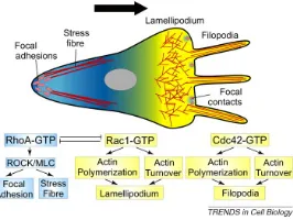
In the case of cell crawling, cells spread on an adhesive substrate, and form extensions also called protrusions. Then, molecular adhesion complexes grow and ensure a mechanical connection between protrusions and the substrate, by which forces are transmitted and lead to a displacement. Protrusions of a crawling cell can be divided in two types: lamellipodiaare wide and flat and fluctuate continuously, whilefilopodiaare long finger-like extensions able to grow further and probe the substrate.

It has been observed that cells protrusive activity fluctuates a lot, and that these fluctuations are responsible for the long-term characteristics of trajectories [2]. Cell trajectories can be very different even for a single cell type: some do not explore the environment, while others have a much more efficient displacement. It is of interest to try to capture this diversity in a mathematical model.

Existing stochastic models for cell trajectories are either Random Walks, L´evy flights or Active Brownian Particle models [9]. In these models, key-features of the motion are quantified, such as the mean persistence time, or the stationary distribution of the particle’s velocity [9]. However, the dynamics is macroscopic and

∗_... ∗∗ _...

1 _{MAP5, CNRS UMR 8145, Universit´e Paris Descartes, 45 rue des Saints P`eres 75006 Paris, France.}

e-mail:[email protected]

2 _{MAP5, CNRS UMR 8145, Universit´e Paris Descartes, 45 rue des Saints P`eres 75006 Paris, France.}

e-mail:[email protected]

c

EDP Sciences, SMAI 2018

Figure 1. Scheme of a polarised crawling cell: protrusive structures at the front (lamel-lipodium, filopodia), and contractile fibers at the back. The asymmetric activity combines with an asymmetric repartition of molecular regulators organized in feedback loops. Source: [7]

processes such as polarisation are taken into account by an arbitrary positive feedback at the scale of the trajectory. In this work, we present a 2D stochastic particle model for cell trajectories based on the filopodial activity, able to reproduce the diversity of trajectories observed.

2.

Model construction

We choose space and time scales large enough so that the cell is described as an active particle (its center of mass). Cell shape and intracellular dynamics are therefore considered at the cell scale. We define now the velocity model that is based on force equilibrium.

2.1.

Velocity model

At each time, the cell velocity writesV~t, and its polar coordinates (vt, θt). The crawling of cells on an adhesive

substrate occurs at very small scales. Indeed, cells sizes are of the order of 1−10µm, while their speeds ranges at the scale of µm s−1_{. Therefore, inertia is negligible for this system (see more precise justifications of the} low Reynolds number setting in e.g [10]), and Newton’s second law of motion reduces to instantaneous force equilibrium: at all timet≥0,

X_~

Fext(t) =~0.

The cell being an active system, macroscopic forces that apply can be either passive or active. In this case appear

→ a passive force: the friction force exerted by the substrate on the cell due to motion, that writes

~

f =−γ ~Vt, withγ the global friction coefficient,

→ active forces related to the protrusion process. Indeed, a complex internal activity gives rise to forces in the body of the cell. Filopodial protrusions can be considered as good readouts [2]. As a consequence, in the following, only filopodial forces will be considered. Note that at this scale, the formation of filopodia is discontinuous in time.

Combining these information, we get:

γ ~Vt= Nt

X

i=1 ~

Fi(t), (1)

whereNtis the number of filopodia adhering on the substrate at timet, and (F~i(t))ithe filopodial forces. The

cell motion is then entirely described by the protrusions.

Now, denotingθi=arg(F~i), one can write

~ Fi(t) =

cos(θi)

sin(θi)

.

Modelling cell motion then accounts to modelling the time evolution of the filopodial population in terms of individual orientation.

2.2.

Protrusion model

Each filopodium is characterized by a quantitative parameter, its orientationθ∈[0,2π). Therefore, we use a measure valued process for the stochastic evolution of the set of filopodia, as in ecological population models [4]. Let us denote MF(χ) the set of positive finite measures on χ = [0,2π], equipped with the weak topology. Notice that asχis compact, weak and vague topologies onMF(χ) coincide. WriteMfor the subset ofMF(χ) composed of all finite point measures. Then, a filopodium of orientation θis described by a Dirac measure δθ

onχ, and the whole population by

νt= Nt

X

i=1

δθi ∈ M.

For any measurable function f onχ and anyµ∈ MF(χ), we have < µ, f >=R

χf(θ)µ(dθ). In particular,

< νt, f >=P Nt

i=1f(θi), and the population size corresponds to Nt =< νt,1 >. A simple way to express the

velocity equation (1) together with hypothesis (2.1) is to write

γ ~Vt=

< νt,cos>

< νt,sin>

.

The cell motion is entirely described by a measure-valued markovian jump process (νt)t, as in adaptive

stuctured population models. We describe now the different events arising.

• The basic dynamics arising is theisotropic appearanceof filopodia. It is responsible for the sponta-neous activity that is observed experimentally. We writecfor the creation rate.

• Each filopodium ends up disappearing: the disappearance ordeathrate is denoted bydconstant.

• Polarisationis characterized by a morphological and functional asymmetry visible both on cell shape and at the microscopic scale [3, 8]. Here, we use the mesoscopic scale of the model to account for polarisation by its feedback on the protrusive activity. Two phenomena have to be distinguished:

→ The formation of a protrusion is induced by several microscopic regulators and generates a local positive feedback on the protrusive machinery. Following that, we assume that each filopodium is able toreproduce. Denoter(θi, νt) the individual reproduction rate of a filopodium of orientation

θi.

→ Polarisation is also reinforced by intracellular actin flows, (see [6]). In particular, faster actin flows favor the formation of protrusions in a single stable configuration. Denote~ufor the space-averaged actin flow velocity over the cell. As actin flows are inwardly directed, −~ucharacterizes the reinforced direction for protrusions. Moreover, we know thatV~ =−1

α~u, where

1

α depends on

the cell type and the experimental setting. Therefore, we consider a positive coupling between the reproduction rate and−~u=α~V, imposing a global feedback.

0.2 0.4

0.6

30

210

60

240 90

270 120

300 150

330

180 0

0.2 0.4

0.6

30

210

60

240 90

270 120

300 150

330

180 0

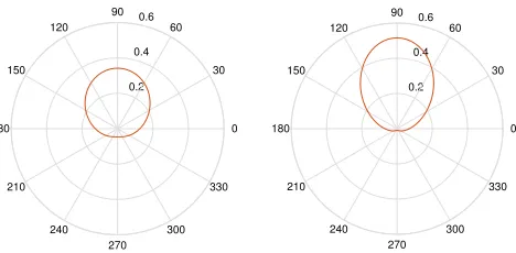
Figure 2. Circular distribution forθt= π₂,κ= 1 (left) andκ= 2 (right).

For simplicity, we assume that at each reproduction event, the mutation probabilityµis constant. In the case of a mutant new protrusion, its orientation is determined following a probability distribution

g(z;θi) assumed centered in the parent’s orientationθi, with a constant variance.

The possible events are summed up in the following graph: Creation (global)

c

Clone Reproduction (individual) % 1−µ

r(θi, ν) &

Mutation −→ Choice ofθ

Death (individual) µ g(z;θi)

d

Let us comment on the mathematical features of the model. In the case of no interaction between indi-viduals, or global feedback, the process (Nt)t simply follows an immigration, birth and death dynamics, and

mathematical information can be derived. In particular, the branching property still holds. This is no longer the case when adding interactions. For example, if the interaction relies on Vt, then knowing only Nt is not

sufficient and one has to know about the structured quantities (Nθ1_{, N}θ2_{, ...) at all time.}

A choice of reproduction rate and mutation law

As protrusions are located on [0,2π), it is natural to consider reproduction rates as circular functions. We chose a reproduction function that is positively correlated to α~Vt to account for polarisation. The idea is to

have a function centered inθt the direction of motion, that gets sharper with increasingvt.

We choose a reproduction rate as a multiple of a circular normal distribution density written

f(θi;V~t) =

1

2πI0(κ(||V~t||))

exp(κ(||V~t||) cos(θi−arg(V~t))),

with κ(||V~t||)≥ 0 a non decreasing shape parameter, and I0 the 0-order modified Bessel function of the first kind. Therefore, we denoter(θ, νs) =r∗f(θ;θt, κ).

The mutation law is a circular normal distribution on [0,2π) of density g(z;θi), centered in θi and with a

constant shape parameter (resp. variance) κ(resp. σ2).

3.

Mathematical properties

From now on, we will use the notationC for any constant, that will change from line to line.

We introduce here a stochastic differential equation for (νt)tdriven by Point Poisson Measures. We will show

In order to pick a specific individual in the population, we have to be able to order them or their trait. Indeed, from the n-uplet (θ1, ..., θN), one can recoverν =P

N

i=1δθi, but fromν it is only possible to know{θ1, ..., θN}.

Definition 3.1. Let us define the function

H = (H1_{, ..., H}k_{, ...) : M −→ (χ)}N∗

ν =

n

X

i=1

δθi 7−→ (θσ(1), ..., θσ(n), ...),

with θσ(1) θσ(2) ...θσ(n), for an arbitrary order . Now, an individual can be picked by its label i, and the corresponding trait writesHi_{(ν) =θ}

σ(i).

Let (Ω,F,P) be a probability space, and n(di) the counting measure on N∗. We introduce the following

objects:

• ν0∈ Mthe finite point measure describing the initial population, eventually equal to the null measure. It can be chosen stochastic as soon asE[< ν0,1>]<+∞.

• M0(ds,dθ,du) a Poisson Point Measure on [0,+∞)×χ×R+, of intensity measure dsdθdu,

• M1(ds,di,du) and M3(ds,di,du) Poisson Point Measures on [0,+∞)×N∗×R+, both of intensity measure ds n(di) du,

• M2(ds,di,dθ,du) a Poisson Point Measure on [0,+∞)×N∗×χ×R+, of intensity measure dsn(di)dθdu. The Poisson Measures are independent. Finally, (Ft)t≥0 denotes the canonical filtration generated by these objects. Let us construct the (Ft)t≥0-adapted process (νt)t≥0 as the solution of the following SDE:∀t≥0,

νt = ν0

+ Z t

0 Z

χ×R+

δθ 1u≤c

2π M0(ds,dθ,du)

+ Z t

0 Z

N∗×R+

δHi_(ν

s) 1i≤Ns 1u≤(1−µ)r(Hi(νs),νs) M1(ds,di,du)

+ Z t

0 Z

N∗×χ×R+

δθ 1i≤Ns 1u≤µr(Hi(νs),νs)g(θ;Hi(νs))) M2(ds,di,dθ,du)

−

Z t

0 Z

N∗×R+

δHi_(ν

s) 1i≤Ns 1u≤d M3(ds,di,du).

(2)

In this equation, each term describes a different event. The Poisson Point Measures generate atoms homo-geneously in time. However, the dynamics we want to describe follows state-dependent rates. Hence, we use indicator functions to keep only some of the events in order to get the wanted rates. Then, the Dirac measures correspond to the individuals added to or removed from the population.

Hypothesis 3.2. The reproduction rate is a bounded function:

∃r >0 such that ∀ν∈ M, ∀(θ, ν)∈χ× M, 0≤r(θ, ν)≤r.

3.1.

Existence and uniqueness

In this part let us prove existence and uniqueness of a solution for equation (2). Recall thatNt=< νt,1>.

Proposition 3.3. Assume the boundedness of the reproduction rate (hypothesis 3.2), and thatE[N0] <+∞. Then, the two following properties hold.

(1) There exists a solution ν∈D(R+,M(χ))of equation (2) such that

∀T >0, E

"

sup

t∈[0,T] Nt

#

<E[N0]erT+ c r(e

(2) There is strong (pathwise) uniqueness of the solution.

Proof of 3.3. The proof is similar to prop. 2.2.5 and 2.2.6 in [4].

(1) LetT0= 0, and t∈R+. Then, the global jump rate ofνtis smaller thanc+ (r+d)Nt. Hence one can

P−a.sdefine the sequence (Tk)k∈N∗ of jumping times, as well asT∞:= limk→+∞Tk.

Now, by construction, it is _P−a.s possible to build ”step-by-step” a solution of equation (2) on [0, T∞[. Showing existence of a solution (νt)t∈R+ ∈ D(R+,M(χ)) amounts to showing that P−a.s,

T∞ = +∞. That is equivalent to saying that there cannot be an infinite number of jumps in a finite

time interval.

• First, we show the control property (3). For n > 0 define the sequence of stopping times (τn)n

by

τn = inf

t≥0{Nt≥n}.

→ Let us show that (τn)n≥0is a sequence of stopping times for (Ft)t. Denoteσt=σ(νs, 0≤

s≤t) the σ-algebra generated by {νs, 0 ≤s ≤t}. Then ∀t ≥0, σt⊆ Ft. For (n, m)∈ (N∗)2,

notice that

{τn ≤m}={inf{t≥0, hνt,1i ≥n} ≤m} ∈σm⊆ Fm,

and (τn)n≥0is indeed a sequence of stopping times.

→ Now, we prove that for all T < +∞, the quantity _Ehsup_{t∈[0,T∧τn]}Nt

i

is bounded

∀n≥0.

Fort∈R+, using equation (2) and dropping the non-positive term, one has

Nt∧τn = < νt∧τn,1>≤N0+ Z t∧τn

0 Z

χ×R+

1u≤cM0(ds,dθ,du)

+

Z t∧τn

0 Z

N∗×R+

1i≤Ns1u≤(1−µ)r(Hi(νs),νs)M1(ds,di,du)

+

Z t∧τn

0 Z

N∗×χ×R+

1i≤Ns1u≤µr(Hi_(ν

s),νs)g(θ;Hi(νs))M2(ds,di,dθ,du).

As each integrand is positive, bounded, and integrable with respect to the intensity measure, taking the expectation and using the Fubini theorem, we can write

E

"

sup

t∈[0,T∧τN] Nt

#

≤ E[N0] +E

" Z T∧τN

0

c+

Nt

X

i=1

r(θi, νt)

!

dt

#

≤ E[N0] +cT+r Z T

0

E

"

sup

s∈[0,t∧τN]

Ns

#

dt

leading to theT-dependent bound using the Gronwall inequality.

→ Let us prove that P−a.s, limn→+∞τn = +∞. If this wasn’t the case, there would exist

M <+∞and a set AM ⊂Ω such thatP(AM)>0, and∀ω∈AM, limn→+∞τn(ω)< M. By the

Markov inequality,∀T > M,

E

"

sup

t∈[0,T∧τn] Nt

#

≥n_P sup

t∈[0,T∧τn] Nt≥n

!

| {z }

≥P(AM)>0

which is in contradiction with equation (4).

→ Property (3) is proved by the Fatou lemma:

E

"

sup

t∈[0,T] Nt

#

=E

"

lim inf

n→+∞_t∈[0sup_,T∧τ

n]

Nt

#

≤lim inf

n→+∞E

"

sup

t∈[0,T∧τn]

Nt

#

≤E[N0]erT + c r e

rT ₋₁

<+∞.

• Now, let us show that _P−a.s, T∞= +∞. If this is not the case, then there existsM <+∞ and a setA_M ⊂Ω such thatP(AM)>0 and∀w∈AM,T∞(ω)< M. Moreover, if the assertion

∀ω∈A_M, lim

k→+∞NTk(ω) = +∞, (4)

is true, then we would have

∀N >0, ∀ω∈A_M, τN(ω)≤M ,

which contradicts limn→+∞τn = +∞. As a consequence, if we prove (4), the proposition is proved.

If (4) is not true, there would existN0>0 and a setB ⊂A_M such thatP(B)>0 and

∀ω∈B, ∀k∈N, NTk(ω)< N0.

Then,∀ω ∈B, (Tk(ω))k can be seen as the subsequence of a sequence of jumping times (Tk1(ω))k

of a Point Poisson Process of intensity c+ (r+d)N0. The only accumulation point of (T1

k(ω))k

being_P−a.s +∞, it contradicts the definition ofB, and proves (4).

(2) The sequence of jumping times (Tk)k∈N being already defined, we only have to show that (Tk, νTk)k∈N

are uniquely determined byD= (ν0, M0, M1, M2, M3) defined above. But this is clear by construction of the process.

3.2.

Markov property

Now, we can show that the solution (νt)t of equation (2) is a Markov process in the Skorohod space

D(R+,MF(χ)) of c`adl`ag finite measure-valued processes on χ. For that purpose, we introduce ∀ν ∈ M, Φ :M →Rmeasurable and bounded, the operator Ldefined by

LΦ(ν) = Z

χ

c

2π[Φ(ν+δθ)−Φ(ν)] dθ

+ Z

χ

(1−µ)r(θ, ν) [Φ(ν+δθ)−Φ(ν)]ν(dθ) (5)

+ Z

χ

µr(θ, ν) Z

χ

[Φ(ν+δz)−Φ(ν)]g(z;θ)dz ν(dθ)

+ Z

χ

d[Φ(ν−δθ)−Φ(ν)]ν(dθ).

Proposition 3.4. Take (νt)t≥0 the solution of equation (2) with E[< ν0,1 >] < +∞. Then, (νt)t≥0 is a Markovian process of infinitesimal generatorL.

Proof of proposition 3.4. The process (νt)t≥0 ∈ D(R+,M(χ)) is markovian by construction. Now, let N0 < N <+∞, and consider again the stopping time τN. Let Φ :M →Rbe measurable and bounded. AsP−a.s

we can write

Φ(νt) = Φ(ν0) + X

s≤t

Φ(νs−+ (ν_s−ν_s−))−Φ(ν_s−), (6)

we have

Φ(νt∧τN) = Φ(ν0) +

Z t∧τN

0 Z

χ×R+

[Φ(νs−+δθ)−Φ(νs−)]1u≤c

2πM0(ds,dθ,du)

+

Z t∧τN

0 Z

N∗×R+

h

Φ(νs−+δ_Hi_(ν

s−))−Φ(νs−)

i

1i≤N_s−1u≤(1−µ)r(Hi(ν_s−),ν_s−)M1(ds,di,du)

+

Z t∧τN

0 Z

N∗×χ×R+

[Φ(νs−+δ_z)−Φ(ν_s−)]1_i≤N

s−1u≤µr(Hi(νs−),νs−)g(z;Hi(νs))M2(ds,di,dz,du)

+

Z t∧τN

0 Z

N∗×R+

h

Φ(νs−−δ_Hi_(ν

s−))−Φ(νs−)

i

1i≤N_s−1u≤dM3(ds,di,du).

Again, as all integrands are bounded, we can take expectations to get

E[Φ(νt∧τN)] = E[Φ(ν0)] +E

Z t∧τN

0 Z

χ

[Φ(νs−+δ_θ)−Φ(ν_s−)]

c

2πdθds

+ E



 Z t∧τN

0

N_s− X

i=1 h

Φ(νs−+δ_Hi(ν_s−))−Φ(νs−) i

(1−µ)r(Hi(νs−), ν_s−)ds 



+ _E



 Z t∧τN

0

N_s− X

i=1

µr(Hi(νs−), ν_s−) Z

χ

[Φ(νs−+δ_z)−Φ(ν_s−)]g(z;Hi(ν_s))dzds 



+ E



 Z t∧τN

0

N_s− X

i=1 h

Φ(νs−−δ_Hi_(ν

s−))−Φ(νs−)

i

dds



,

=: _E[Φ(ν0)] +E[ψ(t∧τN, ν)].

On the one hand,∀t∈[0, T],

kψ(t∧τN, ν)k∞ ≤ 2T kΦk∞c+ 2T kΦk∞(1−µ)rN+ 2T kΦk∞µrN+ 2T kΦk∞dN

≤ CT kΦk∞(c+ (r+d)N)<+∞.

∂ψ

∂t(0, ν0) =

Z

χ

[Φ(ν0+δθ)−Φ(ν0)] c

2πdθ

+

N0

X

i=1

Φ(ν0+δHi_(ν

0))−Φ(ν0)

(1−µ)r(Hi(ν0), ν0)

+

N0

X

i=1

µr(Hi(ν0), ν0) Z

χ

[Φ(ν0+δz)−Φ(ν0)]g(z;Hi(ν0))dz

+

N0

X

i=1

Φ(ν0−δHi_(ν

0))−Φ(ν0)

d .

Moreover,k ∂ψ_∂t(0, ν0)k≤CkΦk∞(c+N0(r+d)). Now,

Lφ(ν0) :=

∂E[φ(νt)]

∂t _t=0 = Z χ

[Φ(ν0+δθ)−Φ(ν0)] c

2πdθ+

N0

X

i=1

Φ(ν0+δHi_(ν

0))−Φ(ν0)

(1−µ)r(Hi(ν0), ν0)

+

N0

X

i=1

µr(Hi(ν0), ν0) Z

χ

[Φ(ν0+δz)−Φ(ν0)]g(z;Hi(ν0))dz

+

N0

X

i=1

Φ(ν0−δHi_(ν

0))−Φ(ν0)

d,

or equivalently

Lφ(ν0) = Z

χ

[Φ(ν0+δθ)−Φ(ν0)] c

2πdθ+

N0

X

i=1

Φ(ν0+δHi_(ν

0))−Φ(ν0)

r(Hi(ν0), ν0)

+

N0

X

i=1

Φ(ν0−δHi_(ν0))−Φ(ν0)d

+µ

N0

X

i=1

r(Hi(ν0), ν0) Z

χ

Φ(ν0+δz)g(z;Hi(ν0))dz−Φ(ν0+δHi(ν0))

.

4.

Numerical simulations

The construction of the process (νt)tfurnishes directly an algorithm for simulations. We proceed as follows:

start with the population measureνk at timetk, for a particle located atXk.

Time of next event: letτ =c+< νk, r+d > denote the global jump rate of the process. Then, the

time of the next event writestk+1:=tk+ ∆t, where

∆t∼Exp(τ).

Nature of the event: what happens at timetk+1 is determined as follows:

• reproduction of the protrusion numberioccurs with probability r(Hi(νk),νk)

τ . Then,

→ with probability (1−µ), the new protrusion has orientation Hi_(ν k),

→ with probabilityµ, its orientation is chosen with the realization of a random variable having a probability density g(·;Hi_(ν

k), νk). • protrusion numberidisappears with probability d

τ.

The measureνk+1 is then obtained fromνk and the information of the event occuring at timetk+1. Updates: the particle’s new position is

Xk+1=Xk+ ∆t Vk,

whileVk+1 =_γ1

< νk+1,cos> < νk+1,sin>

.

One only has to start again to get a trajectory over time.

4.1.

Results

References

[1] A. Aman and T. Piotrowski,Cell migration during morphogenesis, Developmental biology, 341 (2010), pp. 20–33. [2] D. Caballero, R. Voituriez, and D. Riveline,Protrusion fluctuations direct cell motion, Biophys J, 107 (2014), pp. 34–42. [3] V. Calvez, R. Hawkins, N. Meunier, and R. Voituriez,Analysis of a nonlocal model for spontaneous cell polarization,

SIAM Journal on Applied Mathematics, 72 (2012), pp. 594–622.

[4] N. Fournier and S. M´el´eard, A microscopic probabilistic description of a locally regulated population and macroscopic approximations, The Annals of Applied Probability, 14 (2004), pp. 1880–1919.

[5] P. Friedl and K. Wolf,Tumour-cell invasion and migration: diversity and escape mechanisms, Nat Rev Cancer, 3 (2003), pp. 362–74.

[6] P. Maiuri, J.-F. Rupprecht, S. Wieser, V. Ruprecht, O. B´enichou, N. Carpi, M. Coppey, S. De Beco, N. Gov, C.-P. Heisenberg, C. Lage Crespo, F. Lautenschlaeger, M. Le Berre, A.-M. Lennon-Dumenil, M. Raab, H.-R. Thiam, M. Piel, M. Sixt, and R. Voituriez,Actin flows mediate a universal coupling between cell speed and cell persistence, Cell, 161 (2015), pp. 374–86.

[7] R. Mayor and C. Carmona-Fontaine,Keeping in touch with contact inhibition of locomotion, Trends in cell biology, 20 (2010), pp. 319–328.

[8] N. Muller, M. Piel, V. Calvez, R. Voituriez, J. Goncalves-Sa, C.-L. Guo, X. Jiang, A. Murray, and N. Meunier,A predictive model for yeast cell polarization in pheromone gradients., PLoS Computational Biology, (2016).

[9] P. Romanczuk, M. B¨ar, W. Ebeling, B. Lindner, and L. Schimansky-Geier,Active brownian particles. from individual to collective stochastic dynamics, Eur.Phys.J., (2012).

x

-0.6 -0.5 -0.4 -0.3 -0.2 -0.1 0 0.1 0.2

y

-0.3 -0.2 -0.1 0 0.1 0.2 0.3 0.4 0.5

α=0.1

α=1

α=10

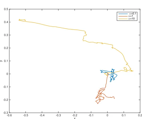
Figure 3. Numerical trajectories obtained for a varying polarisation parameterα. Parameters:

T = 100, ∆t= 10−4_{,c=d= 1,r= 0.95,γ= 90,µ= 0.2. Mutation concentration parameter} k= 10.

x

-0.15 -0.1 -0.05 0 0.05 0.1 0.15 0.2

y

-0.15 -0.1 -0.05 0 0.05 0.1 0.15 0.2 0.25 0.3

α=0.1

α=1

α=10

Figure 4. Numerical trajectories obtained for a varying polarisation parameterα. Parameters: