Journal of Computing and Security
http://www.jcomsec.org
An Optimal Traffic Distribution Method Supporting End-to-End
Delay Bound
Touraj Shabanian
a,∗
Massoud Reza Hashemi
aAhmad Askarian
aBehnaz Omoomi
baDepartment of Electrical and Computer Engineering , Isfahan University of Technology, Isfahan, Iran. bDepartment of Mathematical Science, Isfahan University of Technology, Isfahan, Iran.
A R T I C L E I N F O.
Article history:
Received:21 November 2012
Revised:31 July 2013
Accepted:14 September 2013
Published Online:20 December 2013
Keywords:
Traffic Distribution, Routing, Convex Optimization, Subgradient Method.
A B S T R A C T
Routing methods for optimal distribution of traffic in data networks that can also provide quality of service (QoS) for users is one of the challenges in recent years’ research on next generation networks. The major QoS requirement in most cases is an upper bound on end-to-end path delay. In multipath virtual circuit switched networks each session distributes its traffic among a set of available paths. If all possible paths are considered available, then the source’s decision on its traffic distribution can be considered as routing. A model of the routing function as a mathematical problem which distributes the input traffic over possible paths for each session is proposed here. A distributed and iterative algorithm which will keep the average end-to-end delay for individual paths below a required bound is introduced. This algorithm minimizes the total average delay of all packets in the network. The convergence of the algorithm is illustrated.
c
2014 JComSec. All rights reserved.
1
Introduction
Computer networks have evolved into a new genera-tion where a wide range of new services are provided to various network users [1]. For many of these new services, such as VOIP, IPTV, Network Games, etc, it is not sufficient just to transfer the information to the destination, but for the users’ satisfaction it is neces-sary to guarantee their required QoS as well. In this manner, the new services with arbitrary QoS
require-∗ Corresponding author.
Email addresses:[email protected](T. Shabanian),
hashemim@ cc.iut.ac.ir(M. R. Hashemi),
[email protected](A. Askarian),
[email protected](B. Omoomi)
ISSN: 2322-4460 c2014 JComSec. All rights reserved.
ments can be deployed in the network. Providing the QoS must be achieved by utilizing the least possible resources of the network such that the network can be optimized in terms of resource utilization [2]. Network optimization algorithms determine traffic distribution for a given traffic demand so that the optimum re-source utilization can be achieved. But the research results so far show that providing QoS in cases where routing is performed without paying attention to the QoS requirements is difficult. Therefore, considering the required QoS in the optimization algorithms and determining the routes accordingly is one of the chal-lenges of the next generation networks [3].
[4–8]. For an acceptable QoS it is required that the end-to-end delay is kept under a threshold level. Providing QoS is not an easy task in datagram networks. In new generation networks, virtual circuit switched networks such as MPLS is used to provide a better framework to implement QoS.
Most of the QoS provisioning algorithms in the literature exploit certain mechanisms to guarantee the delay for a given path. Nen Jin, et.al show that for providing QoS in a DiffServ network, the price per unit of traffic rate for each traffic class can be adjusted. They assume a given path for a user. The satisfaction of the user is modeled through a convex function of the traffic passing through that given path and the QoS level of the assigned traffic class [9]. In [5] QoS is proposed to be provided by adjusting the capacity allocated to each DiffServ class. The QoS measure is the exact proportion of the average delay of two different traffic classes. Each user’s traffic is routed through a predetermined path and depending on the amount of traffic of each class, the traffic over this path experiences a delay which is considered as its cost. In [6] a dynamic method is used to adjust the users’ traffic rate in a manner that a minimum rate and a maximum delay threshold are guaranteed. A predetermined path used for routing the traffic and its rate is determined by solving a convex optimization problem which satisfies the user’s delay requirements.
Most of the articles that study the traffic distribu-tion in virtual circuit switched networks assume a set of known paths for each source-destination pair. To simplify the problem, usually, a small set of paths is selected from all possible paths beforehand [10,11]. In the articles that find routes based on QoS require-ments, the QoS is mostly measured based onm pa-rameters. Each QoS parameter for a path is sum of the QoS parameters of its links. The links are modeled by an m-dimensional weight vectorW = (w1, ..., wm) the components of which represent the QoS parame-ters of links. Paths with QoS parameparame-ters lower than the threshold levels will satisfy the required QoS and can be selected. In this manner the QoS-based routing problem is modeled as a multi-constraint (optimal) problem. Since these problems are NP-hard, in most cases heuristic methods are adopted in solving them [3].
Here the objective is to introduce a scalable method in terms of the number of sessions, in order to dis-tribute the network’s traffic over available paths in a virtual circuit switched network that would min-imize the average delay for all packets as the total cost of the network, while guaranteeing a bounded end-to-end path delay as the users’ QoS requirement. The proposed method in this article is based on the
analysis of the traffic distribution problem with delay constraints. As a result, this problem is modeled as a constrained convex optimization problem and the routing algorithm is provided in accordance to the analytical solution of this problem.
In Section2an analytical model for distributing traf-fic is introduced where the traftraf-fic distribution is mod-eled as a constrained convex optimization problem. In Section3the Lagrangian dual method is adopted for solving this problem. An algorithm that can be real-ized in a data network based on the dual method is proposed here. In Subsection3.1the implementation method of the proposed algorithm in real networks is explained. In section4the simulation results are provided expressing that this proposed method con-verges and can achieve its objective in an effective manner. This article will be concluded in Section5. The analysis of the proposed model is provided in the AppendixA.
2
Traffic Distribution Model
The objective in common for all the routing algorithms is to determine the appropriate paths for carrying the users’ traffic from source to destination. All or part of each user’s traffic is assigned to each selected path; therefore, a direct output of a routing algorithm is the amount of traffic allocated to each path. In fact, routing can be modeled as a mathematical problem which determines the distribution of all sessions’ traffic over the network graph.
In this article source-destination pairs are assumed to be known and are presented by the setW. Each source-destination pair w ∈ W is considered as a session and its average input traffic is presented byrw. A data network is modeled as a stationary and directed graphG(A, V). The graph nodes, represented by set
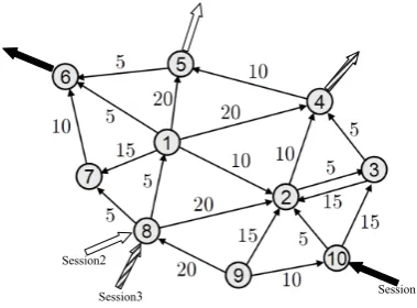
V model the network routers or gateways and graph links represented by setA, model the physical links between the routers. Some of the nodes of the graph are source or destination of the sessions in the network (Figure1). A session path is a set of links that connects the source of the session to its destination. The set of the paths of each session is calledPw. Thus the routing problem is similar to finding the distribution of each session’s traffic over its paths.
The parameters and notations which are used in the rest of this article are introduced in the following Nomenclature:
• W: The set of all existing sessions, whereNW shows the total number of these sessions
• P: The set of available paths of all sessionsw∈
W inG(A, V),whereNP shows the total number of these paths
Session2
Session3 Session1
Figure 1. A network graph with three sessions
• rw: Average traffic rate of sessionw
• xp: Traffic assigned to pathp∈P
• X: A vector ofNP components whosepth com-ponent is the assigned traffic to pathp,xp
• λp: The lagrangian multiplier according to the delay constraint of pathp
• Λ: A vector ofNP components whosepth com-ponent is theλp
• thp: The threshold level of average delay of pack-ets in pathp
• T h: A vector ofNP components whosepth com-ponent isthp
• fij: The flow crossing from link (i, j) ofG(A, V)
• hp(X): The cost function associated with pathp
• H(X): A vector of Np components whose pth component ishp(X)
• Dij(fij): The cost function associated with link (i, j)
Based on the above definitions the following rela-tions hold:
xp≥0 ∀p∈P (1)
X
p∈Pw
xp=rw ∀w∈W,∀p∈Pw (2)
fij =
X
p|(i,j)∈p
xp ∀(i, j)∈A (3)
hp(X) =
X
(i,j)∈p
Dij(fij) ∀p∈P (4)
If the average delay of the packets over a link is considered as the link’s cost function, Dij(fij), and the messages are delayed only by the links of the network, then (5) expresses the expected delay for all packets over the network [12]. Equation (5) indicates the average time that packets remain in the network and use network resources; thus, it can be considered as the overall system cost.
D= X (i,j)∈A
Dij(fij) (5)
Even in a virtual circuit network minimizing (5) can be a good objective for traffic distribution since it can improve network resource utilization [13,14]. In the virtual circuit switched networks, each session’s traffic is distributed among the available paths. By assuming a stable network and assuming that the traffic of the sessions is stationary, this problem is modeled and analyzed as the problem of distributing the average input traffic of each sessionrw, over the set of session’s pathsPw, which will result in the sessions’ path flowsxp, for all sessions. Thus,fij, the total flow of link (i, j), can be expressed by the different path flows. As a resultfij equals the sum of all path flows traversing link (i, j), (3). Here each session represents a customer. The expectation of each customer from the network is defined based on the customer’s traffic’s delay tolerance. In this case the customer will be satisfied if the average delay is bounded to a certain threshold. Therefore, considering the delay of each link as its cost is deemed to be appropriate. In this model the sum of the cost function of the links which compose a path, is considered as the path cost,hp(X), which is equal to the sum of the costs of the path’s links (4). Considering (5) as the overall cost function of the network and (4) as the customer cost, the limitation of which is required by the customers, the routing in the network can be modeled as Problem1.
Problem 1.
minimize D(X) = X (i,j)∈A
Dij(
X
p|ij∈p)
xp) (6)
X
p∈Pw
xp=rw ∀w∈W,∀p∈Pw (7)
xp≥0 ∀p∈P (8)
Problem 2.
minimizeD(X) = X (i,j)∈A
Dij(
X
p|ij∈p
xp)
X
p∈Pw
xp=rw ∀w∈W,∀p∈Pw
xp≥0 ∀p∈P
3
Solving The Problem
Usually the cost function Dij(fij) is expressed as a convex, non-decreasing, continuous and differentiable function; therefore, the path cost will have the above characteristics. Since the cost functionshp(X) are con-vex, Problem1is a constrained convex optimization problem [19,20], which can be solved using any of the existing methods, such as Projected Gradient, Interior Point, etc. But here the objective is to find a solu-tion that can also be implemented in real networks. In this regard the Lagrange dual problem is formu-lated and solved. In other words, since Problem1is a convex optimization problem the duality theorem is adopted in solving it. The fact that strong duality holds is presented in Proposition 1. Since there is a practical solution to solve Problem2[15], the dual problem is described using the Lagrange multipliers related to (9). Thus the Lagrangian is (10) where only constraint (9) is relaxed by introducing Lagrange mul-tiplierλp for each pathp∈P. The resultant partial dual function is Problem3[19].
L(X,Λ) =D(X) +X p∈P
λp.(hp(X)−thp) ∀Λ≥0 (10)
Problem 3.
q(Λ) = minimizeL(X,Λ)
X
p∈Pw
xp=rw ∀w∈W,∀p∈Pw
xp≥0 ∀p∈P
Considering Problem3as the dual function of Prob-lem1, the dual problem will be Problem4.
Problem 4.
maximize q(Λ)
λp≥0 ∀p∈P
As mentioned in Proposition2, the−q(Λ) is a con-vex function which is not necessarily differentiable in general, but it is sub-differentiable at all points. There-fore, Problem4can be solved iteratively by adopting the subgradient method [21]. In this method an initial
value is given to variable Λ, (Λ0), and in each itera-tion according to (11) a new value is calculated which will be closer to the optimum value.
Λk+1= [Λk+αk.gk]+ (11) To calculate the new value of Λ in the kth iteration, first a subgradient of function−q(Λ) called−gk is calculated at Λk, and then Λk+1is calculated by using (11) where,αk is a positive step size and ”+” denotes projection on the set R+. As result-4 indicates, in order to find a vectorgkthe traffic must be distributed based on Problem3solution according to Λ = Λk, denoted byX∗(Λk). In this case the deviation of the cost of a path from its thresholdthp, is equal to the associated component ofgk, (12).
gk=hp(X∗(Λk))−thp (12) Eventually, the iterative algorithm finds Λ∗which is the best solution for Problem4. Obviously in this iteration the input traffic is distributed similar to that of the path flows which are the solution of Problem3
for the amount of Λ = Λ∗. Since the conditions for strong duality exists according to Proposition1, this distribution will be the optimum solution of Problem1
as well. In the following section the proposed algorithm is explained. The convergence proof of this problem is presented in the AppendixA.
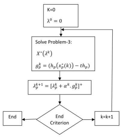
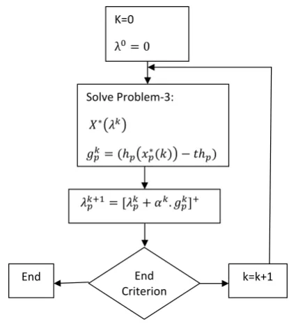
Algorithm Steps:
Step1: A feasible value is given to Λ. Since in Prob-lem4every Λ≥0 is acceptable, the Λ0= 0 is used as the initial value. In this step, the initial value ofqbest is 0.
Step2: In iteration k, Problem 3 must be solved based on the value of Λk, leading to the optimum valueq(Λk) and the optimum pointX∗(Λk). The com-ponents of this vector are represented byx∗p(Λk). In other words a mechanism must be used to determine path flows, for the optimal routing problem when (13) is considered as the cost function of each link. There-fore the Lagrange multipliers can be interpreted as the bottleneck indicators of the paths.
Dkij = (1 + X p|ij∈p
λkp).Dij(
X
p|ij∈p
x∗p(Λk)) (13)
Step3: In iterationk with respect to the value of
X∗(Λk) which is calculated in step2, the deviation of each path’s cost from the threshold level of the same path is calculated. Considering the Proposition3, the negative of this value can be considered as thepth
λ = 0 K=0
End Criterion
= (ℎ ∗( ) − ℎ )
Solve Problem-3:
∗
= [ + . ]
End k=k+1
Figure 2. The flowchart of flow distribution algorithm
−gkp. After calculating the deviation for all paths, the value of Λ for next iteration or Λk+1can be calculated using (11).
Step4: The value of qbest = max{qbest, q(Λk)}is calculated and k is increased by one. Then if the condition of ending the algorithm is met, the algorithm terminates, otherwise, it goes back to step2 for next iteration.
Condition of ending the algorithm: In a simple case, the condition which leads to the algorithm termination can be the maximum number of iterations (Figure2).
3.1 Matching the algorithm with real net-works
As mentioned before, the main objective of this article is to distribute the input traffic of a session over its known paths. A session can be equivalent of a source and destination pair in virtual circuit switched networks such as ATM and MPLS, or in general in any network that uses explicit routing or source routing. Even a certain DiffServ class traversing the same LSP in these networks can be considered as a session. In practice this proposed algorithm is implemented for each session iteratively and in parallel for all sessions. Here each iteration of the algorithm is assumed to be performed in one time slot. At the end of a time slot, destination nodes calculate the deviation of the average delay for each path from the required delay bound. The bottleneck multiplier of the path is cal-culated based on its cost deviation and is sent to the source node. The average delay of packets in each
it-Session 2 Session 1
1 2
3 4
5
Figure 3. Network simulation graph
eration can be determined by the destination either using analytical modeling or just by measurement. In a case where the path delay is estimated by using mea-surement methods, based on the assumptions about the link cost in this article, this proposed algorithm will definitely converge according to the Proposition4. During each time slot the source nodes distribute the input traffic according to the optimal point of Prob-lem3. In each iteration, the Problem3is an optimal routing problem where the cost function of each link is defined by (13). This problem can be solved by one of the existing methods [13,14,16–18].
Each time slot can be in the order of the end-to-end trip time in the network. The algorithm is scalable because it is implemented independently for each ses-sion. If the set of the paths for each session can be assumed to include all possible paths for the session based on the topology of the network, the algorithm will practically select the routes; therefore, a separate method for determining the possible routes will not be necessary.
4
Simulation
The algorithm for two sessions is simulated over the network graph in Figure3. The algorithm is executed independently for each session in an iterative and synchronized manner. All possible paths for session 1 are P1(14a), P2(14b) and P3(14c) and for session 2 are P4(14d), P5(14e) and P6(14f).
P1 ={(1,2),(2,4)} (14a)
P2 ={(1,2),(2,3),(3,4)} (14b)
P3 ={(1,3),(3,4)} (14c)
P4 ={(2,3),(3,4),(4,5)} (14d)
P5 ={(2,4),(4,5)} (14e)
P6 ={(2,5)} (14f)
Table 1. Parameters of the Network links
Link(i,j) K(i,j) C(i,j) (1,2) 2 44.7
(1,3) 4 16
(2,3) 3 44.7 (2,4) 1 44.7 (2,5) 8 44.7 (3,4) 4 44.7
(4,5) 2 16
equal to or aboveCij. The coefficient and capacity of the links of Figure3are proposed in Table1.
Dij(fij) =
(Kij∗fij2) (Cij−fij)
(15) The constant input traffics are used in the simula-tion as the expected values of the sessions’ traffics in general. The average input traffic for each session is as-sumed to be 20 Mbps. In this simulation the attempt is made to clarify two important points: to show that the iterative algorithm converges to the optimal point of Problem1and that this algorithm achieves its ob-jective in limiting the end-to-end delay of the paths in addition to minimizing the total network delay. Since the main objective of this proposed model is similar to the optimal routing problem, the Problem2, the results of the proposed algorithm are compared with the Problem2, for the above scenario.
In the first step, the path flows for each session are calculated based on solving the optimal routing problem, the Problem 2, by applying CVX package in MATLAB. In this case the end-to-end delay for each path as well as the expected delay of packets are calculated (see Table2).
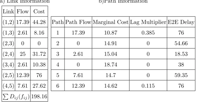
In the second step, the path flows for each session are calculated based on the optimal routing problem with end-to-end delay constraint, Problem 1. The end-to-end delay bound for each path is assumed to be 76 units in this simulation. The path flows are calculate by solving Problem1applying CVX package in MATLAB (see Table3).
The total cost of the network in step 2 is slightly higher than the optimum total cost in step 1. Yet in step 1 the individual path cost, for paths 1 and 6, is beyond the end-to-end delay bound. This means that this proposed algorithm is able to limit the delay with a minimum increase in the total cost. Also it can be seen that based on the Complementary Slackness condition,xp of paths 1 and 6 is decreased from the
optimum values of step 1, down to a point that their average delays are decreased to the threshold level. As such, the optimum dual variable, DV, of these two paths is expected to be higher than zero while DV of the other paths expected to be zero. It can be interpreted that the marginal cost of the paths 1 and 6 should be lower compared to that of path 3 for the calculated traffic.
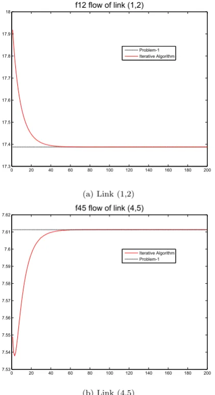
In the final step, the proposed algorithm is simu-lated through MATLAB. Here the step size is 0.008. The simulation finishes after 1000 iterations. The fi-nal results of the algorithm are presented in Table4. The stepwise results of the algorithm for Lagrange multipliers and two of the link flows as a sample are presented in Figure4and Figure5.
The results in Table4are the same as the results in Table3. This means that the iterative algorithm con-verges to the same results of the centralized solution. Figure 4 shows that the path flows converge to the same results as the results of the case where the Problem1is solved in a central manner.
Figure5shows that the Lagrangian multipliers of the distributed solution converge to the optimal dual variable values obtained from the centralized solution of the Problem1.
5
Conculsion
In this article a new method is introduced for traffic distribution in virtual circuit switched networks which can be implemented in real networks. In this method the input traffic of each session is distributed among the possible paths, in a manner that the total system cost is minimized at the same time as the average cost for each path is kept bounded below a required threshold level. This method is scalable as its operation is per session. It is analytically proven in this article that this algorithm converges under the assumptions that are feasible in real networks. The simulation results approve the effectiveness of the algorithm. The results obtained from the simulation are in line with the results obtained from analytical resolution of the convex optimization problem.
Appendix A
Mathematical Analysis
In this section the analysis of the proposed algorithm is provided. First some parameters used in this section are defined
• xp: Flow of the path p that is held in Assumption1
• H(X): Cost vector of all sessions withNP com-ponents where thepthcomponent represents the cost of thepthpath
Table 2. Simulation results of step1
a) Link Information b)Path Information Link Flow Cost
(1,2) 17.92 47.96 (1,3) 2.08 4.98
(2,3) 0 0
(2,4) 25.47 33.73 (3,4) 2.08 6.50 (2,5) 12.45 76.91 (4,5) 7.55 26.97
P
Dij(fij) 197.05
Path Path Flow Dual Varaible(DV) E2E Delay
1 17.92 11.55 81.68
2 0 13.55 54.46
3 2.08 11.55 11.48
4 0 16.74 33.48
5 7.55 14.74 60.7
6 12.45 14.744 76.91
Table 3. Simulation results of step 2
a) Link Information b)Path Information Link Flow Cost
(1,2) 17.39 44.28 (1,3) 2.61 8.16
(2,3) 0 0
(2,4) 25 31.72 (3,4) 2.61 10.38 (2,5) 12.39 76 (4,5) 7.61 27.62
PD
ij(fij) 198.16
Path Path Flow Marginal Cost Lag Multiplier E2E Delay
1 17.39 10.87 0.385 76
2 0 14.91 0 54.66
3 2.61 15.04 0 18.53
4 0 18.74 0 38
5 7.61 14.7 0 59.35
6 12.39 14.62 0.115 76
Table 4. Final results of Step3 for 1000 iterations and step size 0.008
a) Link Information b)Path Information Link Flow Cost
(1,2) 17.39 44.28 (1,3) 2.61 8.16
(2,3) 0 0
(2,4) 25 31.72 (3,4) 2.61 10.38 (2,5) 12.39 76 (4,5) 7.61 27.62
P
Dij(fij) 198.16
Path Path Flow Marginal Cost Lag Multiplier E2E Delay
1 17.39 10.87 0.385 76
2 0 14.91 0 54.66
3 2.61 15.04 0 18.53
4 0 18.74 0 38
5 7.61 14.7 0 59.35
0 20 40 60 80 100 120 140 160 180 200 17.3
17.4 17.5 17.6 17.7 17.8 17.9
18 f12 flow of link (1,2)
Problem-1 Iterative Algorithm
(a) Link (1,2)
0 20 40 60 80 100 120 140 160 180 200
7.53 7.54 7.55 7.56 7.57 7.58 7.59 7.6 7.61
7.62 f45 flow of link (4,5)
Iterative Algorithm Problem-1
(b) Link (4,5)
Figure 4. The flow of links per 200 iterations
0 20 40 60 80 100 120 140 160 180 200 0
0.05 0.1 0.15 0.2 0.25 0.3 0.35
0.4 Lagrangian Multiplier
L Multiplier P1 in It. Alg.
L Multiplier P5 in It. Alg.
L Multiplier P2-P5 in It. Alg. D. V. of P1 in Problem-1 D. V. of P6 in Problem-1
Figure 5. The Lagrangian multipliers corresponding to paths per 200 iterations
of thepthpath from its threshold
• T h: Threshold vector withNP components and thepthcomponent represents the maximum delay bound of the pathp
• Λ∗: Optimum solution of Problem4which is a vector withNP components
• λ∗p: Thepthcomponent of the optimum vector Λ∗, which is the optimum Lagrange multiplier of
thepthpath
Assumption 1. The value ofrw’s are such that
Prob-lem1has at least one strictly feasible point, in other words (16) is held.
∃X| X
p∈Pw
xp=rw & xp≥0 & hp(X)< thp
∀w∈W,∀p∈Pw (16) Result-1: Since the feasible set of the Problem1is not empty, this problem has at least one optimal point [19,20].
Proposition 1. The optimum solution of Problem4 is equal to the optimum solution of Problem2.
Proof. Since Problem 2 is a convex optimization problem, if the Slater conditions apply then the strong duality will also apply [19]. According to As-sumption 1 the Slater condition is held; therefore strong duality is held
Result-2: Assuming that the input traffic of sessions w meet (16), a strong duality exists and the optimum solution of Problem4is equal to the optimum solution of Problem2.
Result-3: Because of strong duality, (17) should hold for the optimum points of Problem2and Problem4
as follow:
λ∗p.(hp(x∗p)) = 0≡
(hp(x∗p)−thp<0⇒λ∗p= 0 (hp(x∗p)−thp= 0⇒λ∗p≥0
(17) According to (17), at the optimum point of Prob-lem4, the Lagrange Multiplier of the paths with lower costs than that of the threshold level is 0, and for the paths with Lagrange Multipliers greater than 0, the final traffic amount assigned to them will be such that the cost of these paths will be exactly equal to the threshold level.
Proposition 2. A) The function−q(Λ)defined in Problem4is a convex function ofΛ.
B) This function has subgradient at all of the points in its domain.
C,{{(x1...xn)|
X
p∈Pw
xp=rw, xp ≥0 ∀p∈Pw}}
Then
−q(Λ) =maximizeX∈C{−L(X,Λ)}
A)−qis a convex function: Defining vectorA(X) and functionb(X) by (18) and (19),−L(X,Λ) can be considered as a linear function of Λ for a given value of vectorX, as in (20)
A(X),T h−H(X) (18)
b(X),X p∈P
hp(xp) (19)
−L(X,Λ) =(A(X)T.Λ +b(X)) (20) Taking into account the definition given in (20) for functionL(X,Λ),−q(Λ) can be considered as the point-wise maximum of the family of linear functions at all points Λ according to (21); therefore−q(Λ) is a convex function [19].
−q(Λ)|Λ1 =maxX∈C{(A(X)T.Λ +b(X))|Λ1} (21)
B)Function−q(Λ) has subgradient at all points Λ: The −q(Λ) is differentiable at all points Λ where only oneX,X∗(Λ), maximizes (21), i.e. at these val-ues of Λ, only one of the functionsA(X)T.Λ +b(X)) is greater than the others; therefore at these points, the subgradient of the function is unique and is equal to its gradient which is calculated through (22).
∂−q(Λ)
∂Λ =∇(−q(Λ)) =A(X
∗(Λ)) =T h−H(X∗(Λ))
&
X∗(Λ) =arg(maxX∈C{(A(X)T.Λ +b(X))}) (22) The −q(Λ) is not differentiable at the points Λ where (21) is at its maximum at some points. At these Λ some of the functions (A(X)T.Λ +b(X)) have the greatest value at the same time. In this case, although
−q(Λ) is not differentiable, it has subgradient which is calculated through (23).
∂−q(Λ)
∂Λ |Λ1 =ConvexhullXi{(−A(X
∗
i(Λ)) T
}
&
X∗(Λ) =arg(maxX∈C{(A(X)T.Λ +b(X))}) (23)
λ = 0 K=0
End Criterion
= (ℎ ∗( ) − ℎ ) Solve Problem-3:
∗
= [ + . ]
End k=k+1
Figure 6.−q(λ) for one dimensionalλ
According to Proposition2, the functionq(Λ) is the point-wise infimum of a family of affine functions (21); hence, it is concave and sub-differentiable at any point (Figure6). In Proposition3an equation is provided to calculate one of the subgradient vectors of function
−q(Λ) that can be used in the algorithm in Figure2.
Proposition 3. At each pointΛb (24) gives the
sub-gradient of−q(Λ)at that point
Proof. According to (22,23) for a givenΛ, each opti-b
mal solution of (21),Xi∗,−A(Xi∗), is one of the sub-gradient vectors of −q(Λ) at pointΛ. According tob
(21), the optimal point of this equation at point Λb
can be obtained by solving Problem3based onΛ.b
−g(Λ) = (b T h−H(X∗))∈
∂q(Λ) ∂Λ |
b
Λ &
X∗(Λ) =arg(maxX∈C{(A(X)T.Λ +b(X))}) (24)
In other words,X∗(Λ) is an optimal point of
Prob-lem3based onΛ.b
Result-4: Considering (24) the number of compo-nents of vectorg(Λ) is equal to the total number ofb
threshold level. In this equation the path cost should be calculated when the traffic is the optimum solution of Problem3for vectorΛ. To calculate the subgradi-b
ent vector at pointΛ, solving Problemb 3at vectorΛb
and finding its optimum solutions suffices. Following this, the cost of each path is calculated for this traffic and its deviation from the threshold level is considered as the component of the subgradient vector.
Proposition 4. The algorithm introduced in Section3 converges:
Proof. As shown in Figure2, this algorithm describes the steps of the subgradient method in solving Prob-lem4. According to the proof given in [21], if the value of the subgradient of function−q(Λ) in all points has an upper bound such asGand if the distance from the initial point of the algorithm and the optimum point is less thanR, the subgradient method converges [21]. To prove the convergence of the algorithm, first, an upper bound for the distance of the initial point of this algorithm and the optimum point is introduced, and then the upper bound for the value of the sub-gradient vector of function −q(Λ) at all acceptable points is calculated.
A) Upper bound for the distance between the initial point Λ0and optimal point Λ∗:
The initial point of the proposed algorithm in this article is Λ0= 0. Assume a componentλ∗pis infinite. Considering Assumption-1 the amount of L(X,Λ∗) and alsog(Λ∗) is−∞. The optimal value of Problem3
will be−∞, while the optimal values of Problem 3
and Problem1were expected to be equal. considering Assumption-1 the optimal value of Problem1is finite (a contradiction); therefore all components of Λ∗ are finite, hence|Λ∗−Λ0|is bounded.
B) The norm of the subgradient vector in all itera-tions is upper bounded:
In iteration k, the component p of the subgradient vector is equal to the difference ofhp(X∗(Λk)) with
thp. Considering Assumption-1, (X∗(Λk) is a finite vector and since the optimal value of Problem1is fi-nite thenhp(X∗(Λk)) must be finite, hence, the norm of the vector is finite. Based on the maximum distance between the initial and the optimal points of the algo-rithm and the upper bound calculated for the subgra-dient at every step of the algorithm, the subgrasubgra-dient method for solving this problem will converge.
References
[1] Ning Wang, Kin-Hon Ho, George Pavlou, and Michael P. Howarth. An overview of routing optimization for internet traffic
engi-neering. IEEE Communications Surveys and Tutorials, 10(1-4):36–56, 2008. URL http:
//dblp.uni-trier.de/db/journals/comsur/ comsur10.html#WangHPH08.
[2] W.C.Hardy. Qos Measurement and Evaluation of Telecommunications Quality of Service. John Wiley & Sons, 2001.
[3] Xavier Masip-Bruin, Marcelo Yannuzzi, Jordi Domingo-Pascual, Alexandre Fonte, Mar´ılia Cu-rado, Edmundo Monteiro, Fernando A. Kuipers, Piet Van Mieghem, Stefano Avallone, Giorgio Ventre, Pedro A. Aranda-Guti´errez, Matthias Hollick, Ralf Steinmetz, Luigi Iannone, and Kav´e Salamatian. Research challenges in qos routing.
Computer Communications, 29(5):563–581, 2006. [4] Seung Yeob Nam, Sunggon Kim, and Dan Keun
Sung. Measurement-based admission control at edge routers. IEEE/ACM Trans. Netw., 16(2): 410–423, 2008. URLhttp://dblp.uni-trier. de/db/journals/ton/ton16.html#NamKS08. [5] Ishai Menache and Nahum Shimkin. Capacity
management and equilibrium for proportional qos. IEEE/ACM Trans. Netw., 16(5):1025–1037, 2008. URL http://dblp.uni-trier.de/db/ journals/ton/ton16.html#MenacheS08. [6] Mohamed E. M. Saad, Alberto Leon-Garcia, and
Wei Yu. Optimal network rate allocation un-der end-to-end quality-of-service requirements.
IEEE Transactions on Network and Service Man-agement, 4(3):40–49, 2007.
[7] Xavi Masip-Bruin, Marcelo Yannuzzi, Rene Serral-Gracia, Jordi Domingo-Pascual, Jose Enriquez-Gabeiras, Maria Angeles Callejo, Michel Diaz, Florin Racaru, Giovanni Stea, Enzo Mingozzi, Andrzej Beben, Wojciech Burakowski, Edmundo Monteiro, and Lus Cordeiro. The eu-qos system: a solution for eu-qos routing in heteroge-neous networks [quality of service based routing algorithms for heterogeneous networks]. Com-munications Magazine, IEEE, 45(2):96–103, Feb. 2007. ISSN 0163-6804. doi: 10.1109/MCOM. 2007.313402.
[8] Wojciech Burakowski, Andrzej Beben, Halina Tarasiuk, Jaroslaw Sliwinski, Robert Janowski, Jordi Mongay Batalla, and Piotr Krawiec. Provision of end-to-end qos in heterogeneous multi-domain networks. Annales des Tlcom-munications, 63(11-12):559–577, 2008. URL
http://dblp.uni-trier.de/db/journals/ adt/adt63.html#BurakowskiBTSJBK08. [9] Nan Jin and Scott Jordan. On the feasibility of
dynamic congestion-based pricing in differenti-ated services networks.IEEE/ACM Trans. Netw., 16(5):1001–1014, 2008.
re-sponsive yet stable traffic engineering. In Roch Gu´erin, Ramesh Govindan, and Greg Minshall, editors,SIGCOMM, pages 253–264. ACM, 2005. ISBN 1-59593-009-4.
[11] Neda Moghim, Seyed Mostafa Safavi, and Mas-soud Reza Hashemi. Performance evaluation of a new end-point admission control algorithm in ngn with improved network utilization.International Journal of Innovative Computing, Information and Control, 6(7), 2010.
[12] Leonard Kleinrock. Communication Nets; Stochastic Message Flow and Delay. McGraw-Hill Book Company, New York, 1964. (Out of Print.) Reprinted by Dover Publications, 1972 and in 2007. Published in Russian, 1971, Published in Japanese, 1975.
[13] R. Gallager. A Minimum Delay Routing Algo-rithm Using Distributed Computation. IEEE Transactions on Communications, 25(1):73–85, 1977. URL http://ieeexplore.ieee.org/ xpls/abs_all.jsp?arnumber=1093711. [14] D.P. Bertsekas, E. Gafni, R.G. Gallager,
Mas-sachusetts Institute of Technology. Labora-tory for Information, and Decision Systems. Sec-ond Derivative Algorithms for Minimum De-lay Distributed Routing in Networks. LIDS-P. Laboratory for Information and Decision Sys-tems, Massachusetts Institute of Technology, 1981. URLhttp://books.google.com/books? id=V5zpHAAACAAJ.
[15] Dimitri P. Bertsekas and Robert G. Gallager.
Data Networks, Second Edition. Prentice Hall, 1992. ISBN 978-0-13-201674-2.
[16] Christos G. Cassandras, M. Vasmi Abidi, and Don Towsley. Distributed routing with on-line marginal delay estimation. IEEE Transactions on Communications, 38(3):348–359, 1990. [17] A. Segall. The modeling of adaptive routing in
data-communication networks.Communications, IEEE Transactions on, 25(1):85 – 95, jan 1977. ISSN 0090-6778.
[18] A. Segall, M. Sidi, Massachusetts Institute of Technology. Laboratory for Information, and Decision Systems. A Failsafe Distributed Pro-tocol for Minimum Delay Routing. LIDS-P. Laboratory for Information and Decision Sys-tems, Massachusetts Institute of Technology, 1981. URLhttp://books.google.com/books? id=2YOxtgAACAAJ.
[19] S. P. Boyd and L. Vandenberghe. Convex Opti-mization. Cambridge University Press, 2004. [20] D. P. Bertsekas.Nonlinear programming. Athena
Scientific, 1999.
[21] S. Boyd, L. Xiao, and A. Mutapcic. Subgradient methods, 2003.
Touraj Shabanianreceived the B.Sc. and M.Sc. in electrical engineering from the Isfa-han University of Technology, IsfaIsfa-han, Iran, in 2001, 2005, and Ph.D. degrees in electri-cal engineering from the Isfahan University of Technology, Isfahan, Iran, in 2013. His re-search interests include QoS and traffic man-agement in large-scale networking systems, network optimization and graph theory with emphasis on routing algorithms.
Massoud Reza Hashemireceived his BSc and MSc from Isfahan University of Technol-ogy in 1986 and 1988 respectively, and his PhD from the University of Toronto in 1998, all in Electrical and Computer Engineering. From 1988 to 1993 he was with Isfahan Uni-versity of Technology as a faculty member. From 1998 to 1999 he was a postdoctoral fel-low at the University of Toronto. From 1999 to 2002 he was a founding member and lead systems architect of AcceLight Networks, where he developed some of the key system elements of a multi-terabit multiservice core switch. Since 2003 he has been with Isfahan University of Technology. His current research interests include Software Defined Net-works, Data Centric NetNet-works, DSM in Smart Grid, and Alert Correlation in Network Intrusion Detection.
Ahmad Askarianreceived the Bachelor de-gree in electrical engineering from the Shahed University, Tehran, Iran, in 2008 and the M.E. degree from the Isfahan University of Tech-nology (IUT), Isfahan, Iran, in 2010. He is currently pursuing the doctoral degree at the University of Texas at Dallas (UTD). Since 2012, he is a research assistant in the Scalable Network Engineering Techniques Laboratory, UTD, Dallas, US. His research interests include network optimization and graph theory with emphasis on routing algorithm.