Methodology
Case-crossover and case-time-control studies: concepts, design, and analysis
Seyed Saeed Hashemi Nazari1, Mohammad Ali Mansournia2*
1 Safety Promotion and Injury Prevention Research Center AND Department of Epidemiology, School of Public Health, Shahid
Beheshti University of Medical Sciences, Tehran, Iran
2 Department of Epidemiology and Biostatistics, School of Public Health, Tehran University of Medical Sciences, Tehran, Iran
ARTICLE INFO ABSTRACT
Received 07.04.2014 Revised 21.07.2014 Accepted 07.09.2014 Published 20.2.2015
Available online at: http://jbe.tums.ac.ir
Background & Aim: Case-crossover studies are the case-control version of crossover studies. In
these studies, cases and controls are the same subjects. The term crossover is applied for designs that all subjects pass through both treatment (exposure) and placebo (non-exposure) phases. In fact they are crossover of subjects between periods of exposure and non-exposure. This design is most suitable for outcomes, which their induction time is short. Whatever the onset of outcome is more abrupt, it is more amenable to be studied in case-crossover studies. Case-crossover design can be implemented in a number of ways. In this article some common terms in the literature of case- crossover studies, major concerns in selection of controls, different ways for designing case-crossover studies, some examples for analyzing these data according to different sampling designs and also design and analysis of case-time-control designs with practical examples are being explored.
Key words: case-crossover, case-time-control, design and analysis
Introduction1
Case-crossover studies are the case-control version of crossover studies. In these studies, cases and controls are the same subjects, but in two (one case to one control) or more than two (one case to more than one control) different times. This concept was introduced by Maclure et al. in their attempt to avoid control selection bias to test hypotheses concerning the immediate determinants of myocardial infarction (MI) (1, 2). Since then, this design has been used for studying the effect of exposures such as physical activity, anger, sexual activity, cocaine use, bereavement, exertion, and respiratory infections on MI, the effect of car telephone calls on risk of collision, the effect of air pollution on daily mortality and etc. (3, 4). The characteristic
* Corresponding Author: Mohammad Ali Mansournia, Postal
Address: Department of Epidemiology and Biostatistics, School of Public Health, Tehran University of Medical Sciences, P.O. Box 14155-6446, Tehran, Iran. Email: [email protected]
feature of this design is that each case serves as its own control in other times. This design is somehow similar to crossover study if we look at it in a retrospective way except that exposure assignment is not at the control of the investigator.
The term crossover is applied for designs that all subjects pass through both treatment (exposure) and placebo (non-exposure) phases. In case-crossover design, the terms denotes crossover of subjects between periods of exposure and non-exposure (1). In spite of its similarities to retrospective cohort studies, in this design exposure frequency is measured in just a sample of the total time at risk. Thus, a case-crossover study resembles a nested case control study and odds ratio (OR), which is estimated in this design is interpreted as rate ratio.
Case-crossover design can be implemented in a number of ways. In its simplest design, every case has one control, which is the same subject at a different time period. Since cases and controls are matched according to all
characteristics except time dependent variables, this specific design is like a pair-matched case control design.
Suppose a researcher want to assess the relation between bottle feeding and sudden infant death with simple case-crossover design. In this example, cases are infants with diagnosis of sudden cardiac death and controls are the same infants in another time period, for example, in the previous day of death at the same clock-hour of death. The exposure in this example is bottle feeding during the preceding hour, which is evaluated once for cases during the previous hour of death and once for controls during the preceding hour of the same clock-time in the previous day of death. In this example, if an infant dies at 8 p.m. on 20th of October, his/her status at 8 p.m. on the 19th of October is considered as control and his/her bottle feeding in the preceding hour from 7 to 8 p.m. is considered as his/her exposure status in both case and control status.
This design is most suitable for outcomes, which their induction time (5) is short. Whatever the onset of outcome is more abrupt, it is more amenable to be studied in case-crossover studies. Thus, an ischemic heart attack which has an abrupt onset can be studied for the exposures which may have triggered it or a car accident which can be timed accurately can be studied for the triggers which had happened just minutes before it (2).
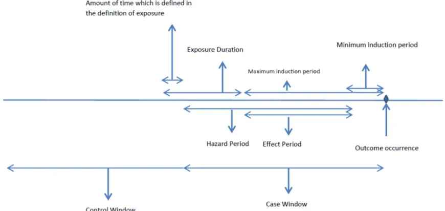
The definition of some common terms in case-crossover design makes extracting necessary data for analyzing theses designs more feasible. Induction time (period) is the time between a component cause and its effect. For example, for the effect of smoking on lung cancer induction time is the time between beginning smoking and onset of cancer and in the study of the effect of mobile phone call on car accident, the induction time is the time between the phone call and car accident. Exposure, which have short induction time are more feasible to be assessed in case-crossover studies, although, exposure with long induction time (6) can also be assessed with this design.
Effect period is the time between the minimum induction time and maximum
induction time for the effect of a specific exposure on an outcome in the population under study. Sometimes, the minimum induction period is zero; in these situations, effect period is equal to maximum induction period. For example, in the study of the association between cellular-telephone calls and motor vehicle collision the minimum induction period was zero and the maximum induction period was considered 5- 15 min (7). Maximum induction time includes the time denoted as washout period in crossover experiments, after which carryover effect are hypothesized not to occur. According to this definition, washing period is included in the effect period and then an exposure outside this period is unlikely to be a cause of an outcome. Exposures are suitable for case-crossover studies, which either do not have a carry-over effect or it lasts a short time (2). The best estimate of effect period is the one that maximized the effect measure.
Hazard period is the time interval after an exposure when an individual experiences an increased risk of the outcome. This period equals duration of exposure plus the effect period minus the amount of time, which is specified in the definition of exposure. If exposure happens fast, hazard period equals effect period, but if exposure is not instantaneous, hazard period is longer than effect period. The risk of outcome is not the same during hazard period, and this period can be divided into several smaller hazard periods with different degrees of risk (1).
exercise remains in the 90 min duration after the first 10 min of exercise, but if he/she gets MI after 101 min after the beginning of exercise, with the above mentioned criteria he is not considered as an exposed case. In this example, if a person exercise for 5 min and then gets MI, he is not considered exposed case because in this example we are studying the effect of 10 min exertion or higher on the risk of MI.
Estimation of effect period is usually imprecise because of both variations in induction times and also uncertainty about the time of exposure and occurrence of outcome.
For each case, the period of time that the exposure under study can potentially have an effect on the current outcome is named case window. Case window equals the hazard period before the occurrence of outcome. Exposure assessment is performed during this window. The time before case window is considered as control window. Control selection and exposure assessment for control is performed in this window. Sometimes, this control window can contains the time after case window. Figure 1 illustrates these definitions in a case-crossover study.
Control times are selected from the control window. If the frequency of exposure under study does not change after the occurrence of
outcome, it is also possible to consider the time after the occurrence of outcome as control window and to select some controls from this window.
There are some issues to be considered when we are selecting the control times from control window. The first one is whether we should exclude the sleep times or the times where the exposure is impossible to happen?
Various studies of triggers of MI have acted differently on inclusion or exclusion of sleep times. Willich et al. excluded sleep times (8), but some other researchers have included them (9-11).
In the study of the relation of exertion and MI people are at danger of MI even in sleep time. In this situation if researcher includes the MIs, which have occurred at the sleep time and excludes these times from the control window, the study suffers from selection bias. As long as the same restriction applies to case times and control times, selection bias will be avoided. In another word, if one include the outcomes which have occurred at the sleep times, it is not suggested to exclude these times from control window even if the occurrence of the exposure under study is impossible at those times. If an outcome is unlikely to happen in the sleeping time, we can restrict the study to the walking time (12).
Figure 1. Illustration of some common terms in the case-crossovver studies
Another issue worth mentioning is that control window is not always before case window. If the outcome under study does not affect the occurrence of exposure, the time after outcome occurrence can also be considered as control window, and both past and future control times can be used. Such bidirectional sampling has been used in air pollution studies because people’s outcome do not affect the amount of air pollution level, unless their outcome affect their chance of being exposed by forcing them to stay at home or leave the town (13). In the absence of changes in exposure frequency, control windows may be sampled outside the period during which the subjects would be considered at risk for the outcome.
The third issue to be discussed is choosing control windows from periods that person is not at risk of the outcome. In these situations also the assumption of independence of exposure and the context of being at risk for the outcome is necessary. For example, suppose a researcher want to assess the relation of cell phone call and car accident in a case-crossover study. Cases are subjects who have accident. In these subjects exposure of interest which is talking with a cell phone in 10 min before accident occurrence is evaluated. Controls are these people at the same clock-time on the day before the accident on the condition that at that time, they were also driving. This condition can be relaxed when the researcher assumes that mobile cell phone call in not associated with driving. Driving in this example is the context that makes people at danger of outcome under study. Without such assumption choosing control from the control window that subjects are not in danger of outcome results in a biased estimate.
Design and Analysis of Case-Crossover Studies
There are a number of ways for designing a case-crossover study. In the common approach which is similar to one to one pair match case control studies, exposure in the hazard period before the outcome is compared with exposure in the comparable control period at the same time of the day in some day before the occurrence of outcome (1, 14). In this approach
because the case and controls time are adjusted for the clock time in a matched analysis, nothing is assumed about the effect of clock-time and baseline hazard is let to vary with clock time in a way that is unique for each individual.
In another strategy instead of one control period, more than one control periods are sampled from the control window per case and exposure of the case in the hazard period is compared with exposure assessment in these control windows. This design is similar to an M-to-one matched case control design.
In this approach researcher sample, more than one control period matched or unmatched to the clock time of outcome occurrence The advantage of this approach is that if one assumes that clock times in a day is a confounder or effect modifier of the effect of interest, by choosing control period from different clock times in a day (unmatched strategy), the effect of clock time can be measured and controlled (15).
In the third approach which is sometimes called “ usual frequency method,” exposure in the hazard period is compared with the expected frequency of exposure, based on each subject usual frequency of exposure over a specific control period, before the outcome. In this approach researcher assumes no confounding by clock time.
The efficiency of relative risk estimators in case-crossover studies varies according to the sampling strategies. Comparison of these sampling approaches in a study of association of exertion and MI showed that, the variance of relative risk was decreased with an increase in the number of controls per cases, and the efficiency of the usual frequency approach was highest (15). There are large trade-offs between efficiency and potential bias inherent in the choice of control sampling procedure (15).
The recommended methods for analysis of case-crossover studies are conditional logistic regression, and Mantel-Haenszel incidence rate ratio estimator with confidence intervals for sparse data (2, 16).
Some examples of analysis of case-crossover designs with above mentioned sampling approaches are as follows.
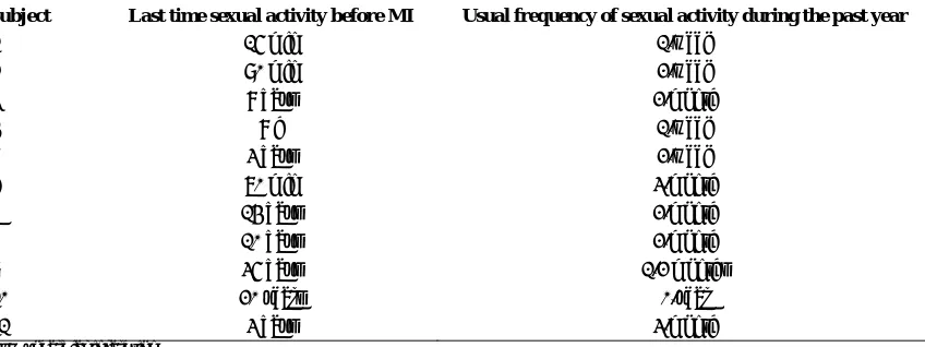
First example
subjects from a hypothetical case-crossover study on the association of MI and sexual activity. Subjects were asked when the last time of sexual activity before their MI was and also what the usual frequency of their sexual activity during the past year was. The hazard period once was considered equal to 1 h and once was considered equal to 2 h.
The structure of dataset for analyzing case-crossover data gathered by usual frequency method for the first two subjects of table 1 has been shown in appendix. The Mantel-Haenszel estimate of the rate ratio (95% confidence interval) is 21.2 (2.6 - 169.9). In Stata software (all versions), ir command performs this analysis. The conditional maximum likelihood estimate of rate ratio (95% confidence interval) is 21.9 (2.6 -181.1). In Stata, clogit command with the natural logarithm of time as offset performs this analysis.
In the above example, the duration of hazard period was considered 1 h. The actual duration of the effect period can be determined empirically by examining the change in the rate ratio under different magnitudes of hazard period. In the above example, if we consider hazard period as 2 h the data for the first two subjects will be similar to the second part of table A1 in appendix. In this situation, relative rate will be 46.37 with a confidence interval of 11.2 - 192.1.
The usual frequency method is very sensitive to the calculation of probability of being exposed and being unexposed. In this example, the probability of being exposed was calculated
by multiplying the rate of exposure (ƛ: number of exposure per hour ) by hazard period (1 h). For example, for the second person, the probability of being exposed was ƛ * t = (104/8766) * 1. Assuming a Poisson model for occurrence of sexual activity, for small “ƛt” (rate * hazard periods), say <0.1, this way of calculating the probability as an estimate of the true probability is approximately true, but if “ƛt”
is not small, the probability should be calculated by 1 − exp(−ƛt). For example, in the above example if hazard period was long (e.g., 24 h), the probability of at least one sexual activity in the hazard period should be estimated by 1 −
exp(−24 * rate of sexual activity per hour) (11).
Second example
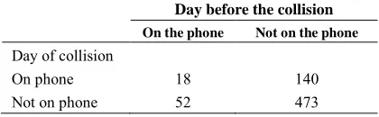
Table 2 shows a portion of hypothetical data on the association between cellular-telephone calls and motor vehicle collisions (7). In this hypothetical study, 683 drivers who owned a cell phone and had collision were studied. Hazard period was considered 15 min before the estimated time of the collision. The control time is the same clock time on the day before collision. Method of sampling is pair matched sampling. The structure of data for analyzing this study is shown in table A5 in appendix.
The data in table 2 can be analyzed with fitting a conditional logistic model ( clogit command in Stata). The maximum likelihood estimate of OR is 2.6 (1.9- 3.7).
Table 1. Data of a hypothetical case-crossover study of the effect sexual activity on Ml
Subject Last time sexual activity before MI Usual frequency of sexual activity during the past year
1 15 min 1/week
2 90 min 2/week
3 8 days 2/month
4 8 h 1/week
5 3 days 2/week
6 70 min 3/month
7 14 days 2/month
8 10 days 2/month
9 35 days 1/2 months
10 20 years 0/year
11 3 days 3/month
MI: Myocardial infarction
Table 2. Data of a hypothetical case-crossover study on
association of cellular telephone use and car collision Day before the collision
On the phone Not on the phone Day of collision
On phone 18 140
Not on phone 52 473
Case-time-control design
When there is a time trend in distribution of exposure in the population under study, case-crossover design estimate of the rate ratio is biased. Case-time-control design developed to remove this probable bias in case-crossover design. In this design, cases and controls are selected similar to a case control design, and then for each groups of cases and controls a case-crossover study is designed. In another word, cases are assessed for exposure twice, once in case window and once in the control window (similar to a case-crossover design performed on cases). Controls are also assessed twice for occurrence of exposure, once in the hypothesized case window and once in the control window (again similar to a case-crossover design which is performed this time on controls). In this design, among the controls matched OR comparing odds of exposure in the hypothesized case window to odds of exposure in the control window measures the time trend in exposure. Among the cases matched OR comparing odds of exposure in the case window to odds of exposure in the control window measures the time trend in exposure and also the effect of exposure. The case-time-control OR is equal to OR among the cases divided by OR among the controls (17).
In case-time-control design researcher can fit two models on two groups of data, once for the control group (model 1) and once for case group (model 2):
Model 1: Logit Period = β0 + β1 Exposure
Model 2: Logit Period = θ0 + θ1 Exposure
Where “Exposure” denotes to exposure situation (1 = exposed, 0 = non-exposed),
Period” denotes to period (1 = current case
window for both case and control group, 0 = reference control window for both case and control group) and Group denotes to group status (1 = case, 0 = control).
In model 1, which is fitted on the control group, exp(β1) is the OR of period effect (odds
of being exposed in period 1 hypothesized case window versus odds of being exposed in period 0 hypothesized control window). Since no one in this group is case, exp(β1)
shows just trend of exposure.
In model 2, which is fitted on case group,
exp(θ1) is the OR of period effect plus exposure
effect. If we assume that the case-crossover OR is the product of OR due to effect of exposure on the outcome and OR due to time trend in exposure prevalence and also the time trend of exposure is the same in two groups (case group and control group) then the case-crossover OR can be estimated by dividing exp(θ1) by
exp(β1).
By this method of analysis point estimate of OR for effect of exposure on the outcome controlled for period effect can be estimated but what about its confidence interval? The above two models can be summed up in one model (model 3):
Model 3: Logit Period = a0+ a1 Exposure + a2 Exposure * Group
In this model, exp(a1) is the effect of exposure change on odds of case period versus control period in the control group (since control group subjects are all outcome negative and exposure has compared in two different times, exp(a1) is the time trend effect of exposure an equals to exp(β1) in model 1.
Exp(a2) in this model is the effect of exposure change adjusted for effect of exposure time trend on odds of case period versus control period. It is the measure of interest in this design since it is interpreted as odd ratio of getting the outcome in exposed versus unexposed adjusted for time trend effect of exposure. Exponential of (a1 + a2) is the measure which is estimated in the usual case-crossover design which is the combination of exposure effect and time trend effect of exposure (it is equal to exp(θ1) in
model 2) (18, 19).
Example 3
one or more congenital anomalies were chosen as cases. Mothers were considered as exposed if they reported having used vitamin x any time during the first trimester after the last menstrual period. Three months before the last menstrual period were considered as control window (with the assumption that pregnancy does not change the prevalence of using vitamin x). Controls were a random sample of women who did not have infant with birth defect. These controls were also assessed for exposure occurrence in their case window and control window exactly the same as case group (Table 3).
Constructing a dataset according to the example 2 and fitting a conditional logistic model on the cases as a separate case crossover study gives the OR of 0.55 (0.33 - 0.91) and on controls gives the OR of 0.51 (0.34 - 0.77). As it was mentioned above, the first OR presents the effect of exposure under study and also time trend in exposure on the outcome and the second OR presents the effect of time trend of exposure. If we divide the first OR by the second, the pure effect of exposure will be OR = 1.06.
This OR and its confidence interval can be estimated with fitting model 3 on the data with exposure and interaction of exposure and group as independent variables. The structure of these data is presented in appendix in table A3.
Fitting conditional logistic regression on this data, the estimate of a1 will be −0.66 and the
estimate of a2 will be 0.062.
The OR of exposure controlled for period effect is 1.0 (0.5 - 2.3) which in this hypothetical dataset, vitamin x did not have a statistically significant effect on the congenital defect and almost all the observed effect was because of time trend in exposure.
Discussion
In a case-crossover study, only cases with discordant exposure status in the case and control window contribute to the effect measure estimation. Therefore, an application of this design is for time-varying or intermittent exposures. Because in this design, cases and controls are the same person, the problem of between-person confounding by constant characteristics do not occur (20). However, the problem of within person confounding still can occur. This problem can occur when multiple of transient exposures are correlated in time within an individual. For example, in the analysis of association of sexual activity and MI it is possible that the association is confounded by episodes of anger. If data regarding assessment of confounders in both case and control windows are collected, by sampling strategies one and two, researcher can adjust for such confounders using conditional logistic regression with terms entered in the model for confounders. In the third sampling strategy, usual frequency approach, controlling for confounder is a bit difficult. In this approach for controlling confounders, it is necessary to collect information on the usual frequency of exposure conditional to other potential within person confounders. For example, if anger episodes are confounders, the following question should be asked from subjects: how often during the past year have you been angry during the sexual activity? This question and similar question to this one are difficult to answer let alone the researcher wants to collect the usual frequency of another confounder either. Therefore, the inability to control for within person confounding is a limitation of usual frequency approach (15).
Table 3. Data of hypothetical case-time-control design showing the risk of congenital defects due to exposure
to vitamin x during the first trimester of pregnancy
Case window (period 1)
Cases (infants with a congenital defect) Controls
Exposed Non-exposed Exposed Non-exposed Control window (period 0)
Exposed 56 23 84 36
Non-exposed 42 3400 70 7700
Total 98 3423 154 7736
The choice of sampling strategy depends on the tradeoff between precision and bias. The usual frequency approach usually produces the most efficient estimators but within person confounders are hard to control in this approach. Therefore, in studies which within person confounders are negligible, this is a good sampling strategy.
When the frequency of exposure changes over time, case-crossover study might produce bias estimates. In a rare situation that outcome under study does not affect the future exposure, it is possible to use future periods as control times. This approach reduces the problem of exposure time trend bias (20). Another approach for dealing with this problem is case-time-control design. Bias due to time trends in exposure can be removed by case-time-control design, but if an uncontrolled time-varying confounder such as disease severity (confounding by indication) is present, the use of crossover in controls can introduce new confounding (21). The necessary assumption for this approach to be valid is that variation in frequency of exposure in time depends not on some unmeasured characteristics in individuals. In another word, there should not be any interaction between unmeasured confounders and period on exposure.
References
1. Maclure M. The case-crossover design: a method for studying transient effects on the risk of acute events. Am J Epidemiol 1991; 133(2): 144-53.
2. Maclure M, Mittleman MA. Should we use a case-crossover design? Annu Rev Public Health 2000; 21: 193-221.
3. Maclure M, Mittleman MA. Cautions about car telephones and collisions. N Engl J Med 1997; 336(7): 501-2.
4. Mittleman MA, Maclure M, Sherwood JB, Mulry RP, Tofler GH, Jacobs SC, et al. Triggering of acute myocardial infarction onset by episodes of anger. Determinants of Myocardial Infarction Onset Study Investigators. Circulation 1995; 92(7): 1720-5. 5. Rothman KJ, Greenland S, Lash TL. Modern Epidemiology. Philadelphia, PA: Lippincott
Williams & Wilkins; 2008.
6. Dixon KE. A comparison of case-crossover and case-control designs in a study of risk factors for hemorrhagic fever with renal syndrome. Epidemiology 1997; 8(3): 243-6. 7. Redelmeier DA, Tibshirani RJ. Association
between cellular-telephone calls and motor vehicle collisions. N Engl J Med 1997; 336(7): 453-8.
8. Willich SN, Lewis M, Lowel H, Arntz HR, Schubert F, Schroder R. Physical exertion as a trigger of acute myocardial infarction. Triggers and Mechanisms of Myocardial Infarction Study Group. N Engl J Med 1993; 329(23): 1684-90.
9. Gullette EC, Blumenthal JA, Babyak M, Jiang W, Waugh RA, Frid DJ, et al. Effects of mental stress on myocardial ischemia during daily life. JAMA 1997; 277(19): 1521-6.
10. Hallqvist J, Moller J, Ahlbom A, Diderichsen F, Reuterwall C, de Faire U. Does heavy physical exertion trigger myocardial infarction? A case-crossover analysis nested in a population-based case-referent study. Am J Epidemiol 2000; 151(5): 459-67.
11. Marshall RJ, Jackson RT. Analysis of case-crossover designs. Stat Med 1993; 12(24): 2333-41.
12. Petridou E, Mittleman MA, Trohanis D, Dessypris N, Karpathios T, Trichopoulos D. Transient exposures and the risk of childhood injury: a case-crossover study in Greece. Epidemiology 1998; 9(6): 622-5. 13. Navidi W. Bidirectional case-crossover
designs for exposures with time trends. Biometrics 1998; 54(2): 596-605.
14. Breslow NE, Day NE. Statistical methods in cancer research: Vol. 1: The analysis of case-control studies. Lyon, France: International Agency for Research on Cancer; 1980.
15. Mittleman MA, Maclure M, Robins JM. Control sampling strategies for case-crossover studies: an assessment of relative efficiency. Am J Epidemiol 1995; 142(1): 91-8.
follow-up data. Biometrics 1985; 41(1): 55-68. 17. Hernandez-Diaz S, Hernan MA, Meyer K,
Werler MM, Mitchell AA. Case-crossover and case-time-control designs in birth defects epidemiology. Am J Epidemiol 2003; 158(4): 385-91.
18. Suissa S. The case-time-control design. Epidemiology 1995; 6(3): 248-53.
19. Suissa S. The case-time-control design: further assumptions and conditions.
Epidemiology 1998; 9(4): 441-5.
20. Schneeweiss S, Sturmer T, Maclure M. Case-crossover and case-time-control designs as alternatives in pharmacoepidemiologic research. Pharmacoepidemiol Drug Saf 1997; 6(Suppl 3): S51-S59.
21. Greenland S. Confounding and exposure trends in case-crossover and case-time-control designs. Epidemiology 1996; 7(3): 231-9.
Appendix
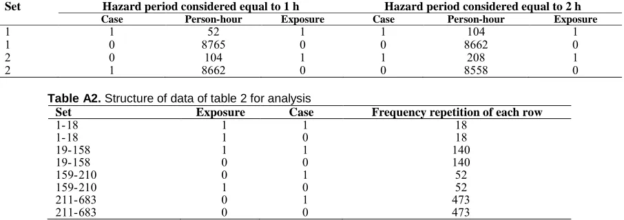
Table A1 shows the structure of dataset for analyzing case-crossover data gathered by usual frequency method for the first two subjects of table 1. Each subject has two records in the dataset one as case and one as control. The first subject had one sexual activity every week during the past year. Hence, during the past year he had 52 person-hours exposed time and 8714 person-hours unexposed time. In another word, the probability of being exposed was 52/8766 and the probability of being unexposed was 8714/8766 for this person. Because this person got MI in <1 h after sexual activity, he got MI in the exposed time. The second subject had two sexual activities per week during the past year. Hence, during the past year he had 104 person-hours exposed time and 8662 person-person-hours unexposed time. Because this person got MI in more than 1 h (1 h is hazard period) after sexual activity, he got MI in the unexposed time.
Table A2 shows the structure of dataset for analyzing hypothetical study represented in table 2. The first row of this table shows an exposed person in the case window. The second row shows the same person in the control window and in this time he is also exposed. According to table 2, there should be 18 sets of person similar to the first and second row of this table in the dataset. Similarly, the 7th row of this table shows a non-exposed person in the case window and the 8th row shows the same person in the control window and in this time he/she is non-exposed.
According to table 2 there should be 473 sets of person similar to the 7th and 8th row of this table in the dataset. Totally, the dataset for analyzing these data should have 683 sets of individuals and 1366 rows of data.
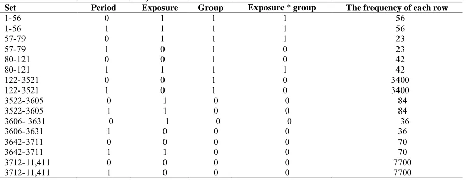
The structure of dataset for analyzing table 3 data is presented in table A3. This table consists of four variables. Group variable defines whether subject belonged to case group (group = 1) or control group (group = 0). Period defines whether the data of this record belongs to the case window (current period, period = 1) or control window (reference period, period = 0), exposure defines whether the subject was exposed during that period (exposure = 1) or not exposed (exposure = 0) and group exposure variable defines the interaction of group variable and exposure variable. The first row of this table shows an exposed person in the case group in the case window. The second row shows the same person in the control window and in this time he is also exposed. According to table 3, there should be 56 sets of persons similar to the first and second row of this table in the dataset. Similarly, the 11th row of this table shows an exposed person in the control group in the case window. And, the 12th row shows the same person in the control window and in this time he is non-exposed. According to table 3, there should be 36 sets of person similar to the 11th and 12th row of this table in the dataset. Totally, the dataset for analyzing these data should have 11,411 sets of individuals and 22,822 rows of data.
Table A1. Structure of data for the first two subject of table 1 once for hazard period equal to 1 h and once for hazard
period equal to 2 h
Set Hazard period considered equal to 1 h Hazard period considered equal to 2 h
Case Person-hour Exposure Case Person-hour Exposure
1 1 52 1 1 104 1
1 0 8765 0 0 8662 0
2 0 104 1 1 208 1
2 1 8662 0 0 8558 0
Table A2. Structure of data of table 2 for analysis
Set Exposure Case Frequency repetition of each row
1- 18 1 1 18
1- 18 1 0 18
19- 158 1 1 140
19- 158 0 0 140
159- 210 0 1 52
159- 210 1 0 52
211- 683 0 1 473
Table A3. The data structure for analysis of table 3
Set Period Exposure Group Exposure * group The frequency of each row
1- 56 0 1 1 1 56
1- 56 1 1 1 1 56
57- 79 0 1 1 1 23
57- 79 1 0 1 0 23
80- 121 0 0 1 0 42
80- 121 1 1 1 1 42
122- 3521 0 0 1 0 3400
122- 3521 1 0 1 0 3400
3522- 3605 0 1 0 0 84
3522- 3605 1 1 0 0 84
3606- 3631 0 1 0 0 36
3606- 3631 1 0 0 0 36
3642- 3711 0 0 0 0 70
3642- 3711 1 1 0 0 70
3712- 11,411 0 0 0 0 7700
3712- 11,411 1 0 0 0 7700