Gabriel Caloz & Monique Dauge, Editors
MODIFIED DIFFERENTIAL EQUATIONS
∗Philippe Chartier
1, Ernst Hairer
2and Gilles Vilmart
1,2Dedicated to Prof. Michel Crouzeix
Abstract. Motivated by the theory of modified differential equations (backward error analysis) an approach for the construction of high order numerical integrators that preserve geometric properties of the exact flow is developed. This summarises a talk presented in honour of Michel Crouzeix.
R´esum´e. Motiv´e par la th´eorie des ´equations modifi´ees (analyse r´etrograde de l’erreur), une approche pour la construction de m´ethodes num´eriques d’ordre ´elev´e pr´eservant des propri´et´es g´eom´etriques du flot exact est d´evelopp´ee. Ceci r´esume une pr´esentation donn´ee en honneur de Michel Crouzeix.
Introduction
Modified differential equations in combination with backward error analysis (cf. the monographs [3], [5]) form an important tool for studying the long-time behaviour of numerical integrators for ordinary differential equations. The main idea of this theory is sketched and, by inverting the roles of the exact and numerical flows, a new approach for the construction of high order numerical integrators for ordinary differential equations is developed [1]. As an application, a computationally efficient and highly accurate modification of the Discrete Moser–Veselov algorithm for the simulation of the free rigid body is presented [4].
1.
Modified equations for backward error analysis
Consider an initial value problem
˙
y=f(y), y(0) =y0 (1)
with sufficiently smooth vector field f(y), and a numerical one-step integrator yn+1 = Φf,h(yn). The idea of
backward error analysis is to search for a modified differential equation
˙
z=fh(z) =f(z) +hf2(z) +h2f3(z) +. . . , z(0) =y0, (2)
which is a formal series in powers of the step sizeh, such that the numerical solution{yn}is formally equal to the exact solution of (2),
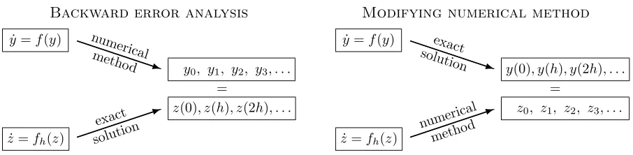
yn=z(nh) for n= 0,1,2, . . . , (3) see the left picture of Figure 1.
∗This work was partially supported by the Fonds National Suisse, project No. 200020-109158.
1 INRIA Rennes, Campus de Beaulieu, 35042 Rennes-Cedex, France
2 Section de Math´ematiques, Universit´e de Gen`eve, 2–4 rue du Li`evre, CH-1211 Gen`eve 4, Switzerland c
EDP Sciences, SMAI 2007
q
1
Backward error analysis
˙ y=f(y)
˙
z=fh(z)
z(0), z(h), z(2h), . . . =
y0, y1, y2, y3, . . . numerical
method
exact solution
q
1
Modifying numerical method
˙ y=f(y)
˙
z=fh(z)
y(0), y(h), y(2h), . . . =
z0, z1, z2, z3, . . . exact
solution
numerica l
method
Figure 1. Backward error analysis opposed to modifying numerical integrators
The idea of backward error analysis was originally introduced by Wilkinson (1960) in the context of numerical linear algebra. For the integration of ordinary differential equations it was not used until one became interested in the long-time behaviour of numerical solutions. Without considering it as a theory, Ruth [9] uses the idea of backward error analysis to motivate symplectic integrators for Hamiltonian systems. In fact, applying a symplectic numerical method to a Hamiltonian system ˙y = J−1∇H(y) gives rise to a modified differential
equation that is Hamiltonian. This permits to transfer known properties of perturbed Hamiltonian systems (e.g., conservation of energy, KAM theory for integrable systems) to properties of symplectic numerical integrators. One became soon aware that this kind of reasoning is not restricted to Hamiltonian systems, and new insight can be obtained with the same techniques also for reversible differential equations, for Poisson systems, for divergence-free problems, etc. A rigourous analysis has been developed in the nineties. We refer the interested reader to [3, Chapter IX], where backward error analysis and its applications are explained in detail.
2.
Modifying numerical integrators
Backward error analysis is a purely theoretical tool that gives much insight into the long-term integration with geometric numerical methods. We shall show that by simply exchanging the roles of the “numerical method” and the “exact solution” (cf. the two pictures in Figure 1), it can be turned into a means for constructing high order integrators that conserve geometric properties. They will be useful for integrations over long times.
Let us be more precise. As before, we consider an initial value problem (1) and a numerical integrator. But now we search for a modified differential equation, again of the form (2), such that the numerical solution {zn}of the method applied with step sizehto (2) yields formally the exact solution of the original differential equation (1), i.e.,
zn=y(nh) for n= 0,1,2, . . . , (4) see the right picture of Figure 1. Notice that this modified equation is different from the one considered before. However, due to the close connection with backward error analysis, all theoretical and practical results have their analogue in this new context. The modified differential equation is again an asymptotic series that usually diverges, and its truncation inherits geometric properties of the exact flow if a suitable integrator is applied. The coefficient functions fj(z) can be computed recursively by using a formula manipulation program likemaple. This can be done by developing both sides ofz(t+h) = Φfh,h(z(t)) into a series in powers ofh, and by comparing their coefficients. Once a few functionsfj(z) are known, the following algorithm suggests itself.
Algorithm 2.1 (modifying integrator). Consider the truncation ˙
z=fh[r](z) =f(z) +hf2(z) +· · ·+hr−1fr(z) (5)
of the modified differential equation corresponding to Φf,h(y). Then,
zn+1= Ψf,h(zn) := Φf[r]
defines a numerical method of order r that approximates the solution of (1). We call it modifying integrator, because the vector field f(y)of (1) is modified into fh[r] before the basic integrator is applied.
This is an alternative approach for constructing high order numerical integrators for ordinary differential equations (classical approaches are multistep, Runge–Kutta, Taylor series, extrapolation, composition, and splitting methods). It is particularly interesting in the context of geometric integration because, as known from backward error analysis, the modified differential equation inherits the same structural properties as (1) if a suitable integrator is applied.
A few known methods can be cast into the framework of modifying integrators although they have not been constructed in this way. The most important are the generating function methods as introduced by Feng [2]. These are high order symplectic integrators obtained by applying a simple symplectic method to a modified Hamiltonian system. The corresponding Hamiltonian is the solution of a Hamilton–Jacobi partial differential equation. Another special case is a modification of the discrete Moser–Veselov algorithm for the Euler equations of the rigid body, proposed by McLachlan and Zanna [7]. The general approach of Algorithm 2.1 is introduced and discussed in [1].
Example 2.2. For the numerical integration of (1) we consider the implicit midpoint rule yn+1=yn+h f
yn+yn+1 2
. (6)
The truncated modified vector field corresponding to this method is
fh[5] = f + h2
12
−f′f′f+1 2f
′′(f, f) + h4 120
f′f′f′f′f−f′′(f, f′f′f) +1 2f
′′(f′f, f′f)
+ h
4
240
−1
2f
′f′f′′(f, f) +f′f′′(f, f′f) +1 2f
′′(f, f′′(f, f))−1 2f
(3)(f, f, f′f) (7)
+ h
4
80
−1
6f
′f(3)(f, f, f) + 1
24f
(4)(f, f, f, f)
and applying the midpoint rule to ˙z=fh[5](z) yields a numerical approximation of order 6 for (1). At first glance this modified equation looks extremely complicated and it is hard to imagine that the modifying midpoint rule can compete with other methods of the same order. This is true in general, but there are important differential equations for which the evaluation offh[r](y) is not much more expensive than that off(y), so that the modifying integrators of Algorithm 2.1 can become efficient. A first example is the equations of motion for the full dynamics of a rigid body (see [1, 4] and Section 3 below).
As another example, consider the N-body problem, which is Hamiltonian ˙q = p, p˙ = −∇U(q) and has potential
U(q) = X
1≤j<k≤N
Ujk(kqj−qkk)
(the sum is overj andk), whereUjk(r) is a scalar function (Ujk(r) =−1/rfor the gravitational potential) and k · kstands for the Euclidean norm. Here, q∈R3N is composed by the position vectorsq
j ∈R3. The vector field requires the computation of
∂U(q) ∂qj
= X
1≤k6=j≤N
Vjk(kqj−qkk)(qj−qk), Vjk(r) = U′
jk(r)
r (8)
with negligible cost when computed together with the value Ujk(r). In this situation, modifying numerical integrators can be implemented efficiently. As noted by McLachlan [6], this feature ofN-body problems can be exploited also in an efficient implementation of implicit Runge–Kutta methods.
3.
Accurate rigid-body integrator based on the DMV algorithm
As illustration of how efficient modifying integrators can be, we consider the equations of motion for a rigid body,
˙
y=by I−1y, Q˙ =QI[−1y, where ba=
a03 −0a3 −aa21
−a2 a1 0
(9)
for a vectora= (a1, a2, a3)T. Here, I= diag(I1, I2, I3) is the matrix formed by the moments of inertia,yis the
vector of the angular momenta, and Qis the orthogonal matrix that describes the rotation relative to a fixed coordinate system. As numerical integrator we choose the Discrete Moser–Veselov algorithm (DMV) [8],
b
yn+1= ΩnybnΩTn, Qn+1=QnΩTn, (10)
where the orthogonal matrix Ωn is computed from
ΩTnD−DΩn=hybn. (11)
Here, the diagonal matrix D= diag(d1, d2, d3) is determined byd1+d2 =I3,d2+d3=I1, andd3+d1 =I2.
This algorithm is an excellent geometric integrator and shares many geometric properties with the exact flow. It is symplectic, it exactly preserves the Hamiltonian, the Casimir and the angular momentumQy (in the fixed frame), and it keeps the orthogonality ofQ. Its only disadvantage is the low order two.
The technique of modifying integrators cannot be directly applied to increase the order of this method, because the algorithm (10) is not defined for general problems (1). It is, however, defined for arbitraryIj, and therefore we look for modified moments of inertia Iej such that the DMV algorithm applied with Iej yields the exact solution of (9). It is shown in [4] that this is possible with
1 e Ij
= 1
Ij
1 +h2s
3(yn) +h4s5(yn) +· · ·
+h2d
3(yn) +h4d5(yn) +· · · . (12)
The expressions sk(y) anddk(y) can be computed by a formula manipulation package similar as the modified differential equation is obtained. The first of them are
s3(yn) = −
1 3
1
I1
+ 1 I2
+ 1 I3
H(yn) +I1+I2+I3 6I1I2I3
C(yn),
d3(yn) = I1+I2+I3
6I1I2I3 H(yn)−
1
3I1I2I3C(yn),
where
C(y) = 1 2
y2
1+y22+y32
and H(y) =1 2
y2 1 I1
+y
2 2 I2
+y
2 3 I3
(13)
are the Casimir and the Hamiltonian of the system. The physical interpretation of this result is the following: after perturbing suitably the form of the body, an application of the DMV algorithm yields the exact motion of the body. Truncating the series in (12) after theh2r−2terms, yields a modifying DMV algorithm of order 2r.
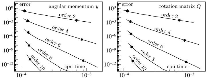
Example 3.1. We consider an asymmetric rigid body with moments of inertia I1 = 0.6, I2 = 0.8, and I3= 1.0 on the interval [0,10]. Initial values arey(0) = (1.8,0.4,−0.9)T andQ(0) is the identity matrix. The
10−4 10−3 10−12
10−9 10−6 10−3 100
10−4 10−3
10−12 10−9 10−6 10−3 100
error
cpu time order 2
order 4
order 6
order 8
orde r
10
angular momentumy error
cpu time order 2
order 4
order 6
order 8
orde r
10
rotation matrixQ
Figure 2. Work-precision diagram for the DMV algorithm (order 2) and for the modifying
DMV integrators of orders 4, 6, 8, and 10.
andC(y) are constant along the numerical solution, we recompute the values ofIej in every step to simulate the presence of an external potential.
We apply the DMV algorithm and its extensions to order 4, 6, 8, and 10 with many different step sizes, and we plot in Figure 2 the global error at the endpoint as a function of the cpu times. The execution times are the average of 1000 experiments. The symbols indicate the values obtained with the step sizes h = 0.1 and h= 0.01, respectively.
The pictures nicely illustrate the expected orders of the algorithms (order pcorresponds to a straight line with slope−p). Much more interesting is the fact that high accuracy is obtained more or less for free. Consider the results obtained with step sizeh= 0.1. The error for the DMV algorithm (order 2) is more than 20%. With very little extra work, the modification of order 10 gives an accuracy of more than 11 digits with the same step size.
References
[1] P. Chartier, E. Hairer, and G. Vilmart. Numerical integrators based on modified differential equations.Submitted for publication, 2006.
[2] K. Feng. Difference schemes for Hamiltonian formalism and symplectic geometry.J. Comp. Math., 4:279–289, 1986.
[3] E. Hairer, C. Lubich, and G. Wanner.Geometric Numerical Integration. Structure-Preserving Algorithms for Ordinary Differ-ential Equations. Springer Series in Computational Mathematics 31. Springer-Verlag, Berlin, second edition, 2006.
[4] E. Hairer and G. Vilmart. Preprocessed Discrete Moser–Veselov algorithm for the full dynamics of the free rigid body.Submitted for publication, 2006.
[5] B. Leimkuhler and S. Reich.Simulating Hamiltonian Dynamics. Cambridge Monographs on Applied and Computational Math-ematics 14. Cambridge University Press, Cambridge, 2004.
[6] R. I. McLachlan. A new implementation of symplectic Runge–Kutta methods.Submitted for publication, 2006.
[7] R. I. McLachlan and A. Zanna. The discrete Moser–Veselov algorithm for the free rigid body, revisited.Found. Comput. Math., 5:87–123, 2005.
[8] J. Moser and A. P. Veselov. Discrete versions of some classical integrable systems and factorization of matrix polynomials. Comm. Math. Phys., 139:217–243, 1991.