Thermal-Economic Optimization of Shell and Tube Heat Exchanger by using a new Multi-Objective optimization method

1. Introduction

Shell and tube heat exchangers are probably the most common type of heat exchangers applicable for a wide range of operating temperatures and pressures. Shell and tube heat exchangers are widely used in refrigerating, power generating, heating and air conditioning, chemical processes, manufacturing and medical applications.

A typical shell and tube heat exchanger is shown in [1, 2]. This widespread use can be justified by its versatility, robustness and reliability. The design of Shell and Tube Heat Exchangers (STHEs) involves a large number of geometric and operating variables as a part of the search for an exchanger geometry that meets the heat duty requirement and a given set of

design constrains. Usually a reference geometric configuration of the equipment is chosen at first and an allowable pressure drop value is fixed. Then, the values of the design variables are defined based on the design specifications and the assumptions of several mechanical and thermodynamic parameters in order to have a satisfactory heat transfer coefficient leading to a suitable utilization of the heat exchange surface. The designer’s choices are then verified based on iterative procedures involving many trials until a reasonable design is obtained which meets the design specifications with a satisfying compromise between pressure drops and thermal exchange performances [1, 2].

Designing the heat exchangers is a complex procedure and it requires a good knowledge of

Thermal-economic optimization of shell and tube heat exchanger using a

new multi-objective optimization method

Mohammad Sadegh Valipour

1

, Mojtaba Biglari

1

, Ehsanolah Assareh

2, *

1_{Faculty of Mechanical Engineering, Semnan University, P.O. Box 35131-19111, Semnan, Iran} 2,*

Department of Mechanical Engineering, Dezful Branch, Islamic Azad University, Dezful,Iran Journal of Heat and Mass Transfer Research 1 (2016) 67-78

Journal of Heat and Mass Transfer Research

Journal homepage: http://jhmtr.journals.semnan.ac.ir

A B S T R A C T

Many studies have been performed by researchers about Shell and Tube Heat Exchanger but the Multi-Objective Big Bang-Big Crunch Algorithm (MOBBA) technique has never been used in such studies. This study presents application of thermal-economic multi-objective optimization of shell and tube heat exchanger using MOBBA. For an optimal design of a shell and tube heat exchanger, it was first modelled thermally using e-NTU method while Bell-Delaware procedure was applied to estimate its shell side heat transfer coefficient and pressure drop. The MOBBA method was applied to obtain the maximum effectiveness (heat recovery) and the minimum total cost as two objective functions. The results of the optimal designs are a set of multiple optimum solutions, called ‘Pareto optimal solutions'. In order to show the accuracy of the algorithm, a comparison is made with the Non-dominated Sorting Genetic Algorithm (NSGA-II) and MOBBA which are developed for the same problem.

© 2016 Published by Semnan University Press. All rights reserved.

PAPER INFO

History:

Submitted 14 January 2014

Revised 24 July 2014

Accepted 19 June 2016

Keywords:

Shell and Tube Heat Exchanger

Multi-Objective Big Bang-Big Crunch Algorithm (MOBBA)

Non-Dominated Sorting Genetic Algorithm (NSGA-II)

Effectiveness

Total cost.

Address of correspondence author:Ehsanolah Assareh, Department of Mechanical Engineering, Dezful Branch, Islamic Azad University, Dezful,Iran.

thermodynamics, fluid dynamics, cost estimation and optimization. The objectives involved in the design optimization of heat exchangers are thermodynamic (i.e. maximum efficiency) and economic (i.e. minimum cost). The conventional design approach for heat exchangers involves rating a large number of different exchanger geometries to identify those designs that satisfy a given heat duty and a set of geometric and operational constraints. This approach is time-consuming, and does not guarantee an optimal solution. [3]

2. Literature Review

Several studies are presented to propose optimization of shell and tube heat exchanger.Min Zhao and Yanzhong Li used an effective layer pattern optimization model for multi-stream plate-fin heat exchanger using genetic algorithm. In this study, an effective layer pattern optimization model using Genetic Algorithm (GA) was developed in detail [4]. Suxin Qian et al. presented applicability of entransy dissipation based thermal resistance for the design optimization of two-phase heat exchangers. In this study, the evaluation of two-phase entransy was achieved by optimizing one tube-fin heat exchanger and one micro channel heat exchanger based on a validated heat exchanger modeling tool [5]. Khaled Saleh et al. applied approximation assisted optimization of headers for a new generation of air-cooled heat exchangers. In this study an online multi-objective approximation assisted optimization approach was used to design optimum headers for compact air-cooled heat exchangers [6]. Amin Hadidi and Ali Nazari used the design and economic optimization of shell-and-tube heat exchangers using Biogeography-Based Optimization (BBO) algorithm. In this research, a new shell and tube heat exchanger optimization design approach was developed based on biogeography-based optimization (BBO) algorithm. The BBO algorithm has some good features in reaching the global minimum in comparison with other evolutionary algorithms [7]. SalimFettaka et al. developed the design of shell-and-tube heat exchangers using multi-objective optimization. In this study, a multi-objective optimization of the heat transfer area and pumping power of a shell-and-tube heat exchanger was presented to provide the designer with multiple Pareto-optimal solutions which captured the trade-off between the two objectives [8]. Sreepathi and G.P. Rangaiah applied an improved heat exchanger network retrofitting using exchanger reassignment strategies and multi-objective optimization. In this study, several ERS (exchanger reassignment strategies) for HEN retrofitting were proposed and tested by performing single objective optimization

tube length, pressure drops and velocities in both sides of the ACHE, heat transfer area and fan power consumption[14].Vivek Patel and VimalSavsani presented optimization of a plate-fin heat exchanger design through an improved Multi-Objective Teaching-Learning Based Optimization (MO-ITLBO) algorithm. In this study, the Multi-Objective Improved Teaching-Learning-Based Optimization (MO-ITLBO) algorithm was introduced and applied for the multi-objective optimization of plate-fin heat exchangers[15]. Costa and Queiroz developed design optimization of shell-and-tube heat exchangers [16]. Caputo et al. presented heat exchanger design based on the economic optimization [17]. Fesanghary et al. applied a harmony search algorithm to design optimization of shell and tube heat exchangers [18]. Hilbert et al. developed parallel genetic algorithms to shape optimization of a heat exchanger [19]. Sanaye and Hajabdollahi used multi-objective optimization of shell and tube heat exchangers [20]. Ponce-Ortega et al. used the genetic algorithms for the optimal design of shell-and-tube heat exchangers [21]. Jie Yang et al. developed optimization of shell-and-tube heat exchangers using a general design approach motivated by constructal theory [22]. Daniël Walraven et al. used optimum configuration of shell-and-tube heat exchangers in low-temperature organic Rankine cycles [23]. Jie Yang et al. developed optimization of shell-and-tube heat exchangers conforming to TEMA standards with the designs motivated by constructal theory [24]. Mohsen Amini and Majid Bazargan used two-objective optimization in shell-and-tube heat exchangers using genetic algorithm [25]. Literature review also indicates that BBA algorithm has never been used for such a study.

2. Mathematical Model for Optimization

of

Shell

and

Tube

Heat

Exchanger

Mathematical model

Based on the work of Sanaye and Hajabdollahi [20], effectiveness of the standards of the Tubular Exchanger Manufactures Association (TEMA) E-type Shell and Tube Heat Exchanger (STHE) is given as the following[20]:

 

  1 2 2 2

1 exp 1

2 1 1

1 exp 1

NTU C

C C

C NTU C

                           _{ }    (1)

Where the number of transfer units (NTU) and the heat capacity ratio (C) are defined as follows [20]:





m in t m in t A A P C m U C U NTU    (2) m ax m in

C

C

C



(3)

Where At is the total tube outside heat transfer

surface area and Uo is the overall heat transfer

coefficient which is computed by the following equation [20]:

t o

t Ld N

A 



(4)

Where L, N t, di, do, Ri,f, R o,f, and kw are the tube

length, tube number, tube inside and outside diameter, tube and shell side fouling resistances and thermal conductivity of tube wall respectively.





, ,

1 / 1 / ln / / 2

1 / ( / )

o o o f o o i w

i f i o i

U h R d d d k

R h d d

  

 

(5)

The tube side heat transfer coefficient is estimated by the following equation [20]:



/



0.024Re

0.8

Pr

0.4

i t i t

h



k

d



5 10 * 24 . 1 Re 2500  t 

(6)

Where kt and Prt are the tube side fluid thermal

conductivity and Prandtl number respectively. Also Ret is the tube flow Reynolds number which is

defined as follows [20]:

t o i t t A d m , Re   (7)

Where mt is the mass flow rate and Ao,t is the tube

side flow cross section area per pass estimated as [20]:

2

, 0.25 /

o t i t p

A 



d N n (8)

And np is the number of tube passes. Furthermore,

the tube side pressure drop is also estimated by the following formula:









 





2 2 2

1 2 / 1

/ 2

4 / 1 / 1 /

c i o

t

t i _m e i o

K p G

f L d K

         _{    }      _{ }        (9)

Where ΔPt includes the pressure drop due to the

flow contraction, acceleration, friction, and expansion, four terms in Eq. (9). Kc and Ke are the

tube entrance and exit pressure loss coefficients. Furthermore ft is the tube side friction factor

estimated as the following [20]:

 

0.311

Re

1143

.

0

000128

.

0







_t

t

f

(10)

The shell diameter is estimated by the following equation:





0.637 /

s t t

D  p N CL CTP (11)

(12)

Where pt is the tube pitch and CL is the tube

layout constant that has a unit value for 45 and 90 tube arrangements and 0.87 for 30 and 60 tube arrangements. Also, CTP is the tube count constant which is 0.93, 0.9, and 0.85 for the single pass, two passes and three passes of tubes, respectively.

Bell-Delaware method is used in this study to compute the shell side heat transfer coefficient and pressure drop. For more information, readers are referred to ref. [20].

3. Entropy Generation Number

The irreversibility losses in the heat exchanger are evaluated in terms of entropy generation. The entropy generation rate caused by the finite temperature difference S_gen,T can be written as follows [26]:     1,2 , , 1 2 , , , ln ln o gen i

s o t o

s i t i

mCpdT S T T T T mCp mCp T T                          



(13)

For an incompressible fluid under non-adiabatic condition the entropy generation rate S_gen,Pcaused by fluid friction is expressed as follows [26]:

1,2

, ,

,

1 2

, ,

1 , 2 ,

ln , ln ln , o i

gen _{o i}

s o t o

t i s o s i t o t i

T T P

S P m

T T

T T

Ts i T

P P

m m

T T T T

       _ _  _{ }                                 _    (14)

The total entropy generation rate in heat exchanger can be written as follows [26] :









,

, 1

1 , ,

,

, , ,

2 1 2

2 , , , ,

ln , , ln ln ln s o s i gen gen gen

s o s i t o

t i s o t o

t o t i s i t i

T T P S S P S T m

T T

T

T T T

P

m mCp mCp

T T T T

                              _{     }      _{   } (15)

When the heat capacity rate of the hot fluid is larger than that of the cold fluid, the outlet temperature of both fluids can be calculated as follows [20]:

) ( _{, ,}

m in ,

, si ti

s i s o

s T T

C C T

T  



 (16)

) ( _{, ,}

m in ,

, si ti

t i t o

t T T

C C T

T  



 (17)

4. Multi-Objective Optimization Problems

Many optimization problems can be presented by the following general mathematical model [27]:

Max. /Min. F (x) xϵ X (18)

F: X → R (19)

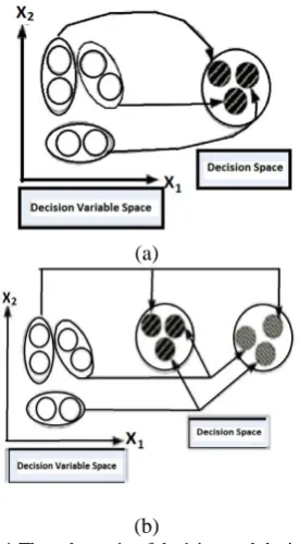
In which f(x) is the objective function, x is the decision variables vector, X is the decision variables space, and R is the set of real numbers.

Figure (1-a) shows a schematic of transferring data from a two dimensional decision variable space to a decision space in single objective problems. In multi-objective optimization problems, optimizing a vector of objectives is considered instead of satisfying a single objective.

Generally, in mathematical form, multi-objective optimization problems can be defined as follows [27]:

Max. /Min f(x) = (f1(x), f2(x)… fm(x))

xϵ X

(20) F: X → Rm_{, mϵ M}

(21) Where m denotes the set of natural numbers and N denotes the number of objectives. There are techniques such as the weighting method and Ɛ -constraint method which transfer multi-objective problems to a single-objective one using different combinations of a weighting vector and constraints. Thus, each optimal solution can be assigned to a specific combination of weighting vector and constraint. Hence, in each run of the algorithm, a single point (solution) can be achieved. However, multi-objective evolutionary algorithms are capable of finding almost all candidate solutions (Pareto) in a single run.

Figure (1-b) presents a schematic of transferring data from two dimensional decision variables space to the decision space in a two-objective problem.

As it is shown, each set of decision variables has been related to a couple of objectives. Note that none of the solutions dominates the others. In other words, if all the objective values of a solution dominate the corresponding values of another solution, the former will be a dominated solution and the latter will be removed. Otherwise, both solutions will be located in the non-dominated set.

The dominated and non-dominated relations between objectives values in a bi-objective problem are shown in Fig.2.Both objectives are minimized. In this figure, the solutions labeled by 1 or 2 have non-dominated conditions individually. We should note that the set labeled 1 dominates the set labeled 2. In the optimization procedure, the best set of non-dominated solutions is called Pareto-front. Thus, there are two Pareto in Figure (2), and the one which is labeled 1 is the Pareto-front. [27]

 

o s o

Sd u d

G _



(a)

(b)

Fig. 1 The schematic of decision and decision variable spaces in: (a) single-objective and (b)

multi-objective problems.

Fig.2 The schematic of dominated and non-dominated conditions of solutions in a projective problem.

The analogy of Big Bang - Big Crunch Algorithm (BB-BCA) with evolutionary algorithms makes it evident that using a Pareto ranking scheme [28] could be the straightforward way to extend the approach to handle the multi-objective optimization problems. The historical record of the best solutions found by a particle (i.e., an individual) could be used to store non-dominated solutions generated in the past (this would be similar to the notion of elitism used in evolutionary multi-objective optimization). The use of global attraction mechanisms combined with a historical archive of previously found non-dominated vectors would motivate convergence toward globally non-dominated solutions.

5. Big Bang-Big Crunch Algorithm (BBA)

In the BB-BC algorithm proposed by Erol and Eksin[29], the initial big-bang is identical to the first step of the other evolutionary methods in that an initial population of candidate solutions is randomly generated over the entire search space. Erol and

Eksin compared this random nature of the Big Bang to the energy dissipation or the transformation from an ordered state (a convergent solution) to a chaotic state (generation of new set of candidate solutions). In the Big Crunch phase following the Big Bang, a contraction operation is applied to randomly distributed candidate solutions. The contraction operator takes the current positions (represented by the values of the design variables) of each candidate solution in the population and its corresponding penalized fitness function value to compute a center of mass. The center of mass is the weighted average of the candidate solution positions where the weight associated with the position of each candidate solution is the inverse of the corresponding penalized fitness function. The averaging is done with respect to the inverse of the penalized fitness function values. The center of mass 𝑋⃗𝑐𝑚 is computed as the following [29]:

𝑋⃗𝑐𝑚=

∑ 𝑋⃗⃗𝑘 𝐹_𝑘 𝑁𝐶 𝑘=1

∑ 1

𝐹𝑘 𝑁𝐶

𝑘=1 (22)

Where X⃗⃗⃗k is the position of candidate k in an

n-dimensional searchspace, Fk is the penalized fitness function value of candidate k, and NC is the candidate population size. New positions X⃗⃗⃗_knewof the candidate solutions for the next iteration of the Big Bang are obtained using the following equation [29]:

𝑋⃗𝑘𝑛𝑒𝑤 = 𝑋⃗𝑐𝑚+ 𝜎⃗ (23)

Where σ⃗⃗⃗ is the standard deviation of the normal distribution. In the BB-BC algorithm, the standard deviation σ⃗⃗⃗is related to asubset of search space and is obtained by the following equation [29]:

𝜎⃗ =𝑟 ∝1(𝑋⃗𝑚𝑎𝑥− 𝑋⃗𝑚𝑖𝑛) 𝑛𝑐𝑦𝑐𝑙𝑒

(24)

Where r is a random number from a standard normal distribution, ∝₁ is a parameter limiting the size of the search space, X⃗⃗⃗maxand X⃗⃗⃗⃗min are the upper

and lower limits of the values of the design variables respectively, and n_cycle is the number of Big Bang iterations.

A modified version of Eq. (23) is given as follows [29]:

𝑋⃗𝑘𝑛𝑒𝑤

=∝2𝑋⃗𝑐𝑚

+ (1 −∝2)[∝3𝑋⃗𝑙𝑏𝑒𝑠𝑡

+ (1 −∝3)𝑋⃗𝑔𝑏𝑒𝑠𝑡]

+𝑟 ∝1(𝑋⃗𝑚𝑎𝑥− 𝑋⃗𝑚𝑖𝑛) 𝑛𝑐𝑦𝑐𝑙𝑒

(25)

Where ∝2, ∝3 are thecontrolling parameters,

X⃗⃗⃗lbest is the local best solution,and X⃗⃗⃗gbest is the global

best solution. Since normally distributednumbers can exceed ±1, it is necessary to limit candidate positions to the prescribed search space boundaries. As a result of this contraction, there is an accumulation of candidate solutions at the search space boundaries.

In Eq. (25) ∝₁, ∝₂ and ∝₃ are the adjustable parameters that control the influence of the local and the global best solutions on the new positions of candidate solutions.

In addition, the BB-BC algorithm employs a multiphase search. In a two-phase search, the BB-BC algorithm is initially applied to the entire search space. After the convergence of Phase I, the Phase II search starts in a reduced search around X⃗⃗⃗best from Phase I. The search space is reduced to 20% of the original search space [30].

6. EconomicModelling

The total cost of the STHE heat exchanger is given by the following [20]:

in op tot C C

C   (26)

Where Cin and Cop are the total investment cost

and the operating cost of the heat exchanger respectively and are defined as follows [20]:



el

pk co

0.85 in 8500 409

C   A

(27)

 

1

( _{t t t s s s})

p mp   m p   (28)

Where ny is the equipment life in year, i is the

annual discount rate and k is the depreciation time in year. Also, ΔP and m are the pressure drop and the mass flow rate of the fluid. Cop is the annual operating cost and it is calculated as follows:



 

 ny

k

k i co Cop

1 /(1 )

(29)

Where kel, τ and ɳp are the electricity unit cost,

the operation hours of the heat exchanger per year and the pump efficiency respectively. The detailed calculation of different parameters of the above mentioned equations is given in Refs. [20, 26].

7. Case Study

The analysis of the case study has been performed by Sanaye et al. [20] using NSGA-II approach according to the literature [2]. The original design specifications, shown in Table (1), are fed as inputs into the MOBBA algorithm.

In Figure (3), the optimal heat exchanger architectures obtained by MOBBA are compared with those of Sanaye et al. [20] using the NSGA-II approach and also with the original design solution given by Shah et al. [2].

The application example of STHE was also analysed to ensure the capability of MOBBA which was earlier analysed using NSGA-II by Sanaye and Hajabdollahi [20]. With the help of fresh water, the oil cooler STHE used to lower the temperature of the oil was designed and optimized for providing the maximum effectiveness and the minimum total cost. The high temperature of oil with mass flow rate of 8.1 kg/s was poured into the shell side of STHE at a temperature of 78.3 ºC. Also, the fresh water with mass flow rate of 12.5 kg/s at a temperature of 30 ºC was poured into the tube side of STHE. The thermo physical properties of both the fluids were taken from Ref. [20].

The following inequality constraints which are bound by lower and upper limits of the design variables are considered in the present study and three different tube arrangements (30º, 45º and 90º) are also considered for the optimization.

0.0112 ≤ di ≤ 0.0153 1.25 ≤ pt/do ≤ 2

3 ≤ L ≤ 8

100 ≤ Nt ≤ 600

0.19 ≤ bc/Ds ≤ 0.32

0.2 ≤ bs/Ds ≤ 1.4

3 ≤ L/Ds ≤ 12

In this study, the following assumptions were made:

 Price of electricity (kel) : 0.15 $/kWh,

 Equipment life period (ny) : 10 years

 Annual discount rate (i) : 10%,

 Hours of operation per year (s) : 7500 h/yr

 Pump efficiency (η) : 0.6

Table1. The process input and physical properties for different case studies"

Properties Pr K(W/m2

.K) Cp(j/kg.K) µ(Pa.s) Rf

Shell side 966 0.14 2115 0.0643 0.00015

Fig.3 Theoptimized point's distribution in pareto by using MOBBA

8. Distance Criterion

The distance criterion measures (d) cover and give distribution to the proposed space. In this study, the distance criterion is used to compare the results of two algorithms, MOBBA and NSGA-II. The result is discussed in section 9.

2

1( )

1 /

1 



_ 

 n

i d di n

d (30)

n

j

i

,



1

,....,

(31)

Also, using di , we can find the minimum point distance of the diagram based on the ideal point using such criterion [20].

9. Optimization Results

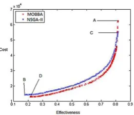
The numbers of iterations for finding maxima or minima, in the search space are almost 104 and the number of populations and repositories are 100. The results are shown in figure (4) via the Pareto diagram. The figure demonstrates clearly the presented differences between both objective functions.

Increasing heat transfer in the heat exchanger, the total cost would increase. So, we use multi- objective optimization method for shell-tube heat exchanger to decrease the cost. Figure (6) shows the minimum amounts of total cost with the least effectiveness. Here, the MOBBA algorithm results are compared with the results of the NSGA- II algorithm previously proposed by Mr. Sanaye in 2010 [20].

We use distance criterion for comparing the results of two algorithms, MOBBA and NSGA-II, which this scale is 0.3919 for the NSGA-II algorithm and 0.3112 for the MOBBA algorithm. These amounts indicate that the point achieved by the MOBBA algorithm is closer to the ideal point rather than the point achieved by the NSGA-II algorithm. Figure (4) shows a better performance of the MOBBA algorithm compared to the NSAG- II algorithm.

For both algorithms in the figure (3), A and C points are happened when optimization is done as a single objective and so our objective functions are

maximization of the effectiveness. For B and D points, our objective functions are minimization of the total cost. Figures (5) and (6) are related to the maximum effectiveness and minimum total cost, respectively. It is obvious that for the total cost, the results in the MOBBA algorithm are optimized to 7.36 % and so for Q maximum, the MOBBA algorithm has better results than the NSGA-II.

10. External Temperatures

According to the equations (16) and (17) the relations for external temperatures of heat exchanger and the amounts of these temperatures are obtained based on the limitation of the total cost, effectiveness and decision variables in figure (3) for both algorithms in the figures (8) to (10).

These figures emphasize the problem that there is an external temperature in the tube for an external temperature in the shell with the optimized amounts of decision variables. The maximum amounts of effectiveness in (16) and (17) equations are accompanied with the minimum amounts for external temperature of the shell, and the maximum external temperature of the tube.

Also, the optimized amount of the external temperature in the tube is 63.85 for the MOBBA algorithm and for the external temperature of the shell is 44.440C

11. Entropy Balance

Figure (11) and figure (12) show the entropy amounts based on the effectiveness and also show the total cost for highlighted points in figure (3).

Figure (11) shows the entropy amount based on the output heat. More specifically, it shows that the amount of system entropy increases with increasing the output.

Also, figure (12) shows incurred cost increased with increasing the output. For the amount of the best optimized point, which is obtained by pareto diagram in figure (3) for the MOBBA algorithm, the amount of effectiveness is 0.7051 and the cost is 28184 $ and the amount of produce entropy cost is 29287.

12. Conclusion

Designing the heat exchanger can be a complicated task. Thus, the advanced optimization methods are useful for identifying the best and cheapest heat exchanger for a specific duty. In this study, the shell and tube heat exchanger design and the multi-objective optimization are performed with the MOBBA algorithm. The results are compared with those of Sanaye paper [20]. The MOBBA algorithm is a useful method for the shell and tube heat exchanger design and optimization. These results are demonstrated in similar conditions for two-objective functions (effectiveness and total cost)





 



 M

m

j m i

m i

i f x f x

d

1 ( ) ( )

and indicate that the MOBBA is a better and more effective method than the NSGA-II algorithm. The algorithm proposed here can help the manufacturer and engineers to optimize heat exchangers in engineering applications.

Fig. 4 The related results to D criterion for the MOBBA & NSGA-II.

Fig. 5 The comparison of the maximum effectiveness for the MOBBA& NSGA-II[8].

Fig. 6 The comparison of the least total cost for MOBBA& NSGA-II [8].

Fig. 7 The comparison of the maximum heat transfer for the MOBBA& NSGA-II [8].

Fig. 8 The external temperature based on effectiveness for the MOBBA& NSGA-II [8].

Fig. 9 The comparison of the maximum tube external temperature for the MOBBA& NSGA-II [8].

Fig. 10 The comparison of the least shell external temperature for the MOBBA & NSGA-II [8].

Fig. 12 The entropy balance based on total cost for the MOBBA.

Nomenclature

A heat transfer area (m2₎

BC baffle cut (m)

Cp specific heat in constant

pressure

(J/kg K)

C heat capacity rate ratio (Cmin/Cmax)

Cin total investment cost ($)

Cop total operating cost ($)

Co annual operating cost ($/yr)

Ctotal total cost ($)

CL tube layout constant (-)

CTP tube count calculation

constant

(-)

di tube side inside diameter (m)

do tube side outside diameter (m)

Ds shell diameter (m)

f friction factor (-)

Gs fluid mass velocity based on

the minimum free area

(kg/s.m2₎

hi tube side heat transfer

coefficient

(W/m2 _K)

ho shell side heat transfer

coefficient

(W/m2 _K)

i annual discount rate (%) jc correction factor for baffle

configuration

js correction factor for bigger

baffle spacing at the shell inlet and outlet sections jr correction factor for the

adverse temperature gradient in laminar flows

jb correction factor for bundle

and pass partition bypass streams

jl correction factor for baffle

leakage effect

Kc entrance pressure loss

coefficient

(-)

Ke exit pressure loss coefficient (-)

kel price of electrical energy ($/kWh)

k thermal conductivity (W/m k)

L tube length (m)

Lbc baffle spacing (m)

m mass flow rate (kg/s)

np _{number of tube pass} (-)

Nt number of tube (-)

NT

U number of transfer units

(-)

Pt tube pitch (m)

Q heat transfer rate (kW)

Re Reynolds number (-)

T temperature (o_C)

U overall heat transfer (W/m2 _K)

coefficient

σ ratio of minimum free flow area to frontal area

(-)

P pumping water (W)

𝜎 ratio of minimum free flow area to frontal area

(-)

ρ density (kg/m3₎

Sub scri pts

i= input O= output

References

[1] G.F.Hewitt, editor. Heat exchanger design handbook. New York: Begell House; (1998).

[2] R.K. Shah, Bell KJ. The CRC handbook of thermal engineering. CRC Press; (2000).

[3] V. Rao, V. Patel, Multi-objective optimization of heat exchangers using a modified teaching-learning-based optimization algorithm, Applied Mathematical Modeling, 37(3), 1147-1162, (2013).

[4] Min Zhao , Yanzhong Li,An effective layer pattern optimization model for multi-stream plate-fin heat exchanger using genetic algorithm, International Journal of Heat and Mass Transfer, 60, 480–489, (2013).

[5] Suxin Qian, Long Huang, Vikrant Aute, Yunho Hwang, ReinhardRadermacher, Applicability of entransy dissipation based thermal resistance for design optimization of two-phase heat exchangers. Applied Thermal Engineering, 55, (1), 140–148, (2013).

[6] KhaledSaleh, Omar Abdelaziz, Vikrant Aute, ReinhardRadermacher, ShapourAzarm, Approximation assisted optimization of headers for new generation of air-cooled heat exchangers. Applied Thermal Engineering, 61(2), 817–824, (2013).

[7] Amin Hadidi, Ali Nazari, Design and economic optimization of shell-and-tube heat exchangers using biogeography-based (BBO) algorithm. Applied Thermal Engineering, 51(1), 1263–1272, (2013).

[8] Salim Fettaka, Jules Thibault, Yash Gupta. Design of shell-and-tube heat exchangers using multiobjective optimization. International Journal of Heat and Mass Transfer, 60, 343–354, (2013).

[9] Bhargava Krishna Sreepathi, G.P. Rangaiah, Improved heat exchanger network retrofitting using exchanger reassignment strategies and multi-objective optimization. Energy Available online 24 February 2014 In Press, Corrected Proof.

[10] Viviani C. Onishi, Mauro A.S.S. Ravagnani, José A. Caballero, Mathematical programming model for heat exchanger design through optimization of partial objectives, Energy Conversion and Management, 74, 60– 69, (2013)

[12] R. VenkataRao ,Vivek Patel, Multi-objective optimization of heat exchangers using a modified teaching-learning-based optimization algorithm. Applied Mathematical Modelling, 37(3), 1147–1162, (2013).

[13] Ming Pan, Igor Bulatov, Robin Smith, Jin-Kuk Kim, Optimisation for the retrofit of large scale heat exchanger networks with different intensified heat transfer techniques. Applied Thermal Engineering, 53( 2) , 373– 386, (2013).

[14] Juan I. Manassaldi , Nicolás J. Scenna, Sergio F. Mussati, Optimization mathematical model for the detailed design of air cooled heat exchangers. Energy, 64, 734–746, (2014)

[15] Vivek Patel, Vimal Savsani, Optimization of a plate-fin heat exchanger design through an improved multi-objective teaching-learning based optimization (MO-ITLBO) algorithm. Chemical Engineering Research and Design, Available online 11 February 2014 In Press, Accepted Manuscript.

[16] L.H. Costa, M. Queiroz, Design optimization of shell-and-tube heat exchangers, Applied Thermal Engineering, 28, 1798-1805,(2008).

[17] A. Caputo, P. Pelagagge, P. Salini, Heat exchanger design based on economic optimization, Applied Thermal Engineering, 28(10), 1151–1159, (2008).

[18] M. Fesanghary, E. Damangir, I. Soleimani, Design optimization of shell and tube heat exchangers using global sensitivity analysis and harmony search algorithm, Applied Thermal Engineering, 29, 1026–1031, (2009).

[19] R. Hilbert, G. Janiga, R. Baron, D.Venin, Multi-objective shape optimization of a heat exchanger using parallel genetic algorithms, International Journal of Heat and Mass Transfer,49(15–16), 2567–2577, (2006).

[20] S. Sanaye, H. Hajabdollahi, Multi-objective optimization of shell and tube heat exchangers, Applied Thermal Engineering, 30(14–15), 1937–1945,(2010).

[21] J. Ponce-Ortega, M. Serna-González, A. Jiménez-Gutiérrez, Use of genetic algorithms for the optimal design

of shell-and-tube heat exchangers, Applied Thermal Engineering, 29(2–3), 203–209,(2009).

[22] Jie Yang, Sun-Ryung Oh, Wei Liu,Optimization of shell-and-tube heat exchangers using a general design approach motivated by constructal theory.International Journal of Heat and Mass Transfer,Volume 77, October 2014, Pages 1144–1154.

[23] DaniëlWalraven, Ben Laenen, William D’haeseleer,Optimum configuration of shell-and-tube heat exchangers for the use in low-temperature organic Rankine cycles.Energy Conversion and Management. Volume 83, July 2014, Pages 177–187.

[24] Jie Yang, Aiwu Fan, Wei Liu, Anthony M. Jacobi.Optimization of shell-and-tube heat exchangers conforming to TEMA standards with designs motivated by constructal theory.Energy Conversion and Management.Volume 78, February 2014, Pages 468–476.

[25] Mohsen Amini, MajidBazargan.Two objective optimization in shell-and-tube heat exchangers using genetic algorithm.Applied Thermal Engineering.Volume 69, Issues 1–2, August 2014, Pages 278–285.

[26] R.K. Shah, P.Sekulic, Fundamental of Heat Exchanger Design, John Wiley & Sons, Inc, (2003).

[27] E. Mehdipour, O. Haddad, M. Tabari, M. Mari. Extraction of decision alternatives in construction management projects: Application and adaptation of NSGA-II and MOPSO, Expert Systems with Applications, 39(3), (2012).

[28] D. E. Goldberg, Genetic Algorithms in Search, Optimization and Machine Learning, Reading, MA: Addison-Wesley, (1989).

[29] Osman K. Erol, Ibrahim Eksin,A new optimization method: Big Bang–Big Crunch, Advances in Engineering Software, 37( 2), February 2006, Pages 106–111.