Development of an Efficient Hybrid Method for Motif Discovery in DNA Sequences

63

Development of an Efficient Hybrid Method for Motif

Discovery in DNA Sequences

Reza Akbari

i*

; Vahid Zeighami

ii

; Koorush Ziarati

iii

and Ismail Akbari

iv

A

BSTRACT

This work presents a hybrid method for motif discovery in DNA sequences. The proposed method called

SPSO-L

k

, borrows the concept of Chebyshev polynomials and uses the stochastic local search to improve the

performance of the basic PSO algorithm as a motif finder. The Chebyshev polynomial concept encourages

us to use a linear combination of previously discovered velocities beyond that proposed by the basic PSO

algorithm. Under this method, to balance between exploration and exploitation, at each iteration step, a local

region is associated with each candidate particle, and a local exploration performed in this blob. The

stochastic local search employs an intelligent repulsion/attraction mechanism to navigate a particle to

explore this local region beyond that defined by the search algorithm to achieve a better solution. Over the

successive iterations, the size of local region dynamically decreases. Also a non-linear dynamic inertia

weight is introduced to further improve the performance of SPSO-L

k

approach. The SPSO-L

k

is tested on

different sets of simulated and real nucleotide sequences to discover implanted DNA motifs. Experimental

results show that the SPSO-L

k

is effective, and provides competitive results in comparison with the

performance of other algorithms investigated in this consideration.

K

EYWORDS

Particle Swarm Optimization, Stochastic Local Search, Motif Discovery

i *Corresponding Author, Reza Akbari is with the Department of Computer Engineering and Information Technology, Shiraz University of Technology, Shiraz, Iran, (email: [email protected])

ii Vahid Zeighami is with the Department of Mathematics and Industrial Engineering, Ecole Polytechnique, de Montreal, Montreal, Quebec, Canada, (email: [email protected])

iii Koorush Ziarati is with the Department of Computer Science and Engineering, Shiraz University, Shiraz, Iran, (email: [email protected]) ivIsmail Akbari is a graduated student from Department of Industrial Engineering, Iran University of Science of Science and Technology, Tehran, Iran, (email: [email protected])

1.INTRODUCTION

Discovering motifs in DNA datasets has been the focus of many recent researches in bioinformatics. DNA motifs are structural patterns that occur frequently in a set of nucleotide sequences. Sometimes, these motifs directly determine the functions of the sequences in which they occur. So, discovering the structural motifs in DNA datasets plays an important role in bioinformatics area ‎[1]. The task of motif discovery can be defined as the searching of the motifs that meet the predefined format and criteria. It is assumed that the motifs themselves and the existence of the motifs are not known a priori. Motif discovery is a search problem. So many search methods such as genetic algorithms, particle swarm optimization, local searches and etc. can be applied to discover planted

 

l

,

d

-motifs ‎[1]. In recent years many algorithms for finding

 

l

,

d

-motif in biological sequences are proposed.

Exhaustive search such as Suffix tree ‎[1], WEEDER ‎[2],

and MITRA ‎[3] are of the first algorithms used to find

 

l

,

d

-motifs in biological sequences. Heuristic Based algorithm such as CONSENSUS ‎[4] is another type of the algorithms for this problem. Other Machine learning algorithms such as Expectation Maximization (MEME) ‎[5], Gibbs Sampling ‎[6], Genetic Algorithms ‎[7], etc. are used to discover unknown motifs in biological sequences. Also many other algorithms are presented in the literatures ‎[8]-‎[19].

unique to a family of proteins.

In this paper, we present a new hybrid algorithm based on particle swarm optimization and stochastic local search for identification of

 

l,d motifs in given DNA sequences. The algorithm computes linear combinations of previous velocities of the particles and previous best positions to significantly improve the performance of the original algorithm. Stagnation and Premature convergence are two of the main deficiencies of the original PSO algorithm ‎[25]. In this paper, we use the stochastic local search to mitigate premature convergence problem. To cope with stagnation, a new method called repulsion/attraction mechanism is introduced. Also, a new non-linear adaptive inertia weight is introduced to further improve the performance of the proposed method.

The rest of the paper is organized as follows. Section 2 introduces the concepts of the original Particle Swarm Optimization. Section 3 defines basic concepts of the Stochastic Local Search. Description of the proposed algorithm is presented in section 4. The adaptation of the proposed algorithm for motif discovery in a set of DNA sequences is presented in Section 5. Also, this section reports experimental analysis on the proposed algorithm. Finally, section 6 concludes the paper.

2. PrinciplesofParticleSwarmOptimization ‎[20]

The original PSO algorithm is an iterative process in which a set of particles, are characterized by their position and the velocity with which they move in the solution space of a cost function. Each individual in PSO flies in the parameter space with a velocity which is dynamically adjusted according to the flying experiences of its own and those of its companions. Therefore, every individual is gravitated toward a stochastically weighted average of the previous best point of its own and that of its neighborhood companions. Mathematically, given a swarm of particles, each particle is associated with a position vector, which is a feasible solution for an optimal problem; let the best previous position (the position giving the best objective function value called pbest) that the i-th particle has found in the parameter space be denoted by pi; the best position that the neighborhood particles of the i-th particle have ever found called gbest is denoted by gi. At the start time all of the positions and velocities are initialized randomly. At each iteration step, the position vector of the particle, is updated by adding an increment vector. In the original PSO algorithm, the particles’ positions are updated according to the following equations ‎[20]:

 

 



 



 



g x t



r c t x p r c t v t v i d i d i d i d i d i d           2 2 1 1 1 (1)

 





 

 





            max max max max 1 1 1 v t v if v v t v if v t v _i d i d i

d (2)

 

t1 x

 

t v

 

t1

x id

i d i

d (3)

where v

 

t1 is the velocity vector, which controls the

amount of increment of the position of a particle, x

 

t1

is the next position of the particle,

v

_max is a maximum

velocity possible for particle,

c

₁ and

c

₂ are two positive constants which control the importance of the individual knowledge and that of the neighbors, rand₁ and rand₂

are two random parameters of uniform distribution in range [0, 1], which limit the velocity of the particle in the coordinate direction.

This iterative process will continue swarm by swarm until a stop criterion is satisfied, and this forms the basic iterative process of a PSO algorithm. In the right-hand side of (1), the second term represents the cognitive part of a PSO algorithm at which the particle changes its velocity based on its own thinking and memory, while the third term is the social part of a PSO algorithm at which the particle modifies its velocity based on the adaptation of the social-psychological knowledge. Based on these formulations, only the best particle in the neighborhood has an impact on the candidate particle. Essentially, the PSO algorithm is conceptually very simple, and can be implemented in a few lines of computer codes. Also, it requires only primitive mathematical operators and very few algorithm parameters need to be tuned.

3.PRINCIPLES OF STOCHASTIC LOCAL SEARCH ‎[24]

Many combinatorial optimization problems with high computational complexity exist. There exist no exact algorithms that can solve instances of these problems within a reasonable time limit. In these cases many successful optimization algorithms use local search techniques with randomized choices and probabilistic decisions to produce or select candidate solutions from the search space ‎[24]. Stochastic local search algorithms are flexible, robust and provide excellent results in many application areas.

Given a problem , a stochastic local search for solving arbitrary instance  is formalized as follows. First we describe the required parameters of the algorithm:

1. S

 

 : is the search space for a problem . 2. S'

   

 S : is a set of candidate solutions. 3. sS'

 

 : is a candidate solution.

4. N

 

 : is a neighborhood relation on S

 

 , where N

     

 S S .

65 The objective of an SLS algorithm is to find a solution

by searching in the search space S

 

 . Using the parameters, the algorithm is performed in three steps to find a solution:

1. Initialization: At the first step, an initialization function init

 

 D



S

 

 M

 





selects the start

point for the algorithm in the search space. Usually, a random approach is used to find this point. In fact, the probability distribution over initial search position and memory states are specified.

2. Iterative improvement: After initialization, the

step function

   

 S M

 

 D



S

 

 M

 





step :    is applied

to replace the current solution s with a better candidate solution from the neighborhood of s

while replacing the memory state m with the corresponding new memory state. The step function maps each search position and memory state onto the probability distribution over the subsequent, neighboring search position and memory states. The set of probability distribution over a given set S is denoted by D

 

S . A probability distribution DD

 

S is a function

] 1 , 0 [ :S

D with



 



 S s

S D 1.

3. Termination: The step

 

 function is applied iteratively until the termination predicate

 



terminate returns a true value. The function

   

S M

 

D



 

T F



terminate :     ,

determines the termination probability for each search position and memory state.

After terminating the search, the stochastic local search method returns the solution sS'

 

 or it may return “no solution”. In combinatorial approach, where a local search is used to improve the main method, the solution

 

 '

S

s , if exists, contains a better result in comparison with the current best solution.

Here, we used stochastic local search in the SPSO-Lk algorithm to escape from local optima. The proposed algorithm uses randomized choices in generating new solutions in the neighborhood of the candidate solutions. The next search position is selected from the local neighborhood based on local information.

4.THE PROPOSED ALGORITHM

In this section, the variations on the original PSO are described. The variations continuously improve the performance of the original algorithm. In our previous work, a variant of the algorithm was used for optimizing multimodal functions ‎[25]. The SPSO-Lk aims to cope with stagnation problem of the original PSO and to provide a better mechanism for balancing between

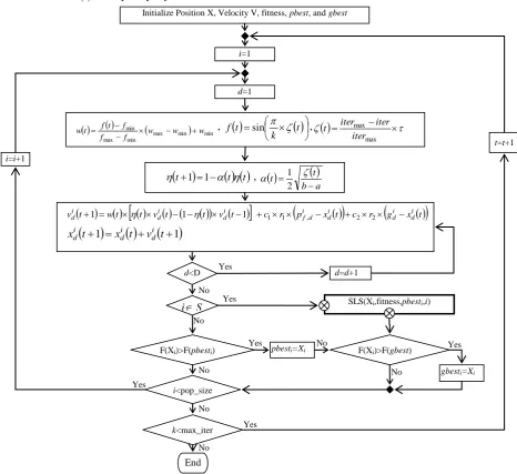
exploration and exploitation. The schematic diagram of the SPSO-Lk algorithm is represented in Figure 1.

During the first step of our algorithm, the required parameters such as population size, the coefficients, initial radius of blobs, number of particles influenced by stochastic local search are determined. After that, the initial values for positions and velocities of particles are randomly generated in the search space. The initial best position of a particle is set to its initial position. The initiation step starts the algorithm.

During each iteration, the velocities of the particle are updated based on a new velocity equation. The velocity equation used here acts like Chebyshev polynomials ‎[26]. More precisely, unlike the original PSO, the two previously discovered velocities used here to compute the new velocity. Using this mechanism mitigates the stagnation problem.

The value of velocity encourages the target particle to transit to the new interesting position. The new positions of the particles are updated using the velocity vectors. A different scenario is introduced here for updating the position of a particle. In this scenario, a particle transition is affected by a stochastic local search to discover better positions.

An individual in the SPSO-Lk algorithm performs a global move followed by one or more local moves. The global move aims to increment the position of a particle using individual and social knowledge. The local move is designed to explore the regions of the search space which are not considered by the global move. As shown in Figure 1, the local move is performed by the SLS function. Since the algorithm is faced with global and local moves, we need to propose a robust combination approach to achieve useful moves. The following subsections describe the details of the algorithm.

A. Update Velocities

Using the previous velocities in iterations t and t-1, the new velocity of each particle is computed using the following equation:

     



 



 



 



 



p x t



c r



g x

 

t



r c t v t t v t t w t v i d i d i d i d f i d i d i d                 2 2 , 1 1 1 1

1  

(4)

where 

 

t is a non-linear function which determines the relative importance of the current and previous velocity vectors. The coefficient 

 

t is dynamically adjusted according to the following equation:

 

t 

   

tt

 1 1 (5)

The coefficient 

 

t is adaptively adjusted as:

 

 

a b t t     2 1 (6) with

 

     max max iter iter iter

t (7)

where t is defined as a linear function, iter is the current iteration; iter_max represents the maximum number of

iterations, a and b respectively represent the upper bound and lower bound values used to control the relative importance of the current and previous velocities, and the parameter 01 transforms the value of t to the range [0, ], here we set  1.

Figure 1: Schematic diagram of SPSO-Lk algorithm. The algorithm combines and improved version of PSO and the stochastic local search. The velocity update equation is similar to Chebyshev polynomials. A non-linear inertia weight improves the balance between global and local search ‎[32].

No No Yes Yes Yes No No No No Yes Yes No Yes

Initialize Position X, Velocity V, fitness, pbest, and gbest

End

k<max_iter

t=t+1 i=1

     

t wt



t v

 

t



 

t



v

 

t



c r



p x

 

t



c r



g x

 

t



v di

i d i d i d f i d i d i

d 1   1  1  1 1 ,   2 2 

 

t1 x

 

t v

 

t1

x di

i d i

d

d=1

d<D d=d+1

i<pop_size i=i+1

F(Xi)>F(pbesti) pbesti=Xi F(Xi)>F(gbest)

gbesti=Xi SLS(Xi,fitness,pbesti,i)

S i

     max min min min

max

min _{w w w}

f f f t f t

w   

   ,

 

 

        t k t

f sin   ,

 

   max max iter iter iter t

 

t 

   

tt

67 Another improvement may be achieved through

acceleration coefficients ‎[27], ‎[28]. Different experiments were carried out to investigate the behavior of the swarm under different settings of the acceleration coefficients. The experiments are performed under fixed, linearly decreasing and non-linearly decreasing acceleration coefficients. Our empirical study showed that the acceleration coefficient c1 and c2 with a fixed value of 1.5 has a better performance than others.

B. Non-Linear Inertia Weight

PSO is a powerful method for finding global optima in optimization area, but it has some deficiencies which should be resolved to achieve better performance. Premature convergence is one of the main deficiencies of the original PSO. The premature convergence usually occurred due to improper balancing mechanism between exploration and exploitation. One solution to mitigate this problem is achieved through inertia weight. The inertia weight may provide proper balancing mechanism. The inertia weight introduces the preference for the particle to continue moving in the same direction it was going on the previous iteration. At the first iterations the exploration is preferred and the exploitation is preferred at the last iterations. Broad considerations on inertia weight are performed and many improvements are presented. Eberhart and Shi ‎[23] found that linearly decreasing inertia in not very effective in dynamic environments. A non-linear inertia weight provides more flexibility to control the balance between exploration and exploitation throughout iterations.

SPSO-Lk algorithm uses a non-linear and dynamic inertia weight ‎[32]. The inertia weight is based on a non-linear sinusoid function f :

 

 



  

  

 t

k t

f sin   (8)

where k is a constant factor, in all our experiments the SPSO-Lk algorithm uses parameter k2. The parameter t is defined in (7); here the value of  is set to 0.5. The behavior of the inertia weight is controlled by adjusting the parameters k and t. These parameters result a wide range of behavior from near linear to periodic with multiple minimum and maximum values.

A sinusoid function generates the data in range of [-1, 1]; so we need to transform them to a predefined range. The max-min normalization is used to perform linear transformation on the data produced by the function. By this transformation the inertia weight factor w is set to

change nonlinearly according to the following equation:

 

 



max min



min

min max

min _{w w w}

f f

f t f t

w   

 

 (9)

Where w_min and w_max respectively represent the minimum and maximum values of the inertia weight. The minimum and maximum values of the function is represented by f_min and f_max . In our experiments w_minis set to 0.4, while w_max is set to 0.9. Adjusting this sinusoid inertia weight with the previously described values results a non-linear decreasing coefficient that improves significantly the performance of the original PSO.

C. Update Positions

The proposed non-linear inertia weight and velocity update equation are used to obtain the next positions of the particles. Here, we have used a different approach to update the positions. Let P be the set of particles constitute the main swarm. The main swarm is partitioned to the sub-swarms U and T (i.e. PUT and

 

T

U ), where T represents the particles which perform the stochastic local search around themselves, while the U represents the other particle with traditional update approach. The U and T are dynamic sets and their members are updated throughout iterations. Different ways can be used to define the members of the sets U and T. In one way, the particles are sorted based on their fitness, and

k best particles are selected as members of the set T. The remainder particles constitute the set U. In other way, the k

members of set T are selected randomly. Parameter k can be static or dynamic. In static fashion, a predefined percent k n of particles contribute in stochastic local

search, where n is the number of particles, while in dynamic fashion parameter k can obtain different values throughout iterations. Based on these considerations, each particle modifies its position according to the following equation:

 

 



 

 

 



   

 



 

 



T i iff t

v t x SLS

U i iff t

v t x t

x _i

d i d

i d i d i

d

1 1

1 (10)

Figure 2: Local landscape around a particle may provide valuable information which is not considered by the PSO. The velocity update equation would skip the local landscape; therefore a local search overcomes this type of restriction.

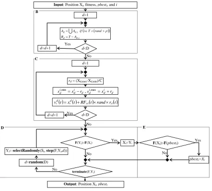
Figure 3: The schematic diagram of stochastic local search. (B) Update the list of repulsive particles, (C) Initialize of repulsion/attraction mechanism, (D) Update position module, (E) Update previous best position module.

D. Adapting Stochastic Local Search

In PSO, the new position of a particle depends on its current position, velocity vector, social and cognitive

components. It seems that if the velocity vector or the social component is too large, the PSO algorithm ignores the good solutions that are exists in nearby regions. Figure 2 shows the searching behavior of a particle driven by

x

Skipped region

f(x)

Local region

xc: Particle’s current position

xc xp xg

xp: Particle’s best solution

xg: Global best solution

xn: Particle’s next position

xn

xn: Optimal solution

No No

Yes

No Yes

Yes

No d=1

d<D d=d+1

d i d i d d i d i

d x r s x r

s,min  , ,max   rd = (Xd,max-Xd,min)/C

 

t x

 

t RF

 

t rand r

 

t y_id  _id  _id   _d

terminate(F,Yi)

Yi= selectRandomly(Si, step(F,Yi,d))

F(Yi)>F(Xi) Xi=Yi F(Xi)>F(pbesti) Yes

pbesti=Xi d=1

 

 

i d d

i d d

A T R

rand T i if A A

, ,  

  







d=d+1 d<D

B

C C

Input: Position Xi, fitness, pbesti, and i

No

D E

d=random(D)

xo

69 equation (1) in one dimensional space. It would lead the

particle to some search space and skip local region around particle. The local region around an individual may provide valuable additional information, and the local exploration enhances the particle searching ability and may gravitate it toward better position. This fact encourages us to introduce a stochastic local search into the PSO.

The flowchart of the proposed stochastic local search is presented in Figure 3. The stochastic local search acts as repulsive or attractor for each target particle. Following the Figure 3, a description of the proposed approach for repulsion or attraction mechanism is provided as follows: first, before the stochastic local search starts, the lists of particles which are contribute as attractor or repulsive in each dimension are updated; then the repulsion/attraction regions are initialized around each particle iT, and these particles fly stochastically in their local search regions to find better positions, if it is possible, as illustrated in Figure 2 and Figure 4. Each step of the stochastic local search navigates the particle to a new position. If the new position has better fitness than the previous position, the previous position is replaced by the new one. Also, the new fitness is compared with the

fitness of pbest. The new position is considered as pbest if it has the better fitness value than pbest.

E. Repulsion/Attraction Mechanism

In PSO, the inertia weight w is used to balance exploration and exploitation, but the local information about the landscape around an individual is not taken into account. Such information is valuable and encourages the particles to discover local unknown regions. Such discovery process adaptively accomplished throughout iterations.

In this paper, we proposed the concept of repulsion/attraction region to encourage the particles to escape from their positions and find better solutions in their local landscapes. A similar concept, called repulsive velocity, is proposed in ‎[29], ‎[30], ‎[31] to improve the performance of the original PSO. The proposed approach in SPSO-Lk algorithm differs from the concept of repulsive velocity vector introduced in ‎[29], ‎[30]. The repulsion/attraction mechanism is based on a dynamic decision making process that perform the stochastic local search around target particles. The concept of repulsion/attraction region is described in Figure 4.

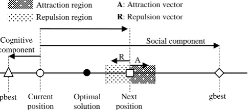
Figure 4: The repulsion/attraction region around a target particle: The repulsion vector represents displacement from the next position toward optimal solution while the attraction vector represents displacement toward global best position.

The attraction region forces the particle to drive toward the global best position, while the repulsion region encourages the particle to move in opposite direction of the global best position. The attraction and repulsion vectors respectively represent the displacement of the target particle in the attraction and repulsion regions. The repulsion region provides an enhancement in searching capability of the particles by enabling them to explore some parts of skipped regions. Also it mitigates the premature convergence of the PSO driven by (1).

The repulsion/attraction regions provide the search spaces for stochastic local search. For this purpose, during each iteration, the particles are sorted according to the value of their pbest. Then k best particles will be selected as members of set T, and a set of local regions are determined around them. As described previously, it is possible to set a static value to k or it can be set adaptively

throughout iterations. In this study we used dynamic version of k parameter. The value of k parameter dynamically adjusted based on iteration intervals, as shown in the following equation:

   

 

  

max

iter iter n n

k (11)

Where n is the number of particles in the swarm. Under this method, the number of particles which employ the local search is linearly decreased. At the first interval all of the particles are considered, while at the last interval only the global best particle is considered.

Update the list of repulsive particles: Due to SLS, it is possible for a particle to find a better position in repulsion/attraction region. Before SLS is started, a particle should be located in its repulsion or attraction region. The particle is called repulsive, if it is located in the repulsive region, otherwise it is called attractor R _A

Next position

gbest pbest

Attraction region

Repulsion region R: Repulsion vector

Current position

A: Attraction vector

Optimal solution

Social component Cognitive

particle. The repulsive particles tend to move in opposite direction of global best particle, while the attractor ones tend to move forward in direction of the global best particle. We defined a list R_d 



R_d,1,R_d,2,...,R_d,k



called repulsion list that contains the repulsive particles, as well as an attraction list A_d 



A_d,1,A_d,2,...,A_d,_p



that contains

attractor particles. More precisely, the attraction and repulsion list are defined for each dimension of the search space. The following condition should be satisfied by

repulsion and attraction lists:



n



d each for R A and R A

T d d d d  1,2,.., ,

where n represents the number of dimensions of the search space, and T is the set of particles which performs the local search. The repulsion function depends on the attractive and repulsive lists. For the particles that belong to the attraction list of dimension d, RF_id returns 1, while for the other ones return -1.









       d d id R i if A i if RF 1 1 (12)

As shown in Figure 3, before the SLS is begun, the list of repulsive or attractor particles for each dimension d

should be updated. The repulsion function updates these lists based on the predefined probability , where the

probability  is adaptively adjusted throughout iterations.

The repulsion function updates the lists as following:









i d d i d d A T R rand T i if A A , ,      



 (13)

Where Ad is the union of the candidate particles which

belong to the set T and the rand produces a value larger than threshold . The rand is a random function from the interval [0,1] drawn from a normal distribution. The other particle which are not belong to Ad constitute the

repulsive set R_d for a given dimension d.

Initialize the Repulsion/Attraction Mechanism: The local search starts by initializing the required parameters. At every iteration, after an individual i flies to its new position, if iT, it moves stochastically around its position to discover a new better position. The radius of repulsive/attractive region is decreased linearly throughout the iterations. The local search space along each dimension d of the search space for an individual i is defined as:

 

 

 

 

t x

 

t r

 

t s t r t x t s d i d i d d i d i d     max , min , (14)

Where si_d,min

 

t and s_di,max

 

t respectively represent the minimum and maximum positions of repulsion/attraction region along dimension d for stochastic local search. The radius r_d is used to control the search interval along each dimension and is defined as following:

 

 

t

C X X

t

r_d  d,max d,min  (15)

Where t is defined in (7),X_d,max and X_d,min respectively represent the maximum and minimum values of the search space along each dimension, and C is used to define the ratio of the radius against the search space. In this paper, we set r to the 5% of the solution space. The value of r_d

adaptively adjusted throughout iterations. The init function

 



init receives the n-dimensional vector r and selects the start point for the stochastic local search around candidate particles. It uses the repulsion function RF to determine if the start point should be in repulsion or attraction part of the local region. The start point in each dimension is defined as:

 

t x

 

t RF

 

t rand r

 

t

y id d

d i d

i     (16)

where rand is a random parameter from the interval [0,1] drawn from a normal distribution. Based on these formulations, the local search space will be



s if i T

S i  . Here we have not used any memory,

so we will have M

 

 .

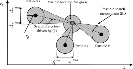
Figure 5 represents the initiation of local search space around candidate particles. The local search spaces introduce the uncertainty about the position of candidate particles, improve the balance between exploration and exploitation of the PSO, and result the better solutions for the target function. In PSO driven by (1), a particle has a hard constriction on its search trajectory, but in SPSO-Lk, see Figure 5, the search trajectory is extended to a search area. In the early iterations the algorithm tries to explore the neighbor areas, so the neighborhood radius r has the largest value. As the algorithm proceeds, the neighborhood radius is decreased and the exploitation is preferred. The triangular region in Figure 5 represents the concept of dynamic neighborhood radius.

Update Position: The SLS encourages each particle i

to explore its local region. After the start point around particle i is set to Y_i, the SLS is begun. At each step of the SLS, the drandom

 

D returns a dimension in which the next position should be determined. The function

)) , , ( , (s i i

i selectRandomly step Y d

Y   receives the local

search space si, current position Y_i, and the problem , and return the next position. A random walk approach is used to select the next position of Yi. After the particle

71 Figure 5: Local search regions associated with candidate particles.

This iterative process will continue swam by swarm until a termination criterion is satisfied. At each step, the

 



terminate function determines if the SLS should be

terminated or not. The process is terminated if the maximum number of steps is satisfied or degree of improvement is larger than predefined threshold Thimp.

Degree of improvement represents the percentage of improvement on the fitness of candidate particle.

Update Previous Best Positions (pbests): As described in previous subsection, after the position X_i is replaced with new position Y_i, if the candidate solution Y_i

is in the set S'_i

 

 of solutions of the particle i, then X_i

is used to update the previous best position (pbesti) that ever found by particle i has in the search space. If the fitness of candidate solution X_i is better that the fitness of previous best position, the previous best position is replaced by X_i. If stochastic local search returns “no-solution”, the previous best position remains unchanged.

F. UpdateGlobalBestPosition(gbest)

SPSO-Lk has two passes during every iteration. At the first pass, the global move evaluates the pbest of each individual and selects the best pbest as new gbest. The second pass is performed by the local move. The local move only evaluates the fitness of the particles which are belong to set T. If the current fitness of a particle is better than the gbest, the gbest is replaced by current position of the particle.

4.EXPERIMENT AND EVALUATION

In this section, the experiments that have been done to evaluate the performance of the proposed PSO algorithm are described. The performance of the proposed algorithm is evaluated for finding implanted motifs in a set of DNA sequences.

The SPSO-Lk is used for discovering motif in DNA sequences. In recent years many algorithms for finding

 

l,d -motif in biological sequences are proposed ‎[8]-‎[19]. However, A few applications of the PSO for motif discovery are available ‎[8], ‎[9]. Discovering the implanted motifs in DNA datasets plays important role in bioinformatics field. A DNA sequence consists of four types of nucleotide: A, C, G, T. DNA motifs which constituted from these nucleotides, are structural patterns that occur frequently in a set of nucleotide sequences. Sometimes, these motifs directly determine the functions of the sequences in which they occur.

The objective of SPSO-Lk Motif Finder is to find the

 

l,d degenerative motifs of length l that are mutated at most d symbol position of original motif. The pattern shared by these motif instances is referred to as consensus motif. Given N nucleotide sequences



s1,s2,...,s_N



, the

 

l,d -motif discovery problem is formulated as follows: assume W be a fixed but unknown sequence of nucleotides of length l, and each sequence s_i contains a variant of W with mutation at maximum d points, the algorithm should find the positions of the consensus motif in each sequence.

A. Identification of Consensus motif

The SPSO-Lk population is composed of a set of candidate consensus motifs. Each particle in the SPSO-Lk is a vector of positions of the motifs in the sequences. In other words, each particle represents a N-dimensional vector where the value of each dimension contains the position of the motif in the corresponding sequence. It is assumed that a single motif exits per sequence.

The SPSO-Lk takes a set DNA which contains N sequences of nucleotide with planted motifs of length l

with d point mutation and returns a list of candidate motif positions such that each motif should have fitness values above a certain threshold.

Initializing the population is the first issue in SPSO-Lk motif finder. As the size of the population increases, the time consumption of the algorithm increases. While taking Search trajectory

driven by (1)

Particle i Particle j

Particle k

max , 2

j

s

max , 1

i

s

x1 Possible search region using SLS

min , 1

i

s

Possible location for gbest

x2

max , 2

j

s

d

a larger amount of the subsequences occurring in the sequences as the initial population instead of ones with good fitness values increase the quality of solutions in some cases, but it will also increase the time of the algorithm to evaluate every individual of the population. So, to balance between these issues we use an informed initialization method based on Fast Motif Discovery Method ‎[9]. This method returns good motifs which can be used as an initial population.

After the initial population is created, at every iteration the SPSO-Lk select the best individual (gbest) with

highest fitness value and produces new population based on that and the previous best position of each individual (pbest). Also, at every iteration a stochastic local search

is performed around each individual to obtain better solutions. The local search is used to shift the position of the motif in a randomly selected sequence to the left or right. The motif position is updated if its new fitness is better than the previous fitness.

Another consideration is the controlling of the flying of an individual in the search space. In order to achieve these goal in the SPSO-Lk, the algorithm parameters modified as follows:

max max

max X and X V

V  UB  (17)

min min

min X and X V

V  _LB  (18)

Where the upper bound X_UB represents the largest position in the input sequences, and the lower bound X_LB

represents the smallest position in the input sequences. The proposed algorithm performs the previously described steps until the stop criteria are satisfied. Different types of criteria can be applied in optimization problem. Two different types of criteria used here. The first one is based on the fitness function, and the second one is based on iteration number. If the fitness value of the best individual is above a predefined threshold then the algorithm is stopped. If the algorithm can not obtain the threshold, then it is stopped after the certain number of iterations.

B. Fitness Function

Fitness function is one of the main considerations in optimization problem, which has an important role in success of the algorithm. In SPSO-Lk, each individual is evaluated based on a fitness function. For

 

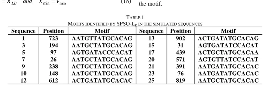
l,d -motif discovery problem a probabilistic fitness function is developed. The fitness function is based on Gibbs sampling mechanism defined in ‎[16] and ‎[17]. Based on this fitness function, the motifs which have fewer mutated position obtain greater values. Also the greater residue frequencies in the motif positions increase the fitness of the motif.

TABLE 1

MOTIFS IDENTIFIED BY SPSO-LK IN THE SIMULATED SEQUENCES

Sequence Position Motif Sequence Position Motif 1

3 5 7 9 10 12

723 194 97 26 238 148 612

AATGTTATGCACAG AATGCTATGCACAG AGTGATACCCACAT AATGCTATGCACAG ACTGCTATGCACAG AATGCTATGCACAG ACTGATATGCACAC

13 15 17 20 21 23 25

902 31 439 571 391 76 819

ACTGATATGCACAG AGTGATATCCACAT ACTGCTATGCACAA AGTGTTATCCACAT AATGATATGCACAC AATGATATGCACAC AATGCTATGCACAC

C. Experimental Results

To evaluate performance of the proposed algorithm, we performed different experiments on simulated and real DNA sequences. The first experiment is performed on the simulated sequences. For this experiment, 25 random sequences of length 1000 have been generated. Also an

 

l,d -motif with different values for l and d is planted in the sequences. For this problem, we have performed experiments to identify

 

14,4 motifs. The population

contains 100 individual. For larger values of l and d the bigger population size results better solutions. Table 1

represents the identified motifs and their positions in simulated sequences. Note, only the motifs in 14 sequences are shown.

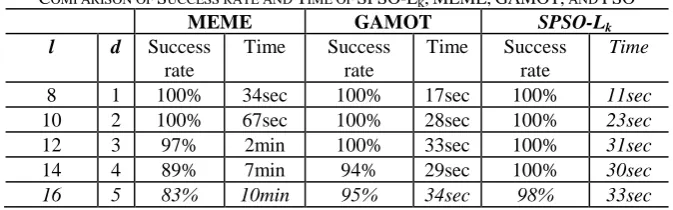
73 TABLE 2

COMPARISON OF SUCCESS RATE AND TIME OF SPSO-LK,MEME,GAMOT, AND PSO

MEME GAMOT SPSO-Lk l d Success

rate

Time Success rate

Time Success rate

Time

8 1 100% 34sec 100% 17sec 100% 11sec

10 2 100% 67sec 100% 28sec 100% 23sec

12 3 97% 2min 100% 33sec 100% 31sec

14 4 89% 7min 94% 29sec 100% 30sec

16 5 83% 10min 95% 34sec 98% 33sec

The experimental results show that the proposed algorithm outperforms MEME. Also, it relatively has a

better performance than the GAMOT algorithm.

TABLE 3

IDENTIFIED MOTIFS FOR REAL BIOLOGICAL SEQUENCES

Name Pattern MEME GAMOT SPSO-Lk

GATA CTTATC CTTATC CTTATC TTATCG CuRE TTTGCTC TTTGCTC TTTGCTC TTTGCTC BAS1 TGACTC - TGACTC TGACTC ACE2 GCTGGT GCTGGT - GCTGGT

AP1 TTANTAA - - TTAATAA

In the second experiment the SPSO-Lk is tested on a set of erythroid sequences. These sequences are tested for the GATA box which should have sequence (T/A)GATA(A/G) and its reverse complement TATC box which should have a sequence (C/T)TATC(A/T). For this problem the identified motifs in the sequences are TTATCA, CGGTCA, CTATCA, AGATAA, TGGTAC, CTATCT, TGGTCA, TTGTAA, TTATCT, TTATCC, AGATAT, AGATAT, CTGTAT, and TTATCT.

For the third experiment, we used the real biological sequences from the SCPD dataset ‎[19]. SCPD is a dataset of different transcription factors for yeast. We have evaluated the performance of SPSO-Lk against MEME, and GAMOT algorithms. The motifs identified by the proposed method are shown in Table 3. As shown in Table 3, all of the methods successfully discover the implanted motif in GATA and CuRE sequences. The MEME algorithm fails for finding the implanted motif for BASE1 and API sequences. Also, the GAMOT algorithm fails for finding motifs in ACE2 and API. The SPLSO successfully discovers the implanted motifs in each sequence. In SPSO-Lk algorithm, the stochastic local search acts as a sliding window on the nucleotide sequences. So, the algorithm can observe the nearby regions to find better positions. The above experiments demonstrate the effectiveness of the SPSO-Lk algorithm for

 

l,d -motif discovery problem.

5.CONCLUSIONS

In this work we present a combinatorial optimization based on improved version of PSO and Stochastic local search employing an intelligent inertia weight to significantly improve the performance of the original PSO. The use of local exploration seems to provide a good balance between exploitation and exploration of the PSO algorithm. The local landscape around each particle allow us to test many other local search methods such as tabu search and simulated annealing as well as other random walk techniques.

In the original PSO, the individuals are gravitated rapidly toward the global best particle and the population rapidly converges to a point around the best particle. The high speed convergence may occur due to constriction on the particles trajectories and the premature convergence. By considering local landscape associated with each individual as a function of time, the stochastic local search method provides an efficient exploration that helps the population to avoid premature convergence. Also, a local exploration relaxes the hard constriction on the particle trajectory and provides the required diversity for the particle trajectory.

6.REFERENCES

[1] M.-F. Sagot. "Spelling approximate repeated or common motifs using a suffix tree", In C. L. Lucchesi and A. V. Moura, editors, LATIN’98: Theoretical Informatics, Lecture Notes in Computer Science, pp. 111–127. Springer-Verlag, 1998.

[2] G. Pavesi, G. Mauri, G. Pesole, "An algorithm for finding signals of unknown length in DNA sequences", Bioinformatics;17 Suppl 1:S207-14, 2001.

[3] E. Eskin, U. Keich, M. S. Gelfand, P. A. Pevzner. “Genome-Wide Analysis of Bacterial Promoter Regions.” In Proc. of the Pacific Symposium on Biocomputing (PSB-2003). Kaua’i, Hawaii: January 3-7, 2003.

[4] G. Z. Hertz, and G. D. Stormo, “Identifying DNA and protein patterns with statistically significant alignments of multiple sequences”, Bioinformatics. 15(7-8):563-77,1999.

[5] T. L. Bailey, and C. Elkan, "The value of prior knowledge in discovering motifs with MEME", Proc. Int. Conf. Intell. Syst. Mol. Biol., 3, 21–29, 1995.

[6] C. E. Rouchka, \A brief overview of Gibbs sampling." [online]

Available:http://kbrin.a-bldg.louisville.edu/rouchka/HOMEPAGE/PAPERS/gibbs.pdf. [7] N. Karaoglu, S. M. Stroh, and B. Manderick, "GAMOT: An

Efficient Genetic Algorithm for Finding Challenging Motifs in DNA Sequences", In Proc. of Trim Siz, 2006.

[8] C. T. Hardin, E. C. Rouchka, “DNA motif detection using particle swarm optimization and expectation-maximization”, In IEEE Proc. of Swarm Intelligence Symposium, SIS, pp. 181- 184, 2005. [9] U. Keich and P. Pevzner. Finding motifs in the twilight zone. In

Proceedings of the Sixth Annual International Conference on Research in Computational Molecular Biology, RECOMB, pages 195–204, 2002.

[10] E. Rocke and M. Tompa. An algorithm for finding novel gapped motifs in DNA sequences. In Sorin Istrail, Pavel Pevzner, and Michael Waterman, editors, Proceedings of the 2nd Annual International Conference on Computational Molecular Biology (RECOMB-98), pages 228–233, New York, 1998. ACM Press. [11] L. Yang, E. Huang, and V.B. Bajic. Some implementation issues of

heuristic methods for motif extraction from dna sequences. Int.J.Comp.Syst.Signals (To Appear), 2004.

[12] M.-F. Sagot. "Spelling approximate repeated or common motifs using a suffix tree", In C. L. Lucchesi and A. V. Moura, editors, LATIN’98: Theoretical Informatics, Lecture Notes in Computer Science, pp. 111–127. Springer-Verlag, 1998.

[13] G. Pavesi, G. Mauri, G. Pesole, "An algorithm for finding signals of unknown length in DNA sequences", Bioinformatics;17 Suppl 1:S207-14, 2001.

[14] E. Eskin, U. Keich, M. S. Gelfand, P. A. Pevzner. “Genome-Wide Analysis of Bacterial Promoter Regions.” In Proc. of the Pacific Symposium on Biocomputing (PSB-2003). Kaua’i, Hawaii: January 3-7, 2003.

[15] G. Z. Hertz, and G. D. Stormo, “Identifying DNA and protein patterns with statistically significant alignments of multiple sequences”, Bioinformatics. 15(7-8):563-77, 1999.

[16] T. L. Bailey, and C. Elkan, "The value of prior knowledge in discovering motifs with MEME", In Proceeding of International Conference on Intelligent Systems and Molecular Biology, Vol. 3, pp. 21–29, 1995.

[17] X. Wu, J. Cheng, C. Song, and B. Wang. A combined model and a varied gibbs sampling algorithm used for motif discovery. In Yi-Ping Phoebe Chen, editor, 2nd Asia-Pacific Bioinformatics Conference, volume 29 of CRPIT, pp. 99-104, Dunedin, New Zealand, 2004. ACS.

[18] N. Karaoglu, S. M. Stroh, and B. Manderick, "GAMOT: An Efficient Genetic Algorithm for Finding Challenging Motifs in DNA Sequences", In Proc. of Trim Siz, 2006.

[19] J. Zhu and M. Zhang. “SCPD: a promoter database of the yeast Saccharomyces cerevisiae”, Bioinformatics 15:563-577, 1999. [20] J. Kennedy and R. Eberhart, "Particle swarm optimization", in

Proc. IEEE Int. Conf. Neural Networks, vol. 4, 1995, pp. 1942– 1947.

[21] B. C. H. Chang, A. Ratnaweera, and S. K. Halgamuge, "Particle Swarm Optimization for Protein Motif Discovery", In journal of Genetic Programming and Evolvable Machines, Vol. 5, pp. 203– 214, 2004.

[22] C. T. Hardin, E. C. Rouchka, “DNA motif detection using particle swarm optimization and expectation-maximization”, In IEEE Proc. of Swarm Intelligence Symposium, SIS, pp. 181- 184, 2005. [23] Y. Shi and R. C. Eberhart, “Parameter selection in particle swarm

optimization,” in Proc. Evolutionary Programming VII, vol. 1447, 1998, pp. 591–600.

[24] H. Hoos, and T. Stützle, “Stochastic Local Search: Foundations and Applications”, Morgan Kaufmann Publishers, San Francisco, CA, USA. 2004.

[25] R. Akbari, K. Ziarati, “Combination of Particle Swarm Optimization and Stochastic Local Search for Multimodal Function Optimization”, In proceeding of IEEE Pacific-Asia Workshop on Computational Intelligence and Industrial Application, pp. 388-392, 2008.

[26] M. O. Rayes, V. Trevisan, “Factorization of Chebyshev Polynomials”, 1998.

[27] A. Ratnaweera, S. K. Halgamuge, and H. C. Watson, “Self-Organizing Hierarchical Particle Swarm Optimizer With Time-Varying Acceleration Coefficients”, In IEEE Transactions on Evolutionary Computation, Vol. 8, No. 3, pp. 240-255, 2004. [28] Chia-Nan Ko a,*, Ying-Pin Chang b, Chia-Ju Wu, “An

orthogonal-array-based particle swarm optimizer with nonlinear time-varying evolution”, Applied Mathematics and Computation 191 (2007) 272–279.

[29] J. Riget, and J. S. Vesterstrom, “A Diversity-guided Particle Swarm Optimizer-The ARPSO EVALife”, Tech. Rep. 2002-02.

[30] S. T. Hsieh, T. Y. Sun, C. L. Lin, and C. C. Liu, “Effective Learning Rate Adjustment of Blind Source Separation Based on an Improved Particle Swarm Optimizer”, In IEEE Transactions on Evolutionary Computation, Vol. ,No. , pp. , 2007.

[31] J. H. Seo1, C. H. Im, C. G. Heo, J. K. Kim, H. K. Jung, and C. G. Lee. “Multimodal Function Optimization Based on Particle Swarm Optimization”, In IEEE Transaction on Magnetics, Vol. 42, No. 4, pp. 1095-1098, 2006.