Numerical solution of higher index DAEs using their IAE's structure: Trajectory-prescribed path control problem and simple pendulum

(1)

University of Mazandaran, Iran http://cjms.journals.umz.ac.ir ISSN: 1735-0611 CJMS.7(1)(2018), 1-15

Numerical solution of higher index DAEs using their IAE’s structure: Trajectory-prescribed path control

problem and simple pendulum

G. Karamali1 and B. Shiri2

1,2 _{PhD, Shahid Sattari Aeronautical University of Science and} Technology, South Mehrabad, Tehran, Iran.

Abstract. In this paper, we solve higher index differential braic equations (DAEs) by transforming them into integral alge-braic equations (IAEs). We apply collocation methods on continu-ous piecewise polynomials space to solve the obtained higher index IAEs. The efficiency of the given method is improved by using a recursive formula for computing the integral part. Finally, we apply the obtained algorithm to solve a trajectory-prescribed path control problem and a model of simple pendulum. The numerical experi-ments show efficiency of the given techniques.

Keywords: Diﬀerential algebraic equations, integral algebraic equations, trajectory-prescribed path control problem, simple pen-dulum, continuous piecewise collocation methods.

2000 Mathematics subject classification: 65L80, 65R20, 45L05.

1. Introduction

For almost half a century, diﬀerential algebraic equations (DAEs) have been studied and used for modeling of complicated technical processes [2, 4, 10, 12, 16]. Most numerical methods for DAEs are based on standard methods of the ordinary diﬀerential equations (ODEs) [4, 10]. It is well known that the robust and numerically stable application on these ODE

1_{Corresponding author: g [email protected]} Received: 17 October 2015

Revised: 8 January 2017 Accepted: 2 February 2017

(2)

methods for higher index DAEs (index greater than 1) have to be based on the structure of DAEs ([4]). Roughly speaking, the index (diﬀerential index), is the minimum number of diﬀerentiations needed to transform the DAE system into an ODE system. The higher the index is, the higher the numerical problems we get.

Motivated by physical examples, in this paper we solve the DAEs of the form

Ax′(t) =F(t, x(t)), (1.1) where A ∈ L(Rr, Rr) is a nonsingular matrix with constant rank and

F ∈C(I×Rr_{, R}r₎_._{The idea behind the method we introduce, is easy.}

We integrate the equation (1.1) and we obtain an integral algebraic equation (IAE) and then we solve it numerically. However it needs some consideration to operate eﬃciently that we will discuss in the next section.

A system of Voltera integral equations of the form

A(t)y(t) + ∫ t

0

κ(t, s, y(s))ds=f(t), t∈I := [0, T], (1.2)

where A ∈ C(I, Rr×r₎_{, f} _∈ _C₍_{I, R}r₎_, _and _κ _∈ _C₍_D_×_Rr_{, R}r₎_, _with

D:={(t, s) : 0≤s≤t≤T} is an IAE ifA(t) be a singular matrix with constant rank on I = [0, T]. In recent decades, IAEs have got popular and have been studied by researchers ([6, 9, 7, 17, 18, 15]). Numeri-cal solutions of higher index IAEs of Hessenberg type using collocation methods on piecewise polynomials space are studied in [17, 18]. It is well-known that by increasing the index of DAEs, the order of the nu-merical methods decreases. We can choose an appropriate method of higher order to prevent these reductions, by applying the collocation methods on piecewise polynomials space. Therefore, in this paper, we use these methods to obtain eﬃcient algorithm for solving higher index. One of the interesting applied model in physics is a model of simple pendulum which leads to DAEs of the form (1.1). The equation of motion of a point mass m suspended from a massless rod of length l

under the inﬂuence of gravity g is

d2θ dt2 +

g

lsin(θ) = 0 (1.3)

(3)

The next problem that we investigate in this paper, is a trajectory-prescribed path control (TPPC) problem [3, 4]. This problem was in-troduced in [3]. We consider a space shuttle, returning from its mission which has to reenter the atmosphere. In the simulation of space shuttle, the shape of the trajectory is often prescribed by appending a set of path constraints to the equations of motion. The model equation then become a nonlinear semi-explicit DAE system.

The next sections are organized as follows: In section 2, we recall implementation of the continuous piecewise collocation methods from [6] for IAEs. In section 3,we show how we can apply these methods for DAEs. Finally, in section 4,we report numerical examples of the selected problems to show the eﬀectiveness and eﬃciency of the methods.

2. Preliminaries

The collocation methods on the piecewise polynomials spaces are very suitable for the equations with integral or diﬀerential operators. They have easily implementable strategy, rapid convergent properties, less computational cost, and good stablity properties. Especially in solving many operator equations, their convergence orders don’t change when the integrals are discretized (See [6, 17, 18]). Let

Ih:={tn: 0 =t0 < t1 < ... < tN =T}

be a given (not necessarily uniform) partition ofI,and setσn:= (tn, tn+1], σn := [tn, tn+1], with hn = tn+1−tn, n= 0,1, ..., N −1 and diameter

h = max{hn : 0 ≤ n ≤ N}. Each component of the solution of (1.2)

(the vector functiony(t)) is approximated by elements of the piecewise polynomial space

S(0)

m (Ih) :={v∈C(I) :v|σn ∈πm(n= 0,1, ..., N −1)}, (2.1)

where πm denotes the space of all (real valued) polynomials of degree

not exceeding m and v|σn is the restriction of function v to closure of σn. The collocation solutionuh∈

( S(0)

m (Ih) )r

for (1.2) is deﬁned by the equation

A(t)uh(t) + ∫ t

0

k(t, s, uh(s))ds=f(t), (2.2)

for t ∈ Xh = {tn,i := tn+cihn : 0 = c0 < c1 < . . . < cm ≤ 1, n =

0,· · · , N −1} and the continuity conditions

(4)

The collocation parameterscicompletely determine the set of collocation

pointsXh. By deﬁningun=uh|σn ∈(πm)

r_,_{we have}

un(tn+shn) = m ∑

j=0

Lj(s)Un,j, s∈(0,1], (2.4)

Un,i:=u(tn,i),

where the polynomials

Lj(v) := m ∏

k=0

k̸=j

v−ck

cj−ck

, j = 0, . . . , m

denote the Lagrange fundamental polynomials with respect to the dis-tinct collocation parametersci. By partitioning the domain of integral

in (2.2) and changing of variables, we have

A(tn,i)Un,i+Fn,i+h ∫ ci

0

κ(tn,i, tn+shn, L0(s)Un−1(tn)

+

m ∑

j=1

Lj(s)Un,j)ds=f(tn,i),

(2.5)

fori= 1, . . . , m, where the lag terms are deﬁned by

Fn,i=h n_∑−1

l=0

∫ 1

0

κ(tn,i, tl+shl, L0(s)Ul−1(tn) + m ∑

j=1

Lj(s)Ul,j). (2.6)

By solving the system (2.5), approximate solution of (1.2) is deter-mined at the collocation points and attn+1 by

un(tn+1) =L0(1)un−1(tn) + m ∑

j=1

Lj(1)un(tn,j).

Remark 2.1. A suitable method to solve the system (2.5) is Newton’s iterative method, since it can be proved (see [1]) that this method con-verges to the solution Un,i by the initial guess un−1(tn) for suﬃciently

small h. Therefore, in the prescribed method we use the initial guess [_|un−1(tn), . . . , u_{z n−1(tn_})

m times

].

(5)

the order of the quadrature rule would be at least in the same order of the method (O(hm+1)),

∫ ci

0

k(tn,i,tn+shn, L0(s)Un−1(tn) + m ∑

j=1

Lj(s)Un,j)ds

≃

m ∑

j=1

ai,jk(tn,i, tn+cjhn, Un,j),

∫ 1

0

k(tn,i,tl+shl, L0(s)Ul−1(tn) + m ∑

j=1

Lj(s)Ul,j)ds

≃

m ∑

j=1

bjk(tn,i, tn+cjhn, Ul,j),

with ai,j = ∫ci

0 Lj(t)dt and bj =

∫1

0 Lj(t)dt. Using this quadrature rule simpliﬁes our computations considerably. If all of the integrals are com-puted by quadrature rule then the method is called fully discretised continuous colocation method (DCCM).

Remark 2.2. By choosing cm = 1, for m ≥ 2, we have tn+1 = tn,m

and u(tn+1) =u(tn,m), thus we obtain un+1 = Un,m from the previous

subinterval without reusing (2.4).

3. The continuous piecewise collocation methods for DAEs

To the DAEs of the form (1.1), by integrating we obtain

Ax(t)− ∫ t

0

F(s, x(s))ds=Ax(0), (3.1)

which is an IAEs of the form (1.2) and hence one can use the numerical methods of the pervious section to solve this equation. Considering the kernel of this equation which is independent of t, we can restate the equations of lag terms in such a way that the computational cost decreases considerably. In this case the lag terms are computed as

Fn,i=h n−1

∑

l=0

m ∑

j=0

bjF(tl+cjhn, Ul,j), (3.2)

wherem is a ﬁxed integer depend on the method (usually we choose m

(6)

because of the presence of tn,i for each n and i. But for DAEs, we can

use the recursive formula

Fn+1,i=Fn,i+ m ∑

j=0

bjF(tn,j, Un,j)

to obtain Fn,i which is independent of i, (and we can drop index i).

Thus the computation will be of orderO(n),which makes this method compatible with the Runge-Kutta methods.

Therefore, for the DAEs (1.1), the method can be simpliﬁed to

F0 =A(t0)y0, U0,0 =y0,

A(tn,i)Un,i=Fn+h m ∑

j=0

aijF(tn,j, Un,j), i= 1, . . . , m

Fn+1 =Fn+h m ∑

j=0

bjF(tn,j, Un,j),

Un+1,0:=un(tn+1) =

m ∑

j=0

Lj(1)Un,j,

(3.3)

forn= 1, . . . , N −1,and h= _NT.

Remark 3.1. Note that, these methods are of Runge-Kutta type iﬀ

Un+1 = Fn+1. This condition holds for the case cm = 1, for m ≥ 2,

which has considerable simpliﬁcation in the formula (3.3). In this case,

Un+1=Fn+1=Un,m.

The restrictions exist in choosingcis for the ﬁrst IAEs of Hessenberg

type [17]. Due to [17], we should choose ci such that c0= 0 and ϱ= max{|λ1|,|λ2|} ≤1,

whereλ1 andλ2 are eigenvalues of the stability matrix Ae−1B.The ma-trices Ae−1 and B are introduced in [17] as follow

e

A=     

1 0 . . . 0

a10 a11 . . . a11 ..

. ... . .. ...

am0 am1 . . . amm     

and

B =     

L0(1) . . . Lm(1)

am0−b0 . . . amm−bm

..

. . .. ...

(7)

These eigenvalues can be computed as follow

λ1= 1 2

(

tr(Ae−1B) + √

(tr(Ae−1_B₎₎2−₄₍_L 0(1))2

)

, (3.4)

λ2= 1 2

(

tr(Ae−1B)− √

(tr(Ae−1_B₎₎2₋₄₍_L 0(1))2

)

, (3.5)

tr(Ae−1B) =L0(1)

( 2 + m ∑ i=1 1 ci + m ∑ i=1 1 1−ci

)

, (3.6)

forcm<1 and

λ1 = 0, (3.7)

λ2= (−1)m

m_∏−1

i=1 1−ci

ci

, (3.8)

forcm = 1 (see [17]). Since the solution obtained from (3.3) is exactly

the same solution obtained from (3.1), by applying (DCCM), the con-vergence results of [17] also hold for (3.3). Therefore, the order of the method decreases by increasing the index of the DAEs and for higher index DAEs, we should use higher order methods which can be achieved by increasingm.

4. Sample problems

In this section, we use some selected sample problems to illustrate the eﬀectiveness and high accuracy of the given method.

. 6 -@ @ @ @ @ @x r l x1 x2

?_F_gm₌_mg

F

?Fx2

F

Fx1

Figure 1. Simple pendulum-scheme

4.1. Simple pendulum. In this section we consider the simple pen-dulum of length l, mass m under the inﬂuence of gravity Fg = −mg,

(8)

Table 1. Numerical results of index 3 DAE (4.1) for x1(t) withN = 500.

t method 1 method 2 ode15s

2 0.791415503888909 0.791415099102267 0.79141509926 4 −0.584175128656931 −0.584197053914579 −0.58419714676 6 −0.999568975065766 −0.999569743078752 −0.99956974661 8 −0.915348262923567 −0.915330990754696 −0.91533091583 10 0.296123754641507 0.296271070783072 0.29627172089

Computing time 2.06s 3.14s 3.76s

2 −0.611278553797112 −0.611279102303482 −0.61127910209 4 −0.811627593357415 −0.811611854396871 −0.81161178758 6 −0.029358053740116 −0.029331360716471 −0.02933124145 8 −0.402663087278485 −0.402702343380354 −0.40270251353 10 −0.955149523562636 −0.955103896242212 −0.95510369463

2 0.791415170748194 0.791415099376876 0.79141509926 4 −0.584196752919579 −0.584197220670537 −0.58419714676 6 −0.999569736371046 −0.999569755689938 −0.99956974661 8 −0.915331234981749 −0.915330861481158 −0.91533091583 10 0.296269503434385 0.296272220867141 0.29627172089

[x, y]T _{and the velocity vector [}_x

3, x4]T = [ ˙x,y˙]T,one obtain the follow-ing index 3DAE problem

˙

x1=x3, ˙

x2=x4, ˙

x3=−x1λ, ˙

x4=−g−x2λ, 0 =x2₁+x2₂−l2,

(9)

2 −0.611279003691347 −0.611279108658166 −0.61127910209 4 −0.811612064882334 −0.811611737838670 −0.81161178758 6 −0.029331555088146 −0.029331165734774 −0.02933124145 8 −0.402701741692676 −0.402702663299050 −0.40270251353 10 −0.955104342069682 −0.955103550550979 −0.95510369463

2 0.791415239425474 0.791415065252080 0.79141509926 4 −0.584206187091868 −0.584196780385478 −0.58419714676 6 −0.999571288011394 −0.999569533743246 −0.99956974661 8 −0.915318931747990 −0.915331688232221 −0.91533091583 10 0.296463994504867 0.296250795527552 0.29627172089

2 −0.611278141437346 −0.611279176060579 −0.61127910209 4 −0.811606367517056 −0.811611944121050 −0.81161178758 6 −0.029307506124896 −0.029333223880495 −0.02933124145 8 −0.402723355480016 −0.402701610197581 −0.40270251353 10 −0.955045825877874 −0.955109908908153 −0.95510369463

which is equivalent to (1.3) with some consideration. Diﬀerentiating from the last equation of system (4.1), we obtain the index 2 DAE

˙

x1 =x3, ˙

x2 =x4, ˙

x3 =−x1λ, ˙

x4 =−g−x2λ, 0 =x1x3+x2x4,

(10)

and another diﬀerentiating from the last equation of system (4.2), we can obtain an index 1 DAE

˙

x1 =x3, ˙

x2 =x4, ˙

x3 =−x1λ, ˙

x4 =−g−x2λ,

0 =x2₃+x2₄−gx2−l2λ.

(4.3)

This is called the index reduction procedure. After this index reduc-tion one can solve the index 1 DAE (4.3) by available software and codes like “ode15s” in MATLAB. However, this index reduction cannot be obtained for many DAEs because of their nonlinearity or complex-ity (sometimes the obtained equations are very complicated with many nonlinear long terms). Consequently, we are interested in direct solving of index 3 DAE (4.1). Thus, we solve all of the equations (4.1)-(4.3) as a test problem and compare them with the numerical solution of applying “ode15s” on (4.3).

Example 4.1. We consider the system (4.1)-(4.3) by the parameter

l= 1 and the consistency initial conditions

x1(0) = 1, x2(0) = 0, x3(0) = 0, x4(0) = 0, λ(0) = 0.

We use the following methods to get numerical solutions of this example on t∈[0,10] and h= 10_N withN = 500.

Method 1:: Let c = [0,0.5,0.8,0.88]. For this c, we have λ1 = −0.0016 andλ2 =−0.7389.

Method 2:: Letc= [0,0.5,0.8,0.88,1].For thisc,we haveλ1 = 0 and λ2=−0.034.

In Tables 1 and 2, we compared the obtained results with the numerical results of the command “ode15s” in MATLAB software. We set the ex-treme ode options abstol = 100epsand reltol = 100epsfor the command “ode15s”. These Tables show the eﬃciency of the method.

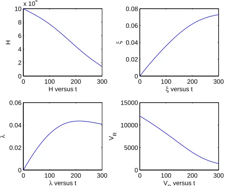
4.2. Trajectory-prescribed path control problem. Trajectory- pre-scribed path control problem for shuttle reentry was solved for diﬀerent shuttles and diﬀerent conditions (see for examples [3, 5, 19]). Here, we use the scale and data of [5]. Suppose a space shuttle with mass

m = 2.890532728 slugs, cross sectional reference area S = 1 ft2, and with relative velocityVR= 12000 ft/s,at the altitude ofH = 100000 ft,

(11)

0 100 200 300 0

2 4 6 8 10x 10

4

H

H versus t

0 100 200 300

0 0.02 0.04 0.06 0.08

ξ

ξ versus t

0 100 200 300

0 0.02 0.04 0.06

λ

λ versus t

0 100 200 300

0 5000 10000 15000

VR

V_R versus t

Figure 2. Numerical solution of TPPC problem using

method 1, withN = 250,state variables.

0 100 200 300

−10 −8 −6 −4 −2 0

γ

γ versus t

0 100 200 300

0 50 100 150

A

A versus t

0 100 200 300

2 4 6 8

α

α versus t

0 100 200 300

−20 0 20 40 60

β

β versus t

Figure 3. Numerical solution of TPPC problem using

method 1, withN = 250,state and control variables.

Here, the aerodynamic lift and drag force are given by L = 1₂ρV_R2SCL,

and D = 1₂ρV_R2SCD, respectively, where, ρ(H) = 0.002378e−H/23800,

(12)

Table 7. Numerical results of index 2 DAE (4.4)-(4.5)

att= 300 with N = 250.

method 1 method 2 method 3

H 14200.786553704 14200.786553653 14200.786553654

ϵ 0.0727991723743 0.0727991723742 0.0727991723742

λ 0.0406923062717 0.0406923062717 0.0406923062717

VR 1433.2929482465 1433.2929482436 1433.2929482436

γ −0.174532925199 −0.174532925199 −0.174532925199

A 2.3561944901923 2.3561944901923 2.3561944901923

α 7.1564690302731 7.1564690301584 7.1564690301516

β 0.4603119285387 0.4603119285335 0.4603119285300

Computing time 1.5s 2.6s 30s

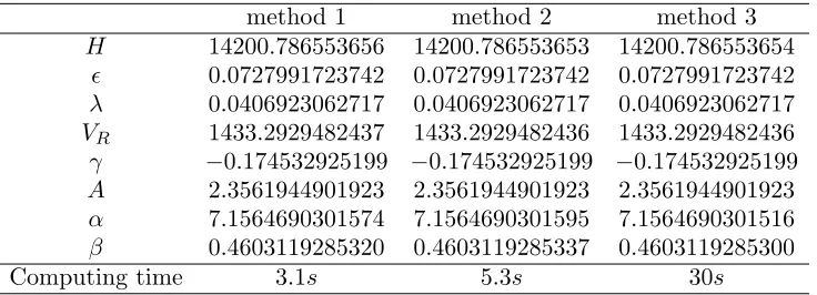
Table 8. Numerical results of index 2 DAE (4.4)-(4.5)

att= 300 with N = 500.

method 1 method 2 method 3

H 14200.786553656 14200.786553653 14200.786553654

ϵ 0.0727991723742 0.0727991723742 0.0727991723742

λ 0.0406923062717 0.0406923062717 0.0406923062717

VR 1433.2929482437 1433.2929482436 1433.2929482436

γ −0.174532925199 −0.174532925199 −0.174532925199

A 2.3561944901923 2.3561944901923 2.3561944901923

α 7.1564690301574 7.1564690301595 7.1564690301516

β 0.4603119285320 0.4603119285337 0.4603119285300

Computing time 3.1s 5.3s 30s

0.04 + 0.1C_L2,respectively. The gravity force is mg, where the gravita-tional acceleration g is given byg= _rµ2.Hereµ= 1.407653916×1016,is

the gravitational constant, r = H+ae, is the distance of shuttle from

the center of the earth, andae= 20902900,is the earth radius. The

(13)

of ﬁrst order diﬀerential equations:

H′ = VRsin(γ),

ϵ′ = VRcos(γ) sin(A)

rcos(λ) ,

λ′ = VR

r cos(γ) cos(A), V_R′ = −D

m −gsin(γ) (4.4)

−Ω2rcos(λ) (sin(λ) cos(A) cos(γ)−cos(λ) sin(γ)),

γ′ = Lcos(β)

mVR

+cos(γ)

VR (

V_R2 r −g

)

+ 2Ω cos(λ) sin(A),

+Ω

2_r_cos(_λ₎ VR

(sin(λ) cos(A) cos(γ)−cos(λ) sin(γ)),

A′ = Lsin(β)

mVRcos(γ)

+VR

r cos(γ) sin(A) tan(λ),

−2Ω (cos(λ) cos(A) tan(γ)−sin(λ)),

+Ω

2_r_cos(_λ_{) sin(}_λ_{) sin(}_A₎ VRcos(γ)

.

Here, the control parameters areαand β which show the angle and the bank of the attack, respectively. The constraints for the trajectory to be followed by the vehicle are given only in terms of zenith angleγ,and azimuth angle A:

γ = −1−9 (

t

300 )2

,

(4.5)

A = 45 + 90

(

t

300 )2

.

The system (4.4)-(4.5) is a 8 dimensional nonlinear DAE of index2. Sub-stituting the derivative of (4.5) into the last equations of (4.4), we can obtain algebraic equations forα,and β.Fort= 0,the solution of these equations gives initial conditions α0 = 2.6733 andβ0 =−0.0520.

Example 4.2. Now, we can apply the (3.3) to the DAE (4.4)-(4.5). To obtain more accurate results, we can increase m, the number of collo-cation points or increase N. For this index 2 problem, we can obtain the methods with order of convergenceO(_NT)m+1−2,[17]. Therefore, we choose

(14)

and setN = 1000 to get a more accurate result. We apply the method 1 and 2, of Example 4.1. Figures 2 and 3 illustrate the numerical solutions using method 1, with N = 250. Tables 7 and 8 show the numerical solutions of Methods 1, 2 at the end point t = 300 for N = 250,500. These tables show eﬃciency and eﬀectiveness of the introduced methods.

conclusion

In this paper we used continuous piecewise collocation methods for solving DAEs appeared in some physical models. The equations that we dealt with did not have closed form analytical solutions. Our nu-merical experiments show eﬃciency and eﬀectiveness of the proposed methods with rapid convergence, easily implementable properties, and less computational cost.

References

[1] K. Atkinson and W. Han, Theoretical numerical analysis, (Vol. 39), Berlin: Springer, 2005.

[2] U. M. Ascher and L. R. Petzold, Computer methods for ordinary differen-tial equations and differendifferen-tial-algebraic equations, (Vol. 61), SIAM, 1998. [3] K. E. Brenan, Stability and convergence of difference approximations for higher index differential algebraic systems with applications in trajectory control, PhD diss., 1983.

[4] K. E. Brenan, S. L. Campbell and L. R. Petzold Numerical solution of initial-value problems in diﬀerential-algebraic equations, (Vol. 14). SIAM, 1996.

[5] K. E. Brenan and L. R. Petzold, The Numerical Solution of Higher Iindex Diﬀerential/Algebraic Equations by Implicit Methods, SIAM J. Numer. Anal.,26(4)(1989), 976-996.

[6] H. Brunner, Collocation methods for Volterra integral and related func-tional diﬀerential equations, (Vol. 15), Cambridge University Press, 2004. [7] O. G. S. Budnikova and M. V. Bulatov, Numerical solution of integral-algebraic equations for multistep methods, Comput. Math. Math. Phys.,

52(5)(2012), 691-701.

[8] E. Eich-Soellner and C. F¨uhrer, Numerical methods in multibody dynam-ics, (Vol. 45), Stuttgart: Teubner, 1998.

[9] C. W. Gear, Diﬀerential algebraic equations, indices, and integral algebraic equations,SIAM J. Numer. Anal., 27(6)(1990), 1527-1534.

[10] E. Hairer, C. Lubich and M. Roche, The numerical solution of diﬀerential-algebraic systems by Runge-Kutta methods, Springer, 1989.

[11] E. Hairer and G. Wanner, Solving ordinary differential equations ii: Stiff and differential-algebraic problems second revised edition with 137 figures, Springer series in computational mathematics, 14, 1996.

[12] P. Kunkel and V. L. Mehrmann, Diﬀerential-algebraic equations: analysis and numerical solution, Eur. Math. Soc., 2006.

(15)

[14] K. Ochs, A comprehensive analytical solution of the nonlinear pendulum,

Eur. J. Phys., 32(2)(2011), 479.

[15] S. Pishbin, Optimal convergence results of piecewise polynomial colloca-tion solucolloca-tions for integralalgebraic equacolloca-tions of index-3,J. Comput. Appl. Math.,279(2015), 209-224.

[16] P. J. Rabier and W. C. Rheinboldt, Theoretical and numerical analysis of diﬀerential-algebraic equations,Handbook of numerical analysis, 8(2002), 183-540.

[17] B. Shiri, S. Shahmorad and G. Hojjati, Convergence analysis of piece-wise continuous collocation methods for higher index integral algebraic equations of the Hessenberg type,Int. J. Appl. Math. Comput. Sci,

23(2)(2013), 341-355.

[18] B. Shiri, Numerical solution of higher index nonlinear integral algebraic equations of Hessenberg type using discontinuous collocation methods,

Math. Model. anal.,19(1)(2014), 99-117.