DISCUSSION PAPER SERIES
DP11897
THE PEACE DIVIDEND OF DISTANCE:
VIOLENCE AS INTERACTION ACROSS
SPACE
Hannes Mueller, Dominic Rohner and David
Schönholzer
ISSN 0265-8003
THE PEACE DIVIDEND OF DISTANCE: VIOLENCE AS
INTERACTION ACROSS SPACE
Hannes Mueller, Dominic Rohner and David Schönholzer
Discussion Paper DP11897
Published 10 March 2017
Submitted 10 March 2017
Centre for Economic Policy Research
33 Great Sutton Street, London EC1V 0DX, UK
Tel: +44 (0)20 7183 8801
www.cepr.org
This Discussion Paper is issued under the auspices of the Centre’s research programme
in DEVELOPMENT ECONOMICS and PUBLIC ECONOMICS. Any opinions expressed here
are those of the author(s) and not those of the Centre for Economic Policy Research. Research
disseminated by CEPR may include views on policy, but the Centre itself takes no institutional
policy positions.
The Centre for Economic Policy Research was established in 1983 as an educational charity,
to promote independent analysis and public discussion of open economies and the relations
among them. It is pluralist and non-partisan, bringing economic research to bear on the analysis
of medium- and long-run policy questions.
These Discussion Papers often represent preliminary or incomplete work, circulated to
encourage discussion and comment. Citation and use of such a paper should take account of
its provisional character.
THE PEACE DIVIDEND OF DISTANCE: VIOLENCE AS
INTERACTION ACROSS SPACE
Abstract
More distant targets are harder to attack, and hence increased distance between potential
attackers and potential targets may drive down the death toll of conflict. To investigate this, the
current paper studies violence as interaction across space, i.e. it separates the origin from the
target of attacks. We show that a game-theoretic model based on the idea that distance matters
can deliver new insights into understanding the causes, the extent and the distribution of
violence. Key factors are the transport costs of violence and the distribution of the groups
across locations. To estimate the structural parameters of the model, we use very fine-grained
data from Northern Ireland on religious composition at each location, and on the identity of
attackers and victims in violent events from 1969 to 2001. Using these estimates we show that
more than half of the attacks in Northern Ireland were conducted across administrative ward
boundaries and that changes in the settlement patterns of the population from the 1970s to the
1980s could be responsible for a large reduction in violence. We find that both the origin and
path of attacks can be predicted with our model and that the construction of barriers by the UK
government follows these predictions.
JEL Classification: D74, K42, N44, Z10
Keywords: conflict, Ethnic Violence, Religious Violence, Spatial Data, Distance Costs,
Polarization, Segregation, Northern Ireland, Insurgency
Hannes Mueller - [email protected]
Institut d'Analisi Economica (CSIC), Barcelona GSE and CEPR
Dominic Rohner - [email protected]
University of Lausanne and CEPR
David Schönholzer - [email protected]
UC Berkeley
Acknowledgements
Acknowledgements: We thank Quentin Gallea, Yihuan Hu, Dong Ook Eun, Augustin Tapsoba and Nghia-Piotr Trong Le for excellent research assistance, and Joan Maria Esteban, Mathias Thoenig, and Debraj Ray for very useful comments. We also thank seminar participants at Institut d'Analisi Economica (CSIC), UC Berkeley, NYU Abu Dhabi, and CEMFI Madrid, and participants to the IEA World Congress, Barcelona GSE Summer Forum, EEA annual congress in Geneva, ENCoRe Bonn, and "Social Interactions, Norms and Development" conference in Moscow. All errors are of course ours. Hannes Mueller
The Peace Dividend of Distance: Violence as Interaction Across
Space
Hannes Muellery, Dominic Rohnerz, David Schönholzerx
March 10, 2017
Abstract
More distant targets are harder to attack, and hence increased distance between potential
attackers and potential targets may drive down the death toll of con‡ict. To investigate this,
the current paper studies violence as interaction across space, i.e. it separates the origin from
the target of attacks. We show that a game-theoretic model based on the idea that distance
matters can deliver new insights into understanding the causes, the extent and the distribution
of violence. Key factors are the transport costs of violence and the distribution of the groups
across locations. To estimate the structural parameters of the model, we use very …ne-grained
data from Northern Ireland on religious composition at each location, and on the identity of
attackers and victims in violent events from 1969 to 2001. Using these estimates we show that
more than half of the attacks in Northern Ireland were conducted across administrative ward
boundaries and that changes in the settlement patterns of the population from the 1970s to
the 1980s could be responsible for a large reduction in violence. We …nd that both the origin
Acknowledgements: We thank Quentin Gallea, Yihuan Hu, Dong Ook Eun, Augustin Tapsoba and Nghia-Piotr
Trong Le for excellent research assistance, and Joan Maria Esteban, Mathias Thoenig, and Debraj Ray for very
useful comments. We also thank seminar participants at Institut d’Analisi Economica (CSIC), UC Berkeley, NYU
Abu Dhabi, and CEMFI Madrid, and participants to the IEA World Congress, Barcelona GSE Summer Forum,
EEA annual congress in Geneva, ENCoRe Bonn, and "Social Interactions, Norms and Development" conference
in Moscow. All errors are of course ours. Hannes Mueller acknowledges …nancial support from Grant number
ECO2015-66883-P, the Ramon y Cajal programme and the Severo Ochoa Programme and Dominic Rohner is
grateful for …nancial support from the ERC Starting Grant 677595 "Policies for Peace".
and path of attacks can be predicted with our model and that the construction of barriers by
the UK government follows these predictions.
Keywords: Con‡ict, Ethnic Violence, Religious Violence, Spatial Data, Distance Costs,
Polarization, Segregation, Northern Ireland, Insurgency.
1
Introduction
Interactions between people are typically easier, and hence more intense and frequent, when they are geographically close. This decay of interaction with increasing distance has been found to be relevant for various …elds in economics. For example, trade economists refer to "iceberg trade costs" increasing in distance and use "gravity models of trade" to account for the fact that trade between more distant places is more costly.1 Similarly, textbook models of monopolistic
competition have distance costs built into their very core. Consumer demand for all kinds of products has been shown to decreasing in distance. But distance decay is not restricted to benevolent interactions. Criminologists have found that criminals more frequently commit crimes closer to home, allowing the computation of "distance-decay functions of crime". Empirical studies in economics suggest that distance to potential o¤enders may reduce risk.2
It seems obvious that geographical distance between actors should also matter for armed con‡ict. This is especially true in civil con‡ict where di¤erent parts of the population attack each other. Hence, it is surprising that the existing research on civil con‡ict has widely ignored the spatial interaction between the di¤erent parts of the population. In particular, theoretical research which separates the location of attackers and targets and models their interaction in this space is extremely scarce.
The purpose of the current paper is to o¤er a model of violence as a spatial interaction. This implies two crucial deviations from most existing work. We drop the assumption that distance incurs prohibitively large costs (as made in the micro literature) or no cost (as made in the cross-country literature). The …rst deviation implies that the origin of an attack can deviate from where the attack is observed, and the second deviation makes it possible to predict the origin of attacks. More concretely, we assume that attackers have a base for their operation and that an attack’s success rate decays with distance to this base. In the model we show that,
1
For theoretical foundation see Anderson (1979). For an excellent review see Behar and Venables (2011).
2
See, for example, Linden and Rocko¤ (2008) who show that house prices fall signi…cantly when registered sex
under some additional assumptions, the expected origins of attacks can be backed out from the spatial distributions of casualties and population. In section 2 below we stress why our setting is substantially di¤erent from existing concepts such as ethnic polarization or segregation or tools such as spatial econometrics models.
We apply this model to novel, very …ne-grained data on the religious dimension of the Northern Irish con‡ict. Northern Ireland –being a rare example of a developed country experiencing an intense con‡ict– provides a unique setting that allows us to match detailed con‡ict events and location data with …ne-grained census data on the exact number of members from di¤erent religious groups in 582 local administrative wards. We observe patterns of violence by state forces, republicans and loyalists separately, and are able to exploit information on the group a¢ liation of both perpetrators and victims.
Our data allows us to estimate spatial weight parameters that inform us about the extent of spatial interactions in Northern Ireland. We …nd that violence observed in a given ward is strongly in‡uenced by the spatial interaction with neighboring wards, and that increasing the distance between potential perpetrators and targets has a quantitatively important e¤ect of reducing violence. In particular, for a given motivation, an interaction within wards is 2 to 6 times more dangerous than between wards. We can show that a model of the interaction o¤ers large advantages when predicting the location of attacks compared to other models. In particular, our current model is much better in predicting outliers of extreme violence. The results are shown to be robust to a variety of alternative assumptions, alternative samples and alternative treatment of standard errors. A placebo test is also carried out.
Finally, our estimates allow us to study how changes in the distribution of the population would a¤ect violence, holding transport costs constant. When we apply our estimates from the 1970s to population data from the 1980s we can predict the biggest reductions of violence despite the fact that we use parameter estimates from the 1970s. We also show that changes in the composition and distribution of population from the 1970s to the 1980s can explain large parts of the fall of violence in this period.
While the data we use is speci…c, we believe the model of violence as an interaction across space to be widely applicable. It is particularly useful for con‡ict settings of "complex warfare", i.e. civil con‡icts that blur the traditional distinction between insurgency and sectarian violence. Recent con‡icts in Syria, Ukraine, Yemen, Mali, Iraq and Afghanistan, for example, share elements with traditional guerrilla warfare, but also feature a large amount of violence between di¤erent religious or ethnic groups.3 A series of estimates of violence decay could also be used to forecast the violence potential of countries and regions that are currently peaceful.
A caveat applies to our argument. We study how geographical proximity a¤ects the risk of attacks in an ongoing con‡ict. This focus makes perfect sense in the short-run when …ghting is acute. However, in the long-run, positive interactions between ethnic or religious groups could build trust between them and the actual motives for attacks may be reduced (see Rohner, Thoenig and Zilibotti, 2013). Hence, while bigger geographical distances can indeed reduce the number of attacks during a con‡ict (as emphasized by the current paper), in post-con‡ict reconstruction "building bridges" and reducing inter-group distance may be important policies to re-enforce peace. This subtle point has important policy implications: While physically separating groups (e.g. through so-called "peace lines" in Northern Ireland) may indeed be justi…able while …ghting is still virulent, it may be optimal to tear down such walls once con‡ict is over and reconciliation starts.
The paper is organized as follows: Section 2 links our framework to existing concepts and
3Support by the population plays a key role even in asymmetric civil con‡icts like insurgencies. See, for example,
surveys the related literature, while in Section 3 we set up a simple formal model of spatial interaction, predicting the origin and destination of attacks. In Section 4 we discuss the context of the "Troubles" in Northern Ireland, and present the data, while in Section 5 we carry out the econometric analysis and present the main results and robustness checks. In Section 6 we show how the model can be usefully applied to generate novel insights. Section 7 provides a discussion of external validity and Section 8 concludes. Four appendices provide further details and results.
2
Links to existing concepts and related literature
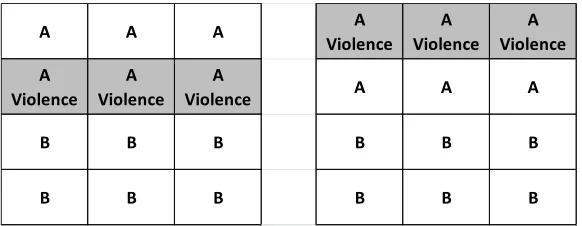
Conceptually, our approach aims to build a bridge between the cross-country con‡ict literature and the research using micro data. When cross-country studies link ethnic / religious diversity to con‡ict, their focus lies on the role of the overall size of di¤erent ethnic groups (i.e. ethnic polarization or fractionalization measures). This corresponds to making the implicit assumption that –for given …xed group population proportions– the average distance between members of the groups does not matter. Figure 1 illustrates the shortcomings of this assumption. Both the country of the left panel and the country of the right panel have the same number of regions (12) and the same level of nationwide population shares (with ethnic groups A and B being present in 6 regions each in both countries). However, in the left panel the average distance of a given region populated by A to the closest region populated by B is far greater than in the right panel where each of the six A regions is directly bordering some of the six B regions. When one assumes that the cost of committing attacks is increasing in the distance from the target, then the country in the right panel faces a higher expected number of attacks, despite the fact that it has the same population shares as the country to the left. Hence, our model can help to understand country heterogeneity in violence holding composition constant.
A A A A B A
A A A A A A
B B B B B B
B B B B A B
Figure 1: Two countries with the same ethnic composition but di¤erent spatial interaction
A A A A A A
A A A A A A
B B B
B B B B B B
B B B
Barrier
Barrier
Figure 2: Same level of segregation but di¤erent spatial interaction
interaction can be very di¤erent depending on the topology of the interaction (e.g. the location of barriers). Note that the logic is similar if for example instead of the existance of a barrier the population density varies across di¤erent regions. Con‡ict incentives would be smaller if low population density zones are located where the groups are close (i.e. in the second and/or third row of the left panel of Figure 1) than when they are located at places far away from other groups (i.e. in the …rst and/or fourth row of the left panel of Figure 1). Again, even for a similar degree of segregation, di¤erent locations of low and high population density areas can result in very di¤erent patterns of spatial interaction.
Figure 3 illustrates the idea behind our identi…cation strategy. The …gure shows a spatial distribution of ethnic groups A and B and two violence distributions. Violence, indicated by a grey shading, in the example on the left, is concentrated at the boundary between group A and B, while this is not the case in the right panel.
A A A ViolenceA ViolenceA ViolenceA
A Violence
A Violence
A
Violence A A A
B B B B B B
B B B B B B
Figure 3: Di¤erent violence patterns for the same group constellation
of violence with characteristic A. Yet, violence in the left panel could also be generated by attacks of B on A. Hence, ignoring the interaction between groups across space may result in misinterpretation and erroneous conclusions. Note also that running an existing standardspatial econometrics regression, such as a Spatial Durbin model (SDM), would not help if violence is indeed driven by theinteraction of A and B.
In a model with distance, the violence on the right is less likely to originate in group B. However, violence could also originate from group A in both cases. What we therefore use in the current paper to identify the e¤ect of distance is variation in the composition of regions and neighborhoods.
(Horowitz, 2000).4
In recent years there has been an increasing number of papers studying violence at a disag-gregate, local level (e.g. La Ferrara and Harari, 2012; Rohner, Thoenig, and Zilibotti, 2013b; Dube and Vargas, 2013; Berman et al., 2017; König et al., 2017), but most of these contributions do either not contain a formal model of con‡ict or do not take into account the local ethnic composition, usually due to data limitations.5 Also the micro-level literature on insurgency and counter-insurgency is relevant, see Kalyvas (2006), Lyall (2010), Bhavnani et al (2011), Kocher, Pepinsky and Kalyvas (2011), and Berman, Shapiro and Felter (2011).
Maybe closest to our contribution is the literature focusing on spatial patterns of violence. There is a small literature in political science studying –inspired by the epidemiological literature on the spread of diseases– di¤usion and clustering patterns of violence over space and time (Townsley, Johnson, and Ratcli¤e, 2008, Schutte and Weidmann, 2011). Further, Novta (2016) builds a simulation-based model of how con‡ict spreads. Contrary to our setting of insurgency and terrorism, her framework is designed to study traditional military warfare between two standing armies. The features of her model are found to be consistent with the spread of violence in the 109 municipalities of Bosnia. Novta models the armed groups in each municipality as separate, myopic players who can only attack in their home village while the focus of our framework lies precisely on the across-ward attacks.6 Bhavnani et al. (2014) link segregation to urban con‡ict, using a simulated agent-based model, calibrated for Jerusalem. Finally, the purely empirical contribution of Balcells, Daniels, and Escribà-Folch (2016) studies post-con‡ict sectarian clashes in Northern Ireland from 2005-2012. In a nutshell, a main di¤erence between our current paper
4
Sambanis (2000) concludes that partition does not signi…cantly prevent con‡ict.
5
There are also a few papers selecting an intermediate level of disaggregation and building a panel dataset
on the ethnic group level covering a large number of countries (e.g. Buhaug, Cederman, and Rod, 2008; Morelli
and Rohner, 2015; Esteban, Morelli and Rohner, 2015). However, their level of disaggregation is still much less
…ne-grained than in the current paper, and they do not focus on local ethnic cleavages and the interaction between
ethnic groups across regions.
and the existing work on spatial violence patterns is that –contrary to the existing literature–our empirical analysis estimates the structural parameters of a formal model of optimizing, farsighted players.
Finally, the predictive power of our framework is also useful when it comes to forecasting the impact of con‡ict on economic outcomes. Besley and Mueller (2012) show for Northern Ireland that compared to peaceful areas, housing in the most violent areas sold for between 2 and 17 percent less - depending on the level of violence, and Mueller (2016) shows that changes in the distribution of violence within a country have a very substantial impact on aggregate growth. Thus, predicting well the location of attacks does not only help in forecasting local economic outcomes, but also countrywide performance.
3
Model
In this section we provide a game-theoretic model of local violence, where two groups are in a contest about appropriating rents. In line with the con‡ict economics literature, the share of rents grabbed by a group depends on its relative …ghting e¤ort. In our setting, the two groups locally recruit …ghters for attacking a weighted average of opponents nearby. It turns out that this simple framework will allow us to predict the spatial distribution of violence in Northern Ireland to a stunning degree.
3.1 Set Up
In this one-period framework we model violence in a country with n regions indexed by i. In each region live two groups labelled, to …x ideas,g2 fc; pg. The population of groupgin region (ward)iisNig, wherei2 f1; :::; ng, and their distribution across regions can be expressed by
Ng = 0 B B B @
N1g
.. .
Nng
1 C C C A:
from the groupsg, denotedFig, forming
Fg = 0 B B B @
F1g
.. .
Fng
1 C C C A:
The central leaderships of each of the two paramilitary groups want to maximize the share of rentsR that they capture. These rents can be thought of as nationwide gains of holding power, which we assume to be private goods.
For the purpose of rent-maximization both group leaderships have to decide simultaneously on recruiting the optimal number of local …ghters in each region.
The share of rents captured by a group g is given by the following Tullock-form contest-success-function,
Ag Ag+A g;
where Ag are total attacks in‡icted by group g, A g are attacks in‡icted by group g. Note, that, in order to make the model solvable, we distinguish attacks from casualties which are a random outcome. In other words, we assume that the competition for rents is a¤ected by how many attacks the group makes and not how deadly they are.
Recruiting …ghters is costly. Typically, salary costs of …ghters should be thought of as convex, as the …rst few hirings will be cheap given that it will be feasible to target exclusively individuals with low wages in the regular economy (and hence low opportunity costs of …ghting) and/or with low moral costs of killing. When extending the pool of …ghters in a region, the group also needs to recruit individuals with better outside options and higher moral costs who will require higher monetary compensation.
Further, the larger the population of locals of a given group in a given region the cheaper the hiring costs, as the …ghters face lower risks of identi…cation and being arrested and can bene…t from more local support and safehouses.
1 2
(Fig)2
(Nig) ;
where 0:
This functional form has several advantages. First of all, using a square term of the e¤ort variable (and normalizing by1=2) is the simplest way of capturing convexity, and has been used in a large number of contributions in di¤erent …elds of economics. Second, the term (Nig) is very ‡exible: If = 1, then the costs of recruiting for groupg drop with higher population from groupg; if = 0, local support doesn’t matter in the sense that the costs of recruiters scales only with the total number of …ghters in the region. We …nd that 1yields the best …t to the data which indicates that local support for the …ghting e¤ort is important.
The number of attacks is a function of the available targets and their proximity. We model interaction across space ‡exibly by de…ning a group-speci…c symmetric spatial weights matrix
Wg = Wg1 Wgn =
0 B B B @
wg11 w1gn
..
. . .. ...
wng1 wgnn
1 C C C A
with wgij = wjig for all i; j. The spatial weight wijg parametrizes how costly it is for group g
to project violence from region i to region j. The number of attacks perpetrated by group g
emanating from location iare given by
Agi =Fig
n
X
j=1
wijNj g =F g
i (W
g
i)0N g; (1)
where g denotes the opposite group. This means that attacks launched from i by g are the interaction of the number of perpetrators (…ghters) in i and the spatially weighted number of potential victims (population) in all regions. Thus, overall attacks by groupg are
Ag =
n
X
i=1
Agi = (Fg)0(Wg)N g:
Putting these elements together, the payo¤ function of a groupg’s leadership becomes
g= Ag
Ag+A gR
1 2
n
X
i=1
(Fig)2
3.2 Characterization of the Equilibrium
The equilibrium is determined by the number of …ghters that each group recruits in each region. Each group has to optimally select recruiting numbers for every region,Fig, given the number of …ghters that the other group recruits. Hence, we will obtain a system of2 n…rst-order conditions (FOC) and2 nunknowns. Given that in each FOC the bene…ts of a marginal recruit (i.e. the …rst term) are strictly concave, while the marginal costs (i.e. the second term) are strictly convex, the second-order conditions (SOC) hold and there is a unique interior equilibrium.
The marginal …ghting strength increase of an additional …ghter of group g in region i corre-sponds to
@Ag
@Fig = (W
g
i)0N g;
which implies that the incentive to recruit …ghters locally will be a weighted function of the possible targets for those …ghters. For each regioni we therefore get a FOC, which for group g
is given by
@ g @Fig =
(Wgi)0N gA~ g
~
Ag+ ~A g 2
R F~
g i
(Nig) = 0;
whereA~g,A~ g andF~ig are equilibrium values. The optimal choice of local …ghting e¤ort satis…es
~
Fig = A~
g
~
Ag+ ~A g 2
R (Wgi)0N g(Nig) : (2)
Equation (2) says that local …ghting e¤ort is a function of a part which is constant across all regions, A~ g
(A~g+ ~A g)2R, and a part which varies from region to region(W
g
i)0N g(N g
i) . Note, that
(Wig)0N g(Nig) is the weighted sum of all population in group g interacted with(Nig) . The easier it is to recruit, i.e. the higher(Nig) , the more …ghters will be recruited locally. Further, the more targets are in reach, i.e. the higher(Wgi)0N g, the more …ghters will be recruited.
In the empirical analysis we will be able to make use of the fact that the relative …ghting e¤ort between regions is only a function of demographic exogenous variables and the e¤ectiveness of …ghting captured by the spatial weightswgij. While the absolute magnitude of thewijg parameters is di¢ cult to interpret, one should expect all wijg 0; and wgi0j < wijg if dist(i0; j) > dist(i; j), and wijg0 < w
g
ij if dist(i; j0) > dist(i; j). In other words, we expect e¤ectiveness to decrease in
Given the equilibrium number of …ghters originating from each region it is easy to calculate the number of attacks targeted at each region. Casualties of groupg in regioniare given by
casgi =Nig Wi g 0F~ g+"i; (3)
whereF~ g is the vector version of equation (2) given by
~
F g= A~
g
~
Ag+ ~A g 2
R diagh W g 0Ngi(N g) ; (4)
where (N g) is an element-by-element exponent and diagh(W g)0Ng i
is a matrix with the values of (W g)0Ng on the diagonal and zero otherwise.7 The error term "i, with E("i) = 0,
in equation (3) re‡ects the fact that there is some randomness in the transmission from attacks to casualties. Not all successfully carried out attacks do result in the same number of fatalities, which is the variable observed by the econometrician.
Equation (3) captures the essence of our theory. Violence at location i is the result of an interaction between targets in locationi,Nig, and the number of attackers based in all locations,
~
F g. How dangerous these interactions are for the population at i depends on the vector of weightsWi g. Note, however, that the full weighting matrix for all locations,W g, also plays a role (throughF~ g) because it determines how many …ghters are recruited by the other group.
Thus, a general fall in transport costs (increase in wijg) has two e¤ects. First, …ghters in the neighborhood ofiare more e¤ective and therefore attack more in regioni. This is the e¤ect coming from Wi g in equation (3). Second, more …ghters are recruited in all other locations because they can attack more e¤ectively in their respective neighborhoods. This e¤ect is captured by the matrixW g in equation (4).
7
We haveF~ g= A~g (A~g+ ~A g)2R
0 B B B @
N1gw11g+N2gw21g:::+Nngw g
n1 0
..
. . .. ...
0 N1gw1ng+N2gw2ng:::+Ng nwnng
1 C C C A 0 B B B @
4
Empirical Implementation: The Data
The structural parameters of the model are estimated using data from the con‡ict in Northern Ireland. This is one of the most important and costliest con‡icts in a developed country over the last decades. Studying the Northern Irish "Troubles" allows us to draw on very …ne grained group location and …ghting event location data. Below we shall start by describing the context of this con‡ict, before providing a detailed description of the data used.
4.1 Context of Con‡ict in Northern Ireland
The Northern part of Ireland, Ulster, has been religiously divided since its conquest by England and the Reformation, taking both place in the 16th century.8 Since then the Catholic
popu-lation from Gaelic Irish origin and the Protestant popupopu-lation of English and Scottish settlers have lived "separate lives" characterized by very stable patterns of land holdings and relatively few religiously mixed marriages (Mulholland, 2002). When the Republic of Ireland achieved independence from Britain in 1922, the six Northern counties of Ireland remained part of the UK.
In the early 1920s "Troubles" broke out with the Irish Republican Army (IRA) challenging British authority over Ulster and engaging in violent combats against the British troops and Protestant paramilitary organizations such as the Ulster Volunteer Force (UVF). The following decades were characterized by "home rule" and the new Parliament of Northern Ireland at Stor-mont near Belfast. The political divide persisted between the Catholic Nationalists (also called Republicans) who wanted to join the Republic of Ireland and the Protestant Unionists (also called Loyalists) who wanted to remain united with the UK.
While in the 1950s and early 1960s there were relatively low levels of political violence, in 1968 the situation became again more confrontational when the Civil Rights Movements asked for more rights for Catholic citizens. Some of the initially peaceful demonstrations and marches
8
were met with repression and resulted in fatalities. From August 1969 onwards sectarian violence exploded. In September 1969 radical militants took control of the previously dormant IRA and created its radical wing, the Provisional IRA. The "Provos" achieved an ever tighter grip over traditional Catholic working class strongholds like the Falls Road in Belfast or the Bogside in Derry.
Further, alarmed by the rise of the IRA and the seeming willingness of the UK government to make political concessions, loyalist paramilitary organizations stepped up in the 1970s, intimidat-ing Catholic families from mixed and Protestant areas and startintimidat-ing a violent campaign against civilian Catholics.
After 1976 the UK built up a stronger Royal Ulster Constabulary (RUC) that together with the British Army and the SAS troops stepped up e¤orts to militarily weaken the IRA. This e¤ort led the loyalist paramilitaries to lower their violence and the IRA to retrieve from large-scale open confrontations and to adopt a cellular structure common in terrorist organizations.
Even carefully planned attacks by the paramilitary groups had to rely on operational centres based on religion. Dillon (1999), for example, describes an IRA operation in October 1972 as follows:
"The intelligence o¢ cer of the 1st Battalion said Twinbrook was the best for an assault on
the laundry van [...]. He reckoned that if the van was attacked in Twinbrook an IRA unit could
make an escape with ease and be in the safety of the Andersontown district within a matter of
…ve to ten minutes."(Dillon 1999, page 42).
In Andersontown the 1971 census counted 5588 Catholics and 51 Protestants. The quote shows that the IRA was operating from and around this Catholic ward. This made attacks on Protestants and state forces close to Andersontown more likely.
4.2 Data from Northern Ireland
data in the description of killings to derive geo-references data. We then use these references to match killings to wards and grid-cells. The violence data is unique as it reports the religion of each victim (unless for members of the state forces) and the group that attacked him or her.
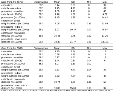
We have data on 582 wards (our unit of analysis), which are regrouped into 101 larger District Electoral Areas (DEA) which again map into 26 local government districts.9 Table 1 shows the summary statistics of the most relevant variables. The number of Catholics and Protestants are in thousands. Table 1 also summarizes our data on con‡ict-related casualties. The special feature of this data is that it reports the group a¢ liation of victims of violence.
We …rst notice that while the average number of casualties per ward is relatively small, the variance is very large. While in many wards no fatalities occur, the most violent ward records 97 casualties. We further see that casualties are relatively evenly split between catholic and protestant victims and that there is a large heterogeneity in the group composition of wards and their neighborhood.
In our main analysis we focus on the settlement patterns and violence data from the 1970s, when most of the violence takes place. Table 1 shows that there are 3.14 casualties on average per ward in the 1970s and 1.25 casualties in the 1980s. In a sensitivity test, we also show robustness of the …ndings when including the 1980s. We focus on the …rst decade (1970s) to ensure that reverse causality between settlement patterns and violence are less of a concern. Since the census data is from the start of the respective decade we should be able to capture the e¤ect of settlement patterns before violence broke out. It is much harder to argue this for the 1980s or 1990s.
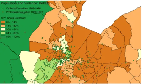
Figure 4 below illustrates the type of data we use, focusing on a part of Belfast for a particu-larly violent period of the con‡ict (1969-1976). Our data contain information on the demographic composition of all administrative wards (with the white area in the upper-right corner depicting the sea), as well as information on the location and religious a¢ liation of all recorded fatalities.
9The wards are from the District Electoral Areas (Northern Ireland) Order 1993. These boundaries
have been revised in 2014. A list of 1993 wards and their corresponding DEAs can be found under
Data from the 1970s Observations Mean SD Min Max
casualties 582 3.14 8.63 0 97
catholic casualties 582 1.45 4.71 0 62
protestant casualties 582 1.69 4.46 0 46
catholics (in 1000s) 582 1.18 1.08 0 9.72
protestants (in 1000s) 582 1.45 1.88 0 14.42
catholics in direct
neighbourhood (in 1000s) 582 7.08 4.91 0.36 32.84 protestants in direct
neighbourhood (in 1000s) 582 8.07 10.37 0.00 76.97 catholics in two wards
distance (in 1000s) 582 16.45 9.46 0.92 51.25
protestants in two wards
distance (in 1000s) 582 18.32 21.77 0.21 138.51
Data from the 1980s Observations Mean SD Min Max
casualties 582 1.25 2.54 0 19
catholic casualties 582 0.48 1.36 0 11
protestant casualties 582 0.77 1.61 0 13
catholics (in 1000s) 582 1.44 0.84 0.04 5
protestants (in 1000s) 582 1.07 1.33 0.00 7
catholics in direct
neighbourhood (in 1000s) 582 8.61 4.40 1.04 23
protestants in direct
neighbourhood (in 1000s) 582 5.82 7.24 0.00 45
catholics in two wards
distance (in 1000s) 582 19.74 9.78 1.86 58
protestants in two wards
distance (in 1000s) 582 13.09 15.61 0.00 97
Notes: From CAIN (2015), Sutton (1994) and NISRA (2015). We code casualties of the state forces as protestant casualties if a ward has casualties whose religion is not revealed.
Figure 4: Map of inner Belfast wards with information on demographics and fatalities
In line with our theory we see that many fatalities take place in either religiously mixed wards or in religiously homogeneous wards located close to strongholds of the other religious commu-nity. In contrast, religiously homogenous wards located far away from the other religious group experience only small levels of violence.
5
Estimations
5.1 Estimation of the decay of distance parameters
One unique feature of our setting and data is that it allows us to estimate the decay of distance parameters captured by the spatial weights matrixWg.
the …rst degree. In a second step, we will also consider violence between higher degree neighbors. For the empirical estimation, we shall assume that the spatial weight for within-ward interac-tions is the same in all wards, i.e. wgii=wgjj. Similarly, the spatial weight for direct neighboring wards is assumed to be the same for all neighbor pairs, i.e. if i; j; l are a triad of neighboring wards, thenwijg =wilg =wjlg. For simplicity, we label these coe¢ cients of interest of the spatial weights matrixWg askg0,g=fc; pg;for within-ward violence (i.e. wherewgij hasi=j), and as
k1g for direct neighboring wards (i.e. with wijg whereiand j are direct neighboring wards). With these assumptions we can simplify equation (3). Call n1(j) the neighboring wards of
j. We can then write casualties su¤ered by groups p orcin ward j as a function of targets,Njg, interacted with the number of attackersF~j g and F~i2gn1(j), i.e. we can write
caspj = Njp Wjc 0F~c+"j (5)
= Njp
0
@k0cF~jc+k1c X
i2n1(j)
~ Fic
1 A+"j;
cascj = Njc 0
@kp0F~jp+kp1 X
i2n1(j)
~ Fip
1
A+"j; (6)
where the equilibrium number of attackers in each location is given by
~
Fjc = A~
p
~
Ac+ ~Ap 2
[(kc0Njp+k1c X
i2n1(j)
Nnp1(i))(Njc) ]; (7)
~ Fjp =
~ Ac
~
Ac+ ~Ap 2
[(kp0Njc+k1p X
i2n1(j)
Nnc1(i))(Njp) ]: (8)
Note, that equations (7) and (8) indicate that the recruitment of attackers is driven by the respective neighborhood. This implies that, in order to estimate equations (5) and (6), we need data for the composition of the direct neighborhood and data for the composition of the neighbor’s direct neighborhood. Variation in the neighborhood composition is essential for our identi…cation strategy.
(1) (2) (3) (4)
VARIABLES protestant casualties protestant casualties catholic casualties catholic casualties
k0 10.88*** 9.98*** 10.48*** 9.68**
(0.93) (1.43) (2.79) (4.51)
k1 1.77*** 1.20*** 2.94*** 1.63
(0.11) (0.40) (0.38) (2.44)
k2 0.41 0.91
(0.35) (0.94)
p value: k0=k1 0.00 0.00 0.02 0.23
p value: k0=k2 . 0.00 . 0.02
p value: k1=k2 . 0.29 . 0.83
Observations 582 582 582 582
R-squared 0.61 0.61 0.76 0.77
Notes: Robust standard errors in parentheses. Standard errors are clustered at the electoral district level (101 clusters). *** p<0.01, ** p<0.05, * p<0.1. "Protestant casualties" are casualties of state forces and protestants. "Catholic casualties" are casualties of catholics. The model's parameter "mu" (determining how the recruitment of fighters relies on local population) is normalized to 1. "k0-k2" are decay parameters. k0 captures the transport cost of conducting attacks within the same ward. k1 captures the transport cost of conducting attacks in the direct (bordering) neighbourhood of the ward. k2 captures the transport cost of crossing one ward to carry out an attack. In columns (1) and (2) we report the k parameters of catholic paramilitaries and in columns (3) and (4) we report the k parameters of protestant armed groups.
Table 2: Main estimation of the spatial weight parameters, separately for protestant and catholic casualties
by protestant …ghters. This bringsA~c+ ~Ap as close as possible to the total number of casualties while still using information on the violence perpetuated by the two sides in the con‡ict.
Table 2 displays the results of our estimates of the spatial weight parameters in our model. The parameter k0g captures the e¤ectiveness of attacks within the same ward, k1g captures the e¤ectiveness of attacks in the direct (bordering) neighborhood of the ward, and k2g captures the e¤ectiveness of attacks of second-degree neighbors. We estimate the expressions for caspj, and
casc
j, from equations (5) and (6), respectively, running a non-linear regression (see Davidson and
MacKinnon, 1993) and let the estimator pick the values of k0g, k1g, and kg2 that maximize the …t.10 Focussing in column (1) on violence against Protestants and onkc0andkc1only, we …nd that
1 0We use non-linear-least squares to …t the equation. We have also estimated parameters with maximum
like-lihood under the assumption of a negative binomial (overdispersion is a clear problem in the data). Results are
qualitatively similar with precisely estimatedk0,k1 andk0> k1 but point estimates are lower and the model …t is
all k-coe¢ cients are precisely estimated (both signi…cant at the 1 percent level) and that kc
0 is
substantially larger thank1c, showing a clear decay. In line with our hypotheses, there is indeed a cost of projecting violence over distance, and the attacks decay across ward borders. According to the estimates of column (1), the violence potential originating from a given ward is about six times smaller when the ward border needs to be crossed than within-ward.
In column (2), also second degree neighboring wards are included in the analysis (k2c). Again, thek-coe¢ cient gradually decreases when crossing an additional ward border, displaying a clear-cut ranking ofkc
2 < kc1 < kc0. Columns (3)-(4) display similar estimations for catholic casualties.
The coe¢ cients ofk0p andk1p are somewhat comparable to the ones found for protestant fatalities in columns (1)-(2), and the ratio of kg1=k0g is of a similar magnitude (i.e. roughly four) as in columns (1)-(2) (i.e. roughly six). In column (4) we again include second degree neighboring wards. While the qualitative picture of column (4) is very similar to column (2), the coe¢ cients are less precisely estimated.
It is important to stress that the similarity of results in columns (1) and (3) are not a given. Many wards had large catholic or protestant majorities so that population composition varied dramatically between Protestants and Catholics in 1971. This means that the variation used to identify the parameterskc0 and k1c is quite di¤erent to the variation used to identifykp0 andk1p.
As mentioned above, in Table 2 we have normalized the model’s parameter (that determines how the recruitment of …ghters relies on local population) to 1. Given that it seems di¢ cult to …nd a reliable proxy for , this is a reasonable way of proceeding. We include two additional robustness tables, relaxing this normalization. First, we perform a maximum likelihood grid search, yielding the value of that maximizes the overall …t of the model. The results are displayed in Table 9 in Appendix B, which replicates Table 2, but using the found in the grid search. First of all, note that in all four columns the found is always in the neighborhood of 1, ranging from 0.78 to 1.18. Second, the estimated coe¢ cients of k0g, k1g, and k2g are similar in terms of size to the ones found in the baseline Table 2.
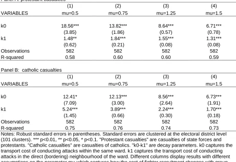
0:5; = 0:75; = 1:25 and = 1:5. Panel A reports the results for protestant casualties and Panel B reports the results for Catholic casualties. The relative size of the coe¢ cients changes but k1g < k0g is always maintained. The estimated parameters fall for larger values of . This can be explained by the fact that higher values of imply more …ghters per population. If the number of …ghters increases, e¤ectiveness of these …ghters needs to decrease in order to maintain the level of violence. Also, estimates fork0g fall relative tok1g for larger values of . This change is driven by large mixed wards which generate a lot more within-ward violence for large due to the non-linearity in the recruitment technology. Note that we …nd that catholic casualties are best described (highest R2) by a slightly lower (close to 0:75 as opposed to close to 1:25 for protestant casualties). This could be explained by the fact that protestant …ghters include state forces which we expect to move more freely and therefore are less bound by local support by Protestants.
Our framework also allows us to estimate the total combined death toll of Protestants and Catholics,casj caspj+cascj, relying again on the structural equations (5) and (6). This is what
we do in Table 4. In particular, we allow for di¤erent kmc 6= kmp, but assume that the relative
decay of distance is similar for both population groups, i.e. kcm=kmc =kmp =kmp, for m = 1;2:::M.
This is reasonable in the light of Table 2 that indeed found for both population groups similar spatial weight ratios of k0=k1, and k1=k2. It implies that we can replace the ratio kmc=k
p
m by a
constant for allm. CallMc (kcm=k p
m)2. We can then write casualties in wardj as
caspj +cascj = Mc Njp
0
@kp0F~j0c+k1p X
i2n1(j)
~ Fi0c
1
A (9)
+Njc
0
@kp0F~jp+kp1 X
i2n1(j)
~ Fip
1 A+ j;
where j is the error term of the combined regression, Fip is given by equation (8), and F~i0c
corresponds toF~ic of equation (7) besides the fact that kmc is replaced bykpm.
This combined estimation of casj also allows us to compute the relative "aggressiveness of
catholic paramilitaries compared to state forces and loyalist paramilitaries", captured by the pa-rameterMc, which intuitively tells us how many attacks are carried out by Catholics compared to
paramil-Panel A: protestant casualties
(1) (2) (3) (4)
VARIABLES mu=0.5 mu=0.75 mu=1.25 mu=1.5
k0 18.56*** 13.82*** 8.64*** 6.71***
(3.85) (1.86) (0.57) (0.78)
k1 1.48** 1.84*** 1.55*** 1.31***
(0.62) (0.21) (0.08) (0.08)
Observations 582 582 582 582
R-squared 0.58 0.60 0.60 0.59
Panel B: catholic casualties
(1) (2) (3) (4)
VARIABLES mu=0.5 mu=0.75 mu=1.25 mu=1.5
k0 12.41* 12.13*** 8.56*** 6.73***
(7.09) (3.00) (2.64) (1.91)
k1 5.24*** 3.89*** 2.24*** 1.70***
(1.45) (0.66) (0.30) (0.18)
Observations 582 582 582 582
R-squared 0.75 0.76 0.74 0.73
Notes: Robust standard errors in parentheses. Standard errors are clustered at the electoral district level (101 clusters). *** p<0.01, ** p<0.05, * p<0.1. "Protestant casualties" are casualties of state forces and protestants. "Catholic casualties" are casualties of catholics. "k0-k1" are decay parameters. k0 captures the transport cost of conducting attacks within the same ward. k1 captures the transport cost of conducting attacks in the direct (bordering) neighbourhood of the ward. Different columns display results with different assumptions on the parameter mu which captures how the cost of fighter recruitment changes with group size.
itaries carry out less attacks than protestant …ghters for a given availability of targets, while
Mc >1 implies that catholic …ghters are relatively more "aggressive". The interpretation of Mc
of course requires caution, as anyMc6= 1 could be due to various factors such as e.g. di¤erences
in motivation, organization or logistical capacity of paramilitary groups, di¤erences in population support, advantages and constraints related to being linked to the political establishment etc. Our data do not allow us to disentangle the root causes driving the value ofMc.
Table 4 performs this joint estimation of total casualties, and shows that indeed there is a gradual decay of attack potential when crossing ward borders, with all k-coe¢ cients being statistically signi…cant andkp2 < kp1 < k0p. It is particularly re-assuring that the point estimates are very close to the estimates ofk2p; k1pandk0pin Table 2. Further, theMccoe¢ cient is estimated
to be around 0.6, revealing that for an identical availability and proximity of targets, assuming everything else constant, catholic paramilitaries carry out roughly 20 percent less attacks than protestant forces.11
A crucial aspect to keep in mind is that, while k0p > k1p, the latter parameter applies to a lot more interactions. The neighborhood contains a population that is more than …ve times larger than the population of the average ward. This implies that more than half of all attacks, according to the speci…cation of Table 4, take place across ward boundaries.12
5.2 Comparison to Alternative Models
A clear advantage of modeling the local interaction of the local population is a gain in the explanatory power of the model. In order to show this we consider two benchmarks. The …rst benchmark is an alternative framework where only ward population characteristics matter and where, accordingly, the violence potential is assumed to fully decay when a ward-border is crossed. Put di¤erently, this corresponds to a setting often encountered in within-country studies in which the location of attacks and targets is not separated.
1 1
We calculate this fromkcm=kmp =
p
0:63 = 0:79:
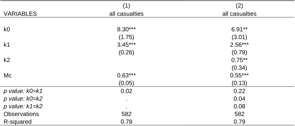
(1) (2)
VARIABLES all casualties all casualties
k0 8.30*** 6.91**
(1.75) (3.01)
k1 3.45*** 2.56***
(0.26) (0.79)
k2 0.75**
(0.34)
Mc 0.63*** 0.55***
(0.05) (0.13)
p value: k0=k1 0.02 0.22
p value: k0=k2 . 0.04
p value: k1=k2 . 0.08
Observations 582 582
R-squared 0.78 0.79
Notes: Robust standard errors in parentheses. Standard errors are clustered at the electoral district level (101 clusters). *** p<0.01, ** p<0.05, * p<0.1. The model's parameter "mu" (determining how the recruitment of fighters relies on local population) is normalized to 1. "k0-k2" are decay parameters. k0 captures the transport cost of conducting attacks within the same ward for state forces and loyalists (kp0 in the text). k1 captures the transport cost of conducting attacks in the direct (bordering) neighbourhood of the ward for state forces and loyalists. k2 captures the transport cost of crossing one ward to carry out an attack for state forces and loyalists. Mc captures the relative aggressiveness of republican paramilitaries compared to state forces and loyalists, (kc/kp)^2.
We model this alternative by regressing ward-level casualties on the numbers of Protestants and Catholics in a given ward and their interaction. In Appendix B, Table 10 depicts the regression results for this alternative speci…cation in column (1).13
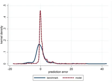
Figure 5 below displays a comparison of our setting (called "model") with the benchmark alternative model of full distance decay of the Appendix Table 10, column (1) (called "bench-mark"). The curves represent the distribution of the residuals, i.e. casj cascj. Large numbers
mean that the extent of violence is underestimated. In the benchmark model we predict violence with the population composition and interactions within the ward, whereascascj in our model is
given by the …tted values from equation (9). The curve capturing our model is drawn in a dashed red line, while the benchmark curve is drawn in a blue solid line. The curve of our setting is centered around zero and reaches a very high kernel density close to zero. This reveals that the …t is very good, with most wards having very similar levels of actual and …tted casualties. In contrast, the alternative model has a substantially lower …t, revealed by a larger spread away from zero (running an F-test con…rms at the 1% level of signi…cance that the alternative benchmark has a larger standard deviation of the error terms). The alternative model slightly overestimates violence in a large number of wards and grossly underestimates it in a few other wards. This is not only a result of not taking cross-border attacks into account but also of ignoring the changes in motivation to …ght in areas with a lot of potential targets.14
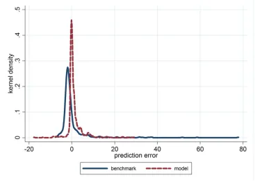
The second natural benchmark to consider is a model assuming no decay of violence potential over space. This is the implicit assumption of many country-level studies assuming that only the overall population composition but not their location matters (see Figure 1). According to this "no spatial decay" benchmark the population composition in a given ward and in its neighborhood
1 3In column (2) of the Appendix Table 10 we display another alternative speci…cation which is also common in
the literature. This speci…cation ignores population size and predicts casualties with the share of catholics and its
square. This speci…cation has almost no predictive power.
1 4
To see this, imagine that k1 is set to 0. This has two e¤ects: First, even if the recruitment of …ghters
was unchanged, their e¤ectiveness would decrease. Second, the e¤ect is anticipated and recruitment of …ghters
Figure 5: Our model compared to full decay
should only a¤ect casualties through the nationwide presence of potential victims, i.e. this boils down to settingk0 =k1 =k2:::=kn. Attacks are then given by
c
casgj = N
g j
P
jN
g j
~ A g:
This simply means that total casualties of groupgwill be distributed according to where groupg
lives. From this we can calculatecascj =casccj+casc p
j and casj cascj. In Figure 6 we compare the
…t of our setting (called "model", depicted by the red dashed curve) with this no decay benchmark (called "benchmark", displayed by the blue solid line). This reveals a substantially less good …t of the no decay benchmark, with violence in many wards being drastically underestimated (running an F-test con…rms at the 1% level of signi…cance that the alternative benchmark has a larger standard deviation of the error terms).
5.3 Robustness checks
Figure 6: Our model compared to no decay
Table 5 shows that the statistical inference is robust to various levels of clustering standard errors. One natural alternative option for clustering would be at the parliamentary constituency or district level, although unfortunately the number of parliamentary constituencies and districts are only 18 and 26, respectively, which is below the typical lower bound of clusters required (50). Incidentally, if we ignore this issue and still cluster at these levels, as we do in columns (1) and (2) of Table 5, the signi…cance is maintained at the 1 percent level for all coe¢ cients. In column (3) we show that the results are also robust when clustering is absent altogether.15
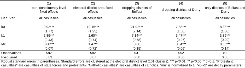
Table 6 shows that the results continue to hold when …xed e¤ects are included or particular parts of Northern Ireland are excluded. In columns (1) and (2), we include …xed e¤ects at the parliamentary constituency, resp. electoral district level. The magnitude and statistical signi…cance of the estimates remains very similar to our baseline results. In column (3) the Belfast area is dropped from the sample. This was by far the most violent part of Northern
1 5
We have also checked out the sensitivity to clustering by the coordinates of the wards and on a combination
(1) (2) (3) errors clustered at
parl. constituency level
errors clustered at district council level
no clustering
VARIABLES all casualties all casualties all casualties
k0 8.30*** 8.30*** 8.30***
(1.80) (0.55) (3.01)
k1 3.45*** 3.45*** 3.45***
(0.28) (0.06) (0.54)
Mc 0.63*** 0.63*** 0.63***
(0.10) (0.03) (0.14)
Observations 582 582 582
R-squared 0.78 0.78 0.78
Robust standard errors in parentheses. *** p<0.01, ** p<0.05, * p<0.1. "Protestant casualties" are casualties of state forces and protestants. "Catholic casualties" are casualties of catholics. "mu" is normalized to 1. "k0-k2" are decay parameters. k0 captures the transport cost of conducting attacks within the same ward. k1
captures the transport cost of conducting attacks in the direct neighbourhood of the ward. k2 captures the transport cost crossing one ward to conduct an attack. Mc captures the relative aggressiveness of republican paramilitaries compared to state forces and loyalists (as detailed in the text). There are 18 parliamentary
constituencies and 26 district councils.
(1) (2) (3) (4) (5) parl. constituency level
fixed effects
electoral district area fixed effects
dropping districts of
Belfast dropping districts of Derry
only districts of Belfast and Derry Dep. Var. all casualties all casualties all casualties all casualties all casualties
k0 9.92*** 10.15*** 21.92*** 7.88*** 8.38*** (1.77) (1.95) (7.14) (1.66) (1.80) k1 2.89*** 1.60** 7.14*** 3.47*** 3.39***
(0.43) (0.74) (0.78) (0.27) (0.29) Mc 0.68*** 1.47** 0.08 0.64*** 0.65***
(0.07) (0.72) (0.15) (0.06) (0.14) Observations 582 582 531 552 81 R-squared 0.83 0.87 0.38 0.80 0.86 Robust standard errors in parentheses. Standard errors are clustered at the electoral district level (101 clusters). *** p<0.01, ** p<0.05, * p<0.1. "Protestant casualties" are casualties of state forces and protestants. "Catholic casualties" are casualties of catholics. "mu" is normalized to 1. "k0-k2" are decay parameters. k0 captures the transport cost of conducting attacks within the same ward. k1 captures the transport cost of conducting attacks in the direct neighbourhood of the ward. k2 captures the transport cost crossing one ward to conduct an attack. Mc captures the relative aggressiveness of republican paramilitaries compared to state forces and loyalists (as detailed in the text). There are 18 parliamentary constituencies and 101 electoral district areas.
Table 6: Fixed e¤ects and alternative location samples
Ireland with more than 850 casualties. The decay of violence across distance is still clear-cut, withk1< k0 still holding, and bothk0 andk1 being highly statistically signi…cant. In column (4)
we drop Derry, the second most violent area from the sample. In column (5) we include instead in the sample only the wards of Belfast and Derry. In all cases our results continue to hold. This shows that our …ndings are not driven by particular regions within Northern Ireland.
Further, Table 7 considers alternative time frames. Using religious group settlement patterns and violence data from the 1970s was the natural choice for the baseline regressions, as this re‡ects pre-con‡ict location decisions, which are arguably more exogenous than the people’s location choices in the 1980s. Still, in Table 7 we show robustness of our main results to the inclusion of data from the 1980s. In particular, in columns (1) and (2) we use data from the 1970s and 1980s to show that parameters do not change signi…cantly from one decade to the next. In particular, in column (1) we …rst estimate the same set of parameters as in the baseline regressions, but for a larger sample containing also data from the 1980s, leading to a similar overall pattern as in the baseline regressions. Then we estimate in column (2) the di¤erence between parameters in the 1970s to 1980s.16 To do this we run a regression in which we separate the 1970s and 1980s through two sets of spatial weight dummies. We use “k0 in the 80s”= “k0in
(1) (2) (3)
70s and 80s pooled data
70s and 80s pooled data
placebo test (80s census, 70s
violence)
VARIABLES all casualties all casualties all casualties
k0 9.56*** 9.61*** -14.85
(2.24) (2.03) (15.14)
k1 4.01*** 3.99*** 11.17***
(0.39) (0.31) (1.20)
k0 change - 80s -2.49
(8.78)
k1 change - 80s 0.50
(1.10)
Mc 0.68*** 0.69*** 0.50***
(0.07) (0.06) (0.17)
Mc change - 80s -0.19
(0.23)
Observations 1,164 1,164 582
R-squared 0.75 0.75 0.67
Notes: Robust standard errors in parentheses. Standard errors are clustered at the electoral district level (101 clusters). *** p<0.01, ** p<0.05, * p<0.1. The model's parameter "mu"
(determining how the recruitment of fighters relies on local population) is normalized to 1. "k0-k2" are decay parameters. k0 captures the transport cost of conducting attacks within the same ward. k1 captures the transport cost of conducting attacks in the direct (bordering) neighbourhood of the ward. Mc captures the relative aggressiveness of republican paramilitaries compared to state forces and loyalists (as detailed in the text).
the 70s”+ “k0 change 80s”to replace for “k0 in the 80s”in the regression equation and estimate
twok0 parameters: “k0 in the 70s” and “k0 change 80s”. We do the same for thek1 parameters
and Mc. We do this in order to be able to conveniently test whether parameters changed from the 1970s to the 1980s, …nding that coe¢ cients are stable over time.
The fact that estimates over di¤erent decades are similar could be due to either the structure of our model applying to various periods, or, alternatively, due to the fact that population movements across Northern Ireland are limited. To discriminate between these two explanations, we perform a placebo test in column (3). Concretely, we try to explain the violence in the 1970s with settlement patterns in the 1980s. If the composition of the population is highly persistent we should …nd the same result as in the previous two columns, while if population movements are substantial the placebo test should generate results that are not in line with the …rst two columns. This is exactly what we observe in column (3), suggesting that the stability of the estimates in columns (1) and (2) is not driven by the absence of population movements. This is consistent with the view that indeed the structure of our model applies to various sub-periods of the "Troubles" in Northern Ireland.
6
Uses of the Model for Prediction
Our model builds on the assumption that the starting position of an attack is separated from the location of the attack. Given the parameter estimates of the model from the previous section, we can "invert" the model to calculate where attacks came from and which path they took. It is di¢ cult to overemphasize the importance of this for the use of disaggregated data. The more disaggregated the data is, the more often will the location of a target and the origin of violence di¤er. Especially for the analysis of and response to sectarian violence taking this into account can be crucial.
changes in the spatial composition of population reduced violence dramatically, despite the fact that total population did not change as much.
6.1 Predicting the Origin of Attacks
Our model enables us to compute the expected size of bilateral attacks from any ward against any other ward. Generally, we are able to calculate the number of attacks originating in a given wardj from equation (1) as
Aj = ~Fjc Wcj 0Np+ ~F p
j W
p j
0
Nc: (10)
In the simpli…ed model in Table 4, column (1) we have estimated three parameters. From these we can calculate the number of attacks on other, contiguous wards that originated in ward
j as
^
Aj = ^Fjc M^c k^p1
X
i2n1(j)
Nip+ ^Fjp k^p1 X
i2n1(j)
Nic; (11)
and the number of attacks that came into the ward from a di¤erent ward as
c
caspj +casccj =Njp M^c k^p1
X
i2n1(j)
^
Fi0c+Njc k^p1 X
i2n1(j)
^
Fip; (12)
where, in both cases, we use the (…tted) number of attackers in each location is given by
^
Fjc = A~
p
~
Ac+ ~Ap 2
[(^kc0Njp+ ^k1c X
i2n1(j)
Nnp1(i))(Njc) ];
^
Fjp = A~
c
~
Ac+ ~Ap 2
[(^kp0Njc+ ^k1p X
i2n1(j)
Nnc1(i))(Njp) ]:
The subtle di¤erences between equation (11) and equation (12) illustrate the intuition of the empirical model. While casualties in equation (11) (i.e. deaths caused) are calculated by multiplying the number of …ghters in wardjwith the sum of potential targets in the neighborhood, casualties in equation (12) (i.e. deaths su¤ered) are calculated by multiplying the number of targets in wardj with the sum of …ghters in the neighborhood.
0
20
40
60
80
1
00
at
tack
s fro
m w
ard
0 20 40 60 80
attacks in ward
Figure 7: Origin and destination of attacks in the 1970s.
close to the 45 degree line while "net contributors" (i.e. wards that create more violence than they su¤er) are located above the 45 degree line.17
An interesting feature of Figure 7 is that wards with low levels of violence tend to receive more attacks than they commit. However, this reverses for violent wards. This pattern is a feature of a model in which recruitment of …ghters,Fjg, is endogenous. Wards with a large population will generate higher F~jg and attack surrounding wards more. A smaller ward next to a larger ward will therefore become a net recipient of violence. We provide a detailed explanation of this point using simulations of the model in Appendix C.
Overall there are quite stark di¤erences between how much violence the population in a ward causes as opposed to how much it su¤ers. In particular, it is not uncommon that wards receive
1 7If we included attacks that did not cross ward boundaries this would move points to the north-east in parallel
twice as many attacks as they commit. On the other hand, the most violent ward commits about 20 casualties more than it receives.
6.2 Predicting the Location of Peacewalls
To gauge the plausibility of the model we use detailed data on the position of the barriers built by the UK government to prevent sectarian violence. Many of these walls were built directly on or close to ward boundaries. The fact that we have a full description of origins and targets allows us to predict how many attacks must have crossed each of the 1632 ward boundaries in Northern Ireland. Walls were built with the explicit goal to prevent this.
We have collected data from various sources on 36 peacewalls which were built on ward boundaries (see data description in Appendix D). We then take the estimates from column 1 in Table 4 and calculate for each of the 3,264 dyads of neighboring wards the total number of attacks crossing the boundary between them.18 Similar to the formulas in equations (11) and (12), the formula for attacks crossing the ward boundary between wardiand j is
\
attacksije = M^c Nip^k1pF^jc+Nick^ p
1F^
p j
+ ^Mc Njpk^p1F^ic+Njc^k
p
1F^
p i:
This variable has a mean of 0.47, a standard deviation of 2.1 and a maximum of 33. If our model is a good description of the reality in Northern Ireland we expect the UK government to build barriers where most violence crossed the ward boundary. In order to do so we use as a dependant variable a dummy indicating whether a wall was built between two wards. This variable has a mean of 0.022, i.e. there is a very low baseline risk of receiving a barrier.
In Table 8 we assess whether the number of predicted attacks using our model is able to explain the authorities’ decisions to construct peace walls. In particular, we do not take the actually observed attacks (which are an endogenous variable), but the expected numbers of attacks when
1 8Each pair of wards i and j appears twice. We conduct the analysis at the dyad level in order to be able
to control for ward …xed e¤ects on both sides of the boundary. We cluster at the boundary level to rule out
feeding the pre-con‡ict population data in our structural model. Thus, all actual data underlying our explanatory variable are pre-con‡ict observations, addressing worries of reversed causation. Our unit of observation is the dyad, as we regress the construction of peacewalls at the border separating a ward pair on the violence ‡ows between these two wards predicted by our structural model.
In column (1) we control for the number of Catholics and Protestants in each ward of the dyad, while in column (2) we go one step further and introduce 2 x 582 dummies to control for ward …xed e¤ects on each side of the boundary. In other words, we check whether walls can be predicted by the expected violence interaction between two wards as our model suggests. Strikingly, across-ward boundaries predict very well on which dyad boundary peacewalls were built. The result in column (2) suggests, for example, that an increase of 10 deaths crossing a ward boundary increases the likelihood of receiving a wall by more than 50 percentage points. In other words, our model seems to indeed capture a reality which was also perc