JIEM, 2016 – 9(2): 432-449 – Online ISSN: 2013-0953 – Print ISSN: 2013-8423 http://dx.doi.org/10.3926/jiem.1248
CONWIP versus POLCA: A Comparative Analysis
in a High-Mix, Low-Volume (HMLV) Manufacturing
Environment with Batch Processing
Todd Frazee1 , Charles Standridge2
1Electro-Optics Technology, Inc, Traverse City, Michigan (United States)
2Grand Valley State University (United States)
[email protected], [email protected] Received: September 2014
Accepted: April 2016
Abstract:
Purpose: Few studies comparing manufacturing control systems as they relate to high-mix, low-volume applications (HMLV) have been reported. This paper compares two strategies, constant work in process (CONWIP) and Paired-cell Overlapping Loops of Cards with Authorization (POLCA), for controlling work in process (WIP) in such a manufacturing environment. Characteristics of each control method are explained in regards to lead time, maximum work in process, and throughput and thus, why one may be advantageous over the other.
Design/methodology/approach: An industrial system in the Photonics industry is studied. Discrete event simulation is used as the primary tool to compare performance of CONWIP and POLCA controls. Model verification and validation are accomplished by comparing historic data to simulation generated data including utilizations. Simulation experimentation includes a constant case in which all quantities in the model are constant and a random case where the number of orders, pieces per order, and operation times are random variables. These two cases represent the best and practical worst case performance of the system, respectively.
and throughput becomes equivalent for higher levels of WIP. This is true for both the constant and random cases.
Practical implications: The POLCA control strategy uses multiply parameters that in effect specify the maximum WIP in specific areas of the system whereas the CONWIP control is simpler, using a single parameter to specify the upper bound on the overall WIP in the system. In other words, POLCA can potentially prevent all the allowed WIP from congregating in one area of the system and thus preventing relatively large lead times whereas CONWIP does not. In this case, the more detailed control provided by the POLCA system was shown to be unnecessary as the simpler CONWIP control was sufficient. This appears to be due to the batch processing operations and the relatively low utilization of many of the operations.
Originality/value: The study compliments and extends previous studies comparing CONWIP and POLCA performance to a HMLV manufacturing environment with batch operations. It demonstrates the utility of discrete event simulation. It shows how to evaluate trade-offs between the single parameter CONWIP control strategy and the multi-parameter POLCA control strategy with regard to maximum WIP, throughput, and lead time.
Keywords: CONWIP, POLCA, HMLV manufacturing, simulation
1. Introduction
Two strategies for controlling work in process (WIP) are Constant Work in Process (CONWIP) and Paired-cell Overlapping Loops of Cards with Authorization (POLCA). It is important to determine the conditions under which each is best used. Doing so is illustrated through a case study involving an industrial system from the Photonics industry which operates as a cellular production environment. Lead time, maximum WIP, and throughput are the primary metrics for comparison. This study compliments and extends previous comparisons of POLCA and CONWIP, through an application in a high-mix, low-volume (HMLV) environment with batch operations.
The few reported studies generally have been confined to only single product systems (Krishnamurthy & Suri, 2000). Some even suggest that direct relation between pull signal and product type is not that useful in HMLV environments because the greater product variety leads to a very large number of different bins or cards as WIP releases limit the quantity of products between processes. In addition, the repetition of identical orders is not that frequent, which could lead to long waiting times of intermediate stock in queue bins (Germs & Riezebos, 2010).
In a CONWIP control, the production process in a high-mix environment is viewed as only one large single loop. Jobs that travel similar but different routings using different equipment can have unnecessary idle time at some stations, while long queue times at others (Suri, 2010). However, CONWIP offers flexibility by not requiring a common or shared process flow by all products in the loop.
It is suggested that POLCA can have advantages over a KANBAN control system in a high demand variability [high-mix] environment (Kabadurmus, 2009). This tends to lend itself toward the HMLV manufacturing model where orders can be of varying size in varying frequency. Furthermore, Suri (2010) suggests that machines and process groupings can make the system less complicated and easier to implement.
One primary study comparing CONWIP and POLCA is by Germs and Riezebos (2010) who studied pull systems in make-to-order (MTO) production. They state that improvements in average total throughput time are due to the workload balancing capability of a pull system, but that many systems lack this capability. They conclude that the workload balancing capability exists for POLCA but that the magnitude of the effect significantly differs, depending on the operating parameter values, utilization level, order arrival patterns and processing times of the orders. However, Germs and Riezebos (2010) suggest that a POLCA system could face longer shop floor lead times when compared to a similar CONWIP system. Kabadurmus (2009) had similar results when comparing POLCA and CONWIP in a hypothetical system.
2. Control Systems
WIP control systems allow the maximum amount of WIP to be specified. CONWIP and POLCA are two such control approaches.
2.1. CONWIP
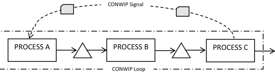
CONWIP loop, the quantity of WIP, jobs being processed plus waiting to be processed, is kept constant. As a job leaves the loop, it triggers a new job to enter the loop as shown in Figure 1.
By limiting the volume/quantity of jobs in the loop, inventory levels are controlled and machines or work cells have a more constant flow of work, thus limiting lead time. Some claim that this is the simplest form of a pull system (Spearman, Woodruff & Hopp, 1990).
Figure 1. Simple CONWIP system
2.2. POLCA
Job movement between any two cells/process in a POLCA system is controled by POLCA cards specific to that loop. The number of cards is the key parameter which limits the WIP inventory. For this reason they are often referred to as capacity signals rather than inventory signals.
Figure 2. Simple Three Loop POLCA system
3. High Mix Low Volume Systems (HMLV)
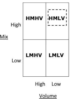
One manufacturing classification, HMLV, refers to production of a variety of products with small order quantity and frequency (the volume), and a high number of differing products (the mix) as shown in Figure 3. This is typical of MTO and/or engineered-to-order (ETO) systems.
Figure 3. Manufacturing Type Matrix
2004). The volatility results in manufacturers needing to supply many different parts types to many different customers, rather than a large volume one part to one customer (Duggan, 2002). As a result, high-mix manufacturers earn business based primarily on how quickly, minimal lead time, they can deliver exactly what their customers want.
Photonics is such an industry. Historically, this industry could be classified as mostly research and development with small prototype orders. Continuing technology evolution has led to more products that include lasers leading to expanding customer bases demanding more product variations.
4. The Case Study Manufacturing System
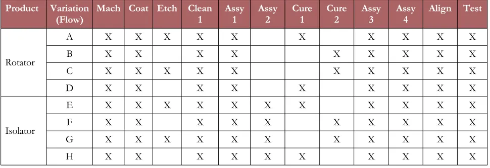
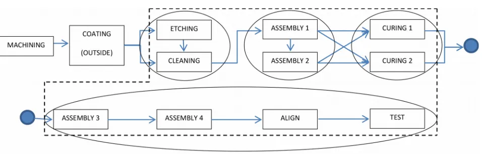
The HMLV system consisted of twelve distinct processes. Two similar products with varying sizes, optical isolators and rotators, will be routed through the system by a process flow that is product and/or customer order predetermined as shown in Table 1.
Product Variation
(Flow) Mach Coat Etch Clean1 Assy1 Assy2 Cure1 Cure2 Assy3 Assy4 Align Test
Rotator
A X X X X X X X X X X
B X X X X X X X X X
C X X X X X X X X X X
D X X X X X X X X X
Isolator
E X X X X X X X X X X X
F X X X X X X X X X X
G X X X X X X X X X X X
H X X X X X X X X X X
Table 1. Product Variations with Corresponding Process Flows/Routings
assembly #2, isolator path, and assembly #1, rotator path, the optics move into either an oven cure, #1, or an ultraviolet cure, #2. From this point both products flow into assembly #3 to have the hubs secured and assembly #4 to have the endcaps secured. All products pass through a final alignment step for adjustment to customer specified settings followed by testing/verification of the entire unit. The base processes and flows of the system are visually depicted in Figure 4.
Figure 4. Base system processes and flows
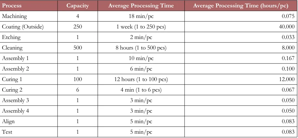
Order arrival rate is defined as the frequency at which customer orders arrive. Time between arrivals, the reciprical of order arrival rate, ranges from once per month to once every six months. Cell capacity is defined as the number of jobs that each process can perform concurrently. Processing time is defined as the value added time the cell takes to transform the units/batches. Cell capacities and processing times are stated in Table 2.
Process Capacity Average Processing Time Average Processing Time (hours/pc)
Machining 4 18 min/pc 0.075
Coating (Outside) 250 1 week (1 to 250 pcs) 40.000
Etching 1 2 min/pc 0.033
Cleaning 500 8 hours (1 to 500 pcs) 8.000
Assembly 1 1 10 min/pc 0.167
Assembly 2 1 6 min/pc 0.100
Curing 1 100 12 hours (1 to 100 pcs) 12.000
Curing 2 6 4 min (1 to 6 pcs) 0.067
Assembly 3 1 3 min/pc 0.050
Assembly 4 1 3 min/pc 0.050
Align 1 5 min/pc 0.083
Test 1 5 min/pc 0.083
Applying Little’s Law from Hopp and Spearman (2011)
WIP = Cycle Time (CT) * Throughput (TH) (1)
the minimum lower bound for the WIP can be determined. Having too little WIP can starve processes, causing interruptions in production flow and lead to long lead times (Standridge, 2013). The cycle time (CT) for each product type is calculated with a summation of the process flow steps in Table 1 with the processing times and capacities in Table 2 and using the average order size, 8. The throughput (TH) for each product type is derived from the average annual order totals from the last three years. Using a summation of Little’s Law for each of the eight different product types and flows yields a lower bound WIP level of 25 batches. This is shown in detail in Table 3.
Product Variation(Flow) (hrs/batch)CT Avg. Annual Volume(8 piece order) (order/hrs)TH WIP = (CT * TH)(batches)
Rotator
A 23.728 532.793 0.266 6.321
B 11.553 59.063 0.030 0.341
C 11.817 667.284 0.334 3.943
D 23.464 108.704 0.054 1.275
Isolator
E 24.528 414.923 0.207 5.089
F 12.353 141.375 0.071 0.873
G 12.617 310.650 0.155 1.960
H 24.264 352.079 0.176 4.271
24.1
Table 3. Minimum WIP Level Calculations
The stations included in the CONWIP control loop are shown with a dashed box in Figure 5. The machining and outside processing (coating) will not be included in the control loop as a product cannot be controlled once it leaves the manufacturing site. Therefore, the CONWIP loop will include all processes post-Coating through Test. The POLCA cells are shown as solid ovals. Thus, the POLCA
system will comprise of three loops: (1) Etch/Clean→Assembly 1_2, (2) Assembly 1_2→Cure 1_2, (3)
Figure 5. CONWIP and POLCA system loops
The sources of variation are the number of orders for each product per year, the number of number of pieces in each order, the manual operating times, and the number of pieces of in each batch operation: shipped to the coating process and processed in the cleaning and curring processes. The latter disrupts flow but can be controlled as a manufacturing operating parameter. For this study, the target number of pieces per batch operation was set to 100 for coating, cleaning, and cure 1 such that the first order that caused the batch to exceed 100 triggers the start of the operation. Cure 2 was allowed to work on one piece at a time. Note also that cleaning and curing 1 are automated processes with long processing times which can be modeled as constants.
5. Simulation Modeling and Experimentation
The goal of the simulation study is to find the minimal WIP level at which a short lead time can be achieved. This can be accomplished by increasing the number of CONWIP and POLCA signal cards starting at the minimum WIP of 25. Note that the number of POLCA cards will exceed the maximum observed WIP as the control areas for individual POLCA card types overlap. Two sets of experiments will be conducted. In the constant case, the order arrival rate, the number of pieces in order (order size with average of 8), and the operation times are treated as constants. In the random case, the number of orders is modeled as Poisson distributed, the order size as uniformly distributed between 1 and 15 pieces, and the operation times as uniformly distributed between 80% and 120% of the average. This approach is consistent with the discuss in Hopp and Spearman (2011) concerning a reasonable range of variability for production systems.
accompany the batch. This approach automatically accommodates the order quantity and is an advantage of a load-based POLCA (LB-POLCA) system (Vandaele, Nieuwenhuyse, Claerhout & Cremmery, 2008).
All orders are processed on an earliest calendar due date basis and treated as though there is not any finished goods inventory from which to fulfill them. The simulation model will ignore the effects of quality rejected materials, scrap, downtime, and WIP rework, which are all minimal.
Simulation run time is 240 production days, one year. This is reasonable considering that the longest time between arrivals for this family of products is typically no longer than six months.
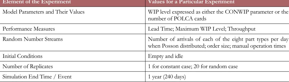
Table 4 summarizes the simulation design of experiments.
Element of the Experiment Values for a Particular Experiment
Model Parameters and Their Values WIP level expressed as either the CONWIP parameter or the number of POLCA cards
Performance Measures Lead Time; Maximum WIP Level; Throughput
Random Number Streams Number of arrivals of each of the eight part types per day
when Posson distributed; order size; manual operation times
Initial Conditions Empty and idle
Number of Replicates 1 for constant case; 20 for random case
Simulation End Time / Event 1 year (240 days)
Table 4. Simulation Experimental Design
5.1. Verification and Validation
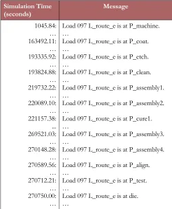
Next model verification and validation are discussed. The techniques used are those discussed in Sargent (2012) specifically tracing entities through all processes as well as the use of simple analytic models such as balance equations and utilization computations. Law (2007) also indentifies tracing entities as a specific verification technique as well as using machine utilization for validation by comparing simulation results to data collected from the actual system.
Process flow for each load type was confirmed by tracing all the processes listed in sequence for both the CONWIP and POLCA models with constant arrivals. Typical results are shown in Table 5 which shows that “Load 97” follows the correct route.
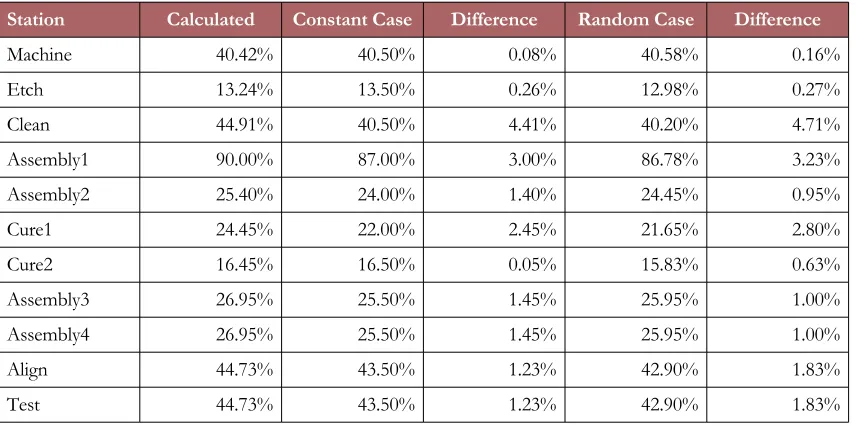
Validation evidence was obtain by comparing the utilization of resources obtained by simulation with utilizations calculated from system data. A simulation of the exising system without the effect of CONWIP or POLCA controls is accomplished by setting the WIP level parameters to a very high number. Simulation experiments were conducted for both the constant and random cases. The results are shown in Tables 6 and 7. All absolute differences no more than 5% of the values calculated from system data except for the clean and cure1 stations for which the absolute difference is about 10% - 11%. Thus, validation evidence is considered to be obtained. Note that many of the operation utilizations are relatively low, less than 50%.
Simulation Time (seconds) Message 1045.84: … 163492.11: … 193335.92: … 193824.88: … 219732.22: … 220089.10: … 221157.38: ... 269521.03: … 270148.28: … 270589.56: … 270712.21: … 270750.00: …
Load 097 L_route_e is at P_machine. …
Load 097 L_route_e is at P_coat. …
Load 097 L_route_e is at P_etch. …
Load 097 L_route_e is at P_clean. …
Load 097 L_route_e is at P_assembly1. …
Load 097 L_route_e is at P_assembly2. …
Load 097 L_route_e is at P_cure1. …
Load 097 L_route_e is at P_assembly3. …
Load 097 L_route_e is at P_assembly4. …
Load 097 L_route_e is at P_align. …
Load 097 L_route_e is at P_test. …
Load 097 L_route_e is at die. …
Station Calculated Constant Case Difference Random Case Difference
Machine 40.42% 40.50% 0.08% 40.58% 0.16%
Etch 13.24% 13.50% 0.26% 12.98% 0.27%
Clean 44.91% 40.50% 4.41% 40.20% 4.71%
Assembly1 90.00% 87.00% 3.00% 86.78% 3.23%
Assembly2 25.40% 24.00% 1.40% 24.45% 0.95%
Cure1 24.45% 22.00% 2.45% 21.65% 2.80%
Cure2 16.45% 16.50% 0.05% 15.83% 0.63%
Assembly3 26.95% 25.50% 1.45% 25.95% 1.00%
Assembly4 26.95% 25.50% 1.45% 25.95% 1.00%
Align 44.73% 43.50% 1.23% 42.90% 1.83%
Test 44.73% 43.50% 1.23% 42.90% 1.83%
Table 6. Individual Resource Utilization Comparison and Validation For CONWIP model
Station Calculated Constant Case Difference Random Case Difference
Machine 40.42% 40.50% 0.08% 40.58% 0.16%
Etch 13.24% 13.50% 0.26% 12.98% 0.27%
Clean 44.91% 40.50% 4.41% 40.20% 4.71%
Assembly1 90.00% 87.00% 3.00% 86.78% 3.23%
Assembly2 25.40% 24.00% 1.40% 24.45% 0.95%
Cure1 24.45% 22.00% 2.45% 21.65% 2.80%
Cure2 16.45% 16.50% 0.05% 15.83% 0.63%
Assembly3 26.95% 25.50% 1.45% 25.95% 1.00%
Assembly4 26.95% 25.50% 1.45% 25.95% 1.00%
Align 44.73% 43.50% 1.23% 42.90% 1.83%
Test 44.73% 43.50% 1.23% 42.90% 1.83%
Table 7. Individual Resource Utilization Comparison and Validation For POLCA model
6. Results and Comparisons
Simulation results are presented for each WIP control system. Conclusions are drawn by comparing the results.
6.1. CONWIP Results
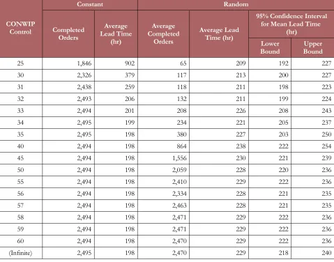
work-in-process is unconstrained (a CONWIP parameter of infinite). The lead time continues to decrease as the CONWIP parameter value increases reaching only 3 hours more than for unconstrained WIP for a CONWIP parameter value of 33 and within 1 hour for a CONWIP parameter value of 34.
Now consider the results for the random case. The number of orders processed becomes equivalent at a CONWIP parameter value of 57 to those processed when the work-in-process is unconstrained with lead time also equivalent to that achieved when the work-in-process in not constrained.
CONWIP Control Constant Random Completed Orders Average Lead Time (hr) Average Completed Orders Average Lead Time (hr)
95% Confidence Interval for Mean Lead Time
(hr) Lower
Bound BoundUpper
25 1,846 902 65 209 192 227
30 2,326 379 117 213 200 227
31 2,438 259 118 211 198 223
32 2,493 206 132 211 199 224
33 2,494 201 208 226 208 243
34 2,495 199 234 221 205 237
35 2,495 198 380 227 203 250
40 2,494 198 864 238 222 254
45 2,494 198 1,556 230 221 239
50 2,494 198 2,059 228 220 236
55 2,494 198 2,410 229 222 236
56 2,494 198 2,334 228 221 235
57 2,494 198 2,463 228 221 235
58 2,494 198 2,471 229 222 236
59 2,494 198 2,471 229 222 236
60 2,494 198 2,470 229 222 236
(Infinite) 2,495 198 2,470 229 218 240
Table 8. CONWIP Parameter Control Simulation Results
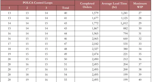
6.2. POLCA Results
9 shows the combinations yielding the shortest lead time for each maximum WIP level from 27 through 40. Recall that the maximum WIP level is less than the number of POLCA cards due to the overlapping loops.
The throughput becomes equivalent to the unconstrained WIP case (infinite) shown in Table 8 for a maximum WIP value of 36. Lead time continues to decrease through a maximum WIP of 39.
POLCA Control Loops Completed
Orders Average Lead Time(hr) MaximumWIP
1 2 3 Total
13 13 14 40 1,579 1,241 27
13 14 14 41 1,677 1,125 28
14 14 15 43 1,772 1,,012 29
15 14 14 43 1,867 882 30
16 14 14 44 1,965 794 31
16 15 15 46 2,065 660 32
17 15 15 47 2,182 535 33
18 15 15 48 2,327 380 34
19 15 15 49 2,474 221 35
20 15 15 50 2,490 212 36
20 16 15 51 2,493 204 37
20 17 16 53 2,495 200 38
20 18 16 54 2,495 199 39
20 19 16 55 2,495 199 40
Table 9. POLCA Parameter Control Simulation Results – Constant Case
POLCA Control Loops
Completed Orders
Average Lead Time
(hr)
95% Confidence Interval for Mean Lead Time
(hr) Max WIP
1 2 3 Total BoundLower BoundUpper
35 26 27 88 969 213 189 238 60
35 28 29 92 1,239 214 189 238 61
35 29 29 93 1,420 215 190 239 62
35 30 28 93 1,175 213 189 238 63
40 41 41 122 2,056 229 222 237 68
41 43 40 124 2,086 230 223 238 69
41 42 43 126 2,063 229 222 236 70
43 41 45 129 2,371 229 222 235 71
43 41 40 124 2,462 230 223 236 72
43 44 41 128 2,481 230 222 239 73
45 40 40 125 2,504 230 223 238 74
45 41 40 126 2,505 230 223 238 75
Table 10. POLCA Control Simulation Results – Random Case
6.3. Comparison
The following can be concluded from the simulation results shown in Tables 8, 9, and 10. The results are consistent with those reported by Germs and Riezebos (2010).
First consider the constant case. As seen in Table 8, a CONWIP control level of 32 results in a number of completed orders equivalent to an infinite WIP control level that is no WIP control. As seen in Table 9, an equivalent number of completed orders is achieved for a control level of 50 total POLCA cards and a maximum WIP of 36. The lead times for the two control strategies are equivalent for the above control levels. There is no random variation. Thus, it can be concluded that the higher number of POLCA cards and maximum WIP versus CONWIP to achieve an equivalent number of completed orders (throughput) has do with the differences in order flow caused by the two control strategies. With CONWIP, there is no constraint of order flow from station to station. With POLCA, a card must be obtained to enter each loop which constrains order flow. For this system, the constrained flow requires a high level of maximum WIP to achieve the same throughput with the same lead time. On the other hand for some systems, POLCA can present orders from collecting in one part of the system only and blocking flow, while CONWIP cannot. It appears that CONWIP performs better for this case due to batch operations and the relatively low utilization of the manual operations.
has little impact. The squared coefficient of variation associated with the number of orders is one by definition of the Poisson distribution. The squared coefficient of variation of the manual processing times is 0.013, two orders of magnitude less. With order sizes ranging from 1 to 15 pieces, the number of order per batch for cleaning and curing operations is highly variable as well. Hopp and Spearman (2011) discuss how lead time is proportional to the squared coefficient of variations of the number of orders and of processing times.
Thus, it is not surprising that the CONWIP level needed to achieve an equivalent number of completed orders to those achieved with no WIP control rises from 32 in the constant case to 57 in the random case as shown in Table 8. Lead time rises by about 10% with a narrow 95% confidence interval for the true mean lead time, a half-width of 3%-4% of the average.
In the same way, the POLCA cards needed to achieve an equivalent number of completed orders to those achieved with no WIP control more than doubles from 50 in the constant case to 128 in the random case with the average maximum WIP doubling from 36 to 73 as seen in Tables 9 and 10. The average lead time is about the same as for the CONWIP case and also has a narrow confidence interval half-width.
7. Summary
In summary, this case study focused on two strategies, CONWIP and POLCA, for controlling WIP in a HMLV, photonics industry manufacturing environment with 12 products and batch operations using lead time, maximum WIP, and throughput as the primary performance measures. A discrete event simulation model and experiment were employed.
Based on the simulation results, it can be concluded that the CONWIP control performs better than the POLCA control for this system. The CONWIP control achieves maximum throughput at a lower maximum WIP level than POLCA for both the constant and random cases. The average lead times for CONWIP and POLCA for the maximum throughput level are equivalent in both the constant and random cases. Any issues with WIP gathering in one area of the system, which POLCA could prevent but CONWIP cannot, were not encountered in this system likely due to the batch operations and relatively low utilizations of the manual operations.
References
Duggan, K.J. (2002). Creating Mixed Model Value Streams: Practical Techniques for Building to Demand. New York, NY: Productivity Press.
Germs, R., & Riezebos, J. (2010). Workload balancing capability of pull systems in MTO production. International Journal of Production Research, 48(8), 2345-2360. http://dx.doi.org/10.1080/00207540902814314
Godinho-Filho, M., & Saes, E.V. (2013). From time based competition (TBC) to Quick Response Manufacturing (QRM): the evoluation of research aimed at lead time reduction. International Journal of Advanced Manufacturing Technology, 64, 1177-1191. http://dx.doi.org/10.1007/s00170-012-4064-9
Hopp, W., & Spearman, M. (2011). Factory Physics. 3rd ed. Waveland Press.
Kabadurmus, O. (2009). A comparative study of POLCA and generic CONWIP production control systems in erratic demand conditions. IIE Annual Conference.Proceedings. 1197-1202. Available at:
http://search.proquest.com.ezproxy.gvsu.edu/docview/192457092?accountid=39473
Kishnamurthy, A., & Suri, R. (2000). A New Approach for Analyzing Queuing Models of Material Control Strategies in Manufacturing Systems. Center for Quick Response Manufacturing, University of Wisconsin-Madison, Madison, WI.
Law, A.M. (2007). Simulation Modeling & Analysis. 4th ed. New York: McGraw-Hill.
Sakhardande, R. (2011). A performance comparison between kanban and CONWIP through simulation. IIE Annual Conference Proceedings. 1-8. Available at:
http://search.proquest.com.ezproxy.gvsu.edu/docview/1190330695?accountid=39473
Sargent, R.G. (2012). Verification and validation of simulation models. Journal of Simulation, 7, 12-24.
http://dx.doi.org/10.1057/jos.2012.20
Spearman, M.L., Woodruff, D.L., & Hopp, W.J. (1990). CONWIP: A pull alternative to kanban. International Journal of Production Research, 28(5), 879-894. http://dx.doi.org/10.1080/00207549008942761
Sprovieri, J. (2004). Managing high-mix, low-volume assembly. Assembly Magazine, Available at:
http://www.assemblymag.com/articles/83764-managing-high-mix-low-volume-assembly (accessed April 2016)
Standridge, C.R. (2013). Beyond Lean: Simulation in Practice. 2nd ed. Available at:
http://scholarworks.gvsu.edu/books/6/(Accessed: April 2013).
Vandaele, N., Nieuwenhuyse, I.V., Claerhout, D., & Cremmery, R. (2008). Load-Based POLCA: An Integrated Material Control System for Multiproduct, Multimachine Job Shops. INFORMS. Manufacturing & Service Operations Management, 10(2), 181-197. http://dx.doi.org/10.1287/msom.1070.0174
Journal of Industrial Engineering and Management, 2016 (www.jiem.org)
Article's contents are provided on an Attribution-Non Commercial 3.0 Creative commons license. Readers are allowed to copy, distribute and communicate article's contents, provided the author's and Journal of Industrial Engineering and Management's