Price and Volume Effects Associated with Index
Additions: Evidence from the Indian Stock Market
Srikanth Parthasarathy
Research Scholar, Loyola Institute of Business Administration University of Madras (Chennai)
Loyola College, Nungambakkam, Chennai-34, India Tel: 91 – 909-413-5843 E-mail: psrikanth2011@gmail.com
Received: 2010-09-16 Accepted: 2011-05-18 doi:10.5296/ajfa.v2i2.469
Abstract
This study investigates the price and volume effect of index additions to the benchmark Nifty index for the recent period 1999-2010 in the Indian stock market. This study evidences significant, positive permanent abnormal returns around index announcement and inclusion. The support for permanent abnormal volume around index additions is limited at best. The results in this study do not support either the downward sloping demand curve hypothesis or the price pressure hypothesis as the primary explanation for the index inclusion effect. This study contributes to the growing literature on index inclusion by providing evidence that stock addition to the benchmark Nifty index appears to convey information.
Keywords:Indian Equity market, Nifty index additions, Abnormal return and volume,
Introduction
In the past decades, numerous studies have documented the ‘index effects’ associated with stock index changes predominantly in the developed markets. The included stocks experience a significant increase in prices after the announcement and further rise around the actual inclusion. Though some of the gain is lost after inclusion, a permanent increase in return is predominantly evidenced over a period of time. Trading volumes also increase significantly around announcement and inclusion in the developed markets. The findings are not consistent with market efficiency as index changes are made with apparently made with readily available public information, the slow multiple day price adjustments and volume effects around the stock index changes directly questions the validity of semi-strong efficiency which requires all publicly available information to be reflected in the stock prices quickly.
Researchers have forwarded various hypotheses to explain the index effects. They are broadly classified into two groups based on their assumption of information content. The first group assumes that the index changes does not convey any information and have attributed the change in price to non-flat demand curve rather than change in fundamental value. In an ideal Capital Asset Pricing Model (CAPM) world, stock prices depend on the return – risk characteristics. In an information free event, the demand curve will be horizontal as the investors can alter their portfolio using near-perfect substitutes to reflect their return-risk profile. If perfect substitutes are not available, then a shock leads to a permanent stock price change as investors expect compensation in order to rebalance their portfolios. An index changes creates excess demand which cannot be satisfied without a shift in the demand curve as stocks are not perfect substitutes (Shiefler, 1986). Hence the abnormal returns around the inclusions are explained by the changes in the aggregate demand of the stocks due to lack of perfect substitutability and hence downward sloping demand curve. Price pressure hypothesis (Harris and Gurel, 1986) too assumes lack of information in index changes and posits downward sloping demand curve but only in the short term. According to this hypothesis, excess demand due to the indexing and institutional investor activity creates price pressure and reverses once the temporary excess demand is satisfied.
The second group of explanations assumes that index changes convey information about the stocks. The index inclusion has an impact on the fundamental value of the stock thereby in the present value of the discounted cash flow. This can work through two ways, namely the expected cash flow or the discount rate. The explanations for increase in cash flow may be the certification hypothesis supported by Dhillon and Johnson (1991), Jain(1987), in which
the stocks inclusion to the Nifty index may convey positive information regarding the future prospects of the company. Denis et al. (2003) and Chen et al (2004) support the Investor awareness hypothesis which postulates that following index inclusions, investors change the
expectation of future cash flow of the stocks as the firms perform better due to enhanced monitoring by analysts and investors.
The explanations for decrease in the discount rate are liquidity hypothesis, (Amihud and
index stocks causes greater information production. This induces a reduction in the information asymmetry and causes increased liquidity. If some investors know only a subset of stocks and trade only those stocks then those investors will require a premium called the ‘shadow cost’ for the non-systematic risk (Merton,1987).
There are few studies in the emerging markets like India on index changes. The importance of these studies in the Indian stock market can be appreciated based on the fact that the Indian equity market stood 13th in the world and 4th in Asia in terms of both traded value ($ 1050 bn
during 2008) and market capitalisation ($ 645 bn at the year end)1 in 2008. The increasing international portfolio investment and participation provides a perfect platform for gathering information about the market structure, efficiency and evidence of the integration mechanism with the developed markets.
The Indian stock market differs from the developed markets in the following ways; the Indian stock market1 is characterized by less informational efficiency, higher costs, smaller investor base and lower liquidity compared with the stock markets of developed countries. Finally, unlike the developed markets, there may be drastic difference in the quality of assets between benchmark index and other index stocks. This is truer for the foreign investors’ as local factors affect pricing significantly.
This study attempts to enter the debate by studying index inclusion effect in the Nifty index, premier benchmark index in the Indian stock market by focusing on the abnormal return, volume and liquidity around two event dates namely ‘announcement date’(AD) and the ’Effective date’(ED).
The purpose of this study is twofold: whether abnormal returns are permanent and whether Nifty index changes convey information. This study expects index addition to cause significant permanent abnormal return for the added stocks and enters the debate by positing that the information explanation might explain the index inclusions better in emerging market like India. This study makes two contributions to the growing index inclusion literature. First, it tests the Nifty index additions, premier index of the Indian stock market in the current period. Also very few papers have focused on the information aspect in the emerging markets.
The second section details the theoretical explanations and literature review for the index inclusion effect. The third section details the ‘Nifty’ index selection process and methodology. The fourth section gives the findings and analysis and the fifth section concludes.
2. Review of Literature
The literature analyzing the price and volume effects of index changes is ever growing. The existing literature is grouped as per the explanations with the studies supporting information free hypothesis given first. Shiefler (1986) studying changes to the S&P 500 index for the period 1976-1983 documented a permanent 2.37% abnormal return and suggested DSDC
hypothesis as the reason. Lynch and Mendenhall (1997) studying S&P 500 changes for the period 1990-1995 documents significant abnormal return subsequent to the announcement. They evidenced part reversal consistent with both price pressure and DSDC hypothesis. Wurgler and Zhuravskaya (2002) based on the difficulty to arbitrage in the absence of perfect substitutes examined the announcement returns relative to a arbitrage measure and found support for DSDC hypothesis.
Harris and Gurel (1986) studying S&P 500 index additions for the period 1976-1983 documented 3.13% abnormal return and found a systematic reversal of initial abnormal return in support of price pressure hypothesis. Elliot and Warr (2003) also find support for price pressure but only around the inclusion date. Mase (2002) studying FTSE 100 inclusion effects for the period 1992 – 1999 find support for the price pressure hypothesis. Studies have generally supported partial price pressure in the developed markets.
There are studies supporting information – free assumption on the index addition induced comovement2 between the return of the included stocks and the index. Vijh (1994) evidences significant comovement for S&P 500 additions and supports index fund trading as major cause. Barberis, Shliefer and Wurgler (2005) differentiate between the traditional view of frictionless markets3 and non frictionless markets. In a frictionless market comovement in stocks implies comovement in the fundamentals and the prices may reflect the information more quickly compared to other stocks. In a non frictionless market, comovement between added stocks may be due to category based trading and habitat based trading supporting the information-free assumption. They have suggested that for the friction based comovement, beta of the added stocks would be stronger in the latest data with the increase in institutional investor activity.
The evidence in favour of the information explanations are, Dhillon and Johnson(1991), Jain(1987) studying the inclusion effects of S&P 500 found evidence for the certification hypothesis. Denis et al. (2003) postulate that following index inclusions, investors change the expectation of future cash flow of the stocks as the firms perform better due to enhanced monitoring by analysts and investors. Chen et al (2004) examined the S&P 500 index changes for the period 1976 – 2000. He concludes that investor awareness is the primary reason for the S&P 500 index inclusion effect and greater interest for the index stocks induces a reduction in information asymmetry due to increased information production which results in increased liquidity. Bhenish and Whaley (1996) studying S&P 500 inclusions for the period 1986-1994 evidence increased trading volume. Hradzil (2009) studying S&P 500 stocks find little evidence for the DSDC hypothesis and finds support for the liquidity and information hypothesis. Some of the recent researches in the developed markets seem to support investor awareness hypothesis. Burcu Hadicebel (2008) and Chakrabarti (2002) studying the inclusion of stocks from the emerging markets to the global MSCI index evidence permanent increase in price and volume and that index inclusion convey information. Kumar (2005) studying
2 Barberis et al(2002) defines comovement as a pattern of positive correlation. In this study comovement of stock return of the included stock and the index return is discussed.
Nifty index additions in the Indian stock market for the period 1998 - 2003 did not find any significant index effects around announcement dateand evidenced 1.47% effective date (ED) abnormal return. Li and Sadeghi (2009) analysed the Chinese index additions have evidenced permanent abnormal returns and increased liquidity post inclusion. They have also found support for information based explanations for the index additions in the Chinese stock market.
3. Data and Back Ground Information
3.1 The Nifty information
The S&P CNX nifty (Nifty hereafter) is the headline index on the National stock exchange (NSE) maintained by the India index services and products Ltd.(IISL) since the year 1996. Previously the index was managed by CRISIL. It represents a portfolio of 50 large and most liquid stocks of the NSE and captures nearly 65% of the total market capitalization as on December 2009. The main criteria of selection of stocks for the Nifty index are market capitalization, float, liquidity and industry representation. The index is normally reviewed every six months and six weeks’ notice is normally given to the market before the change is effected. Index removal is normally effected due to corporate actions like restructuring etc. and when market capitalisation of an index stock falls below 50% of the market capitalisation of the top most stock of the replacement pool.
3.2 Sample selection:
The sample period for this study is 1999 - 2010 to coincide for the start of index funds in India. The details regarding both announcement date (AD) and Effective date (ED) are available only from 1998. The daily data from www.nse-india.com is used to calculate daily
return and daily volume of the added stocks and Nifty index.
Appendix 3 displays the frequency of trading days between index addition announcement date (AD) and the index inclusion date (ED) for the stocks included in the Nifty index between 1999- 2010.
The following stocks are not considered. A) Stocks arising out of corporate restructuring are not considered. B) Stocks which do not have trading history for at least six months prior to the announcement date. C) Stocks which do not have at least 5 clear trading days between announcement and effective date are not considered.
The total Nifty index additions are 54 for the 1999-2010 period. The total number of stocks available for research after the elimination is 38. Appendix 1 lists all the included stocks available for research. Even though the sample is small, it comprehensively covers the recent 11 year period in the Indian stock market. The sample is separated into two periods namely, 1999 - 2006 and 2007 – 2010. The latter period is marked by increased institutional activity and participation and represents the current market activity.
3.3 Abnormal returns
announcement date (AD) and effective date (ED). The daily abnormal returns are calculated as the stocks excess return on day ‘t’ over the index return as in Lynch and Mendenhall(1998) wherein it is observed that more sophisticated models of abnormal return generation like single factor market model gives very similar results to the simple abnormal return of the stock over the index return. This study uses both cumulative abnormal return (CAR) and average abnormal return (AAR). AAR aggregated over the event window gives the CAR. Conversely, The CAR divided by the number of days in the event window gives the AAR. The CAR of a stock represents the ‘buy and hold’ return over the specific period as buy and hold returns are more relevant to the investors. The CAR of all the sample stocks are aggregated and averaged over the event window to calculate the overall CAR for the entire sample.
Daily return Rt is calculated as
Rt = Ln ( Pt ) - Ln (Pt-1) (1)
Where Pt is the stock / nifty closing price at time t and Pt-1 is the stock / nifty closing price at
time t-1.
Abnormal Return (ARit) = Rit - Rmt, (2)
Where Rit is the stock return and Rmt is the Nifty index return on day ‘t’.
3.4 Abnormal volume
The volume effect is studied in the spirit of Harris and Gurel(1986) where
Volume Ratio VR = (Vit /Vmt) ÷ (Vi / Vm) (3)
Where Vit and Vmt are the trading volumes of security I and the total NSE respectively, and Vi
andVm are the average trading volumes of the security I and total NSE for the period AD-70
through AD-10. The daily VR is averaged across the various event windows. The volume ratio4 should have a value of ‘one’ under null hypothesis. If in any event window VR is significantly greater than one then volume is said to be abnormal for that event window.
3.5 Liquidity Ratio
Amihud(2002) liquidity measure is used.
Liquidity Ratio = VOLit / │Rit │ ÷ VOLi / │ Ri │ (4)
Where VOLit is the daily rupee volume and Rit is the daily stock return. ‘VOLi / │ Ri │’isthe
average liquidity of the security I for the period AD-70 through AD-10. If in any event window the average liquidity ratio is significantly greater than one then liquidity is said to be abnormal for that event window.
3.6 The Event and Event Windows
In this study, the Nifty index inclusions between 1999 -2010 are analyzed. The two important event dates are announcement date (AD or day ‘0’) and the effective date of inclusion(ED). The actual AD is the day following the announcement date (AD+1 or Day ‘1’) as normally announcements regarding inclusion are made after trading hours and consequently the effects are reflected the next day of the announcement Unlike the US market, the number of days between AD and ED varies between 5 to 31 trading days (mean is approximately 25 trading days, median is 27 days). In order to avoid the effect of other events vitiating the study of inclusion effects, the total event window starts 10 days before AD and ends 60 days after inclusion.
The event windows are
1. Anticipation window runs through AD-10 to AD. 2. AD window5 includes AD+1, AD+2, AD+3.
3. Run up window covers the period AD+4 to ED-1. 4. ED is the actual inclusion date.
5. Release window which runs from ED+1 to release ending day (Lynch and Mendenhall, 1997).
6. ED long run window running from ED to ED+60
7. Finally, the long term effect window is studied between ED+30 to ED+60.
According to Lynch and Mendenhall (1997), the release ending day is the day when the demand for the stocks reach the normal post change level ( ie. When the index demand ends and price release starts (price pressure ends)). The volume is estimated to have returned to the normal post inclusion level on the earliest day after the change day when the mean abnormal volume is lower than the average mean abnormal volume for all the days from that day through to ED +10.
Similar to other studies ‘price pressure hypothesis’ is analysed around ED as the index funds rebalance their portfolio around ED to avoid tracking error6. All the other explanations are studied around AD (Lynch and Mendenhall, 1997).
3.7 Regressions
Firstly, regression with dummy variables7 is used to distinguish between the event days AD+1 abnormal return and ED abnormal return separately with that of other days.
Yi= β0 + β1 *Zi + ε (5)
where, Zi is ‘1’ if AD+1 or ED and ‘0’ otherwise. β1 measures the difference in the
5 The rationale behind the choice of AD window as AD+1,AD+2,AD+3 is based on the criterion that both mean
and median VR is greater than ‘1’. Also for the AD window the number of stocks for which CAR >0 is more than 50%. Neither AD nor AD+4 satisfies the above criterion
abnormal return between the event days and other days.
Secondly, the cross sectional regressions in the spirit of Shliefer(1986) who regressed the day ‘1’ AD window abnormal return (ABRET CAR) and abnormal volume (ABVOL) to examine the relationship between abnormal return and abnormal volume as a significant slope co-efficient is consistent with downward sloping curves for the added stocks.
AD window ABRET CAR = α + ψ * AD ABVOL (6)
AD window ABRET CAR = α + ψ * AD ABVOL + µ * USVOL (7)
where, ABRET is the abnormal return, ABVOL is the abnormal volume and USVOL is the usual volume( Average VR from AD-10 to AD-1).
Another regression for examining the co-movement of the added stocks
Rit = α + β * Rmt + εit (8)
where, Rit is stock return, Rmt is the Nifty index return on day ‘t’ and εit is a random variable
with expected value of zero and assumed to be uncorrelated with Rmt. The daily pre-event
regression is run for the period AD-70 to AD-10. The daily post event regression is run for ED+10 to ED+70. The focus of interest is the difference βc which is calculated for each added
stock by subtracting the pre- event beta from the post event beta.
4. Findings and Analysis
4.1 Analysis of Abnormal return
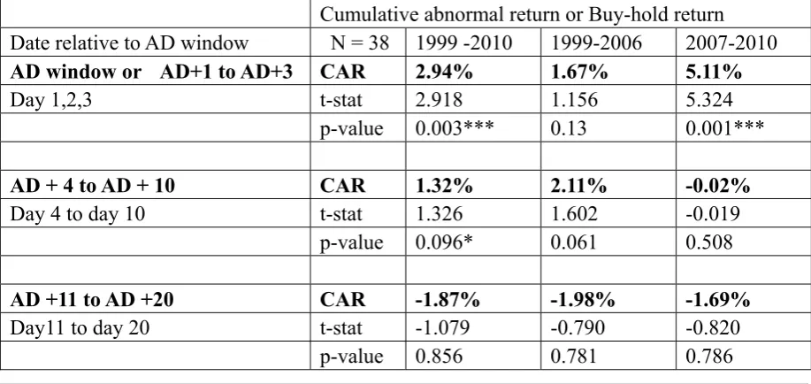
The abnormal return surrounding the event day AD is analysed in this section. Table 1 presents the results of the event study during AD window and subsequent to AD window (excluding AD window) to test for reversion in the near term. It is seen that for the complete period 1999-2010, there is a 2.94% AD announcement return which is not only statistically significant at 1% level but also economically significant. The results for Nifty inclusions for the period 1999 - 2010 in this regard are comparable to the developed markets in general and S&P 500 in particular. The AD window abnormal return for the sub-period 1999-2006 is 1.67% and for the sub-period 2007-2010, a statistically and also economically8 highly significant 5.11%. Table 1 reports the share price behavior subsequent to the AD window.
Table 1 - Test of permanent abnormal return subsequent to announcement of addition to Nifty index for the period 1999-2010.
Cumulative abnormal return or Buy-hold return
Date relative to AD window N = 38 1999 -2010 1999-2006 2007-2010
AD window or AD+1 to AD+3 CAR 2.94% 1.67% 5.11%
Day 1,2,3 t-stat 2.918 1.156 5.324
p-value 0.003*** 0.13 0.001***
AD + 4 to AD + 10 CAR 1.32% 2.11% -0.02%
Day 4 to day 10 t-stat 1.326 1.602 -0.019
p-value 0.096* 0.061 0.508
AD +11 to AD +20 CAR -1.87% -1.98% -1.69%
Day11 to day 20 t-stat -1.079 -0.790 -0.820
p-value 0.856 0.781 0.786
The sample includes all the Nifty additions for the period 1999-2010 in the Indian stock market. ‘AD’ is the announcement day. ‘ED’ is the actual date of inclusion. The cumulative abnormal return(CAR) measures the buy and hold returns for AD window and starting from the day after AD window to the dates mentioned.
*, **, *** indicate significance that the observed mean is significantly greater than zero (one tailed t-test) at 10%, 5%, 1% level respectively.
For the complete period, the cumulative abnormal return (CAR) for the periods AD + 3 to AD + 10 and AD+11 to AD+20 is 1.32% and -1.87% respectively. The negative CAR’s subsequent to AD is not only small but also statistically not significant for the complete period and sub-periods. The results shows that share prices do not fall significantly even after 20 days after AD. Interestingly, it is seen that the overall CAR from AD+1 through AD+10 is 3.78% for the first sub-period and 5.09% for the second sub-period.
The lower AD effect in the first period is somewhat compensated in the AD+3 to AD+10 window. However for the second sub-period the highly significant 5.11% abnormal return during AD window is followed by -0.02% in the AD+3 to AD+10 window. It appears that ‘AD effect’ took longer to take effect in the first sub period than in the recent sub-period (2007-2010).
Table 2. Test of permanent abnormal return subsequent to AD. CAR measures the buy and hold return from AD+1 or Day’0’ to the indicated day.
Including AD window Cumulative abnormal return or Buy-hold return
Period 1999 -2010 1999-2006 2007-2010
AD window or AD+1 to AD+3 CAR 2.94% 1.67% 5.11%
Day1,2,3 t-stat 2.918 1.156 5.324
N=38 p-value 0.003*** 0.13 0.001***
AD+1 to AD + 30 CAR 4.70% 5.13% 4.01%
Day 1 to day 30 t-stat 2.271 1.681 1.793
p-value 0.015** 0.053* 0.048**
AD+1 to AD + 60 CAR 4.63% 3.77% 6.09%
Day 1 to day 60 t-stat 1.316 0.786 1.207
p-value 0.098* 0.220 0.123*
AD+1 to AD + 70 CAR 7.01% 6.62% 7.55%
Day 1 to day 70 t-stat 1.782 1.210 1.486
p-value 0.041** 0.114 0.085*
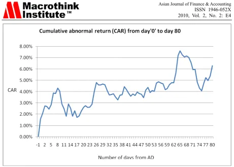
Figure 1. The mean cumulative abnormal return of the stocks included in the Nifty index between 1999-2010.This represents the buy and hold return from day 0 to day T. The x-axis
represents the mean CAR and the y-axis represents the number of days from AD.
The results in Table 1 and Table 2 support the permanent nature of the AD price effects following Nifty additions. Shiefler (1986) points out that as one moves from AD, the standard error of the cumulative return rises. Consequently though the cumulative abnormal return continues to rise and remains economically very significant (see figure-1), it is not statistically significant in a few cases. Hence it can be concluded that the abnormal returns are permanent, increasing and statistically significant even after 70 days from AD for Nifty inclusions between 1999 and 2010. Similar conclusion can be made for the both the sub periods with the recent sub-period displaying increased index addition effect. As the Indian stock market becomes broad based, it appears that AD effect becomes more prominent. The above results evidencing permanent abnormal return following AD are similar to many studies in the developed markets and emerging markets.
4.2 Event windows
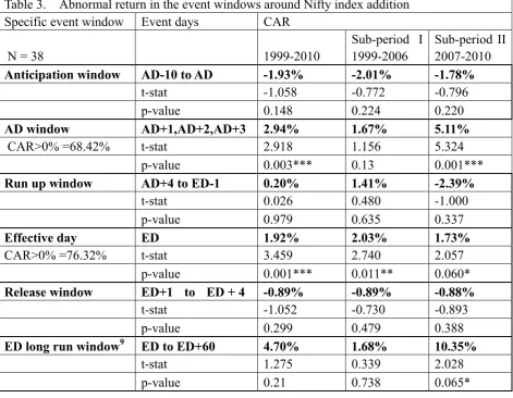
The results for the event windows are tabulated in Table 3. A significantly positive CAR for the anticipation window will imply anticipation and leakage of index change announcements. However the anticipation window CAR is negative (-1.93%) suggesting no evidence of anticipation prior to the announcement for the complete period 1999 – 2010. The results for both the sub-periods are also negative and statistically not significant.
2007-2010 period is 1.41% and -2.39% respectively and both are not statistically significant. According to Lynch and Mendenhall(1987), positive and significant run-up CAR is consistent with the DSDC hypothesis. The results from this study show that the run-up CAR is not statistically significant. Further, for the recent second sub period the run-up CAR is negative as against the requirement of significantly positive run-up CAR for DSDC hypothesis. The overall results in general and the recent period results in particular evidence strongly against the DSDC hypothesis.
Table 3. Abnormal return in the event windows around Nifty index addition
Specific event window Event days CAR
N = 38 1999-2010
Sub-period I 1999-2006
Sub-period II 2007-2010
Anticipation window AD-10 to AD -1.93% -2.01% -1.78%
t-stat -1.058 -0.772 -0.796
p-value 0.148 0.224 0.220
AD window AD+1,AD+2,AD+3 2.94% 1.67% 5.11%
CAR>0% =68.42% t-stat 2.918 1.156 5.324
p-value 0.003*** 0.13 0.001***
Run up window AD+4 to ED-1 0.20% 1.41% -2.39%
t-stat 0.026 0.480 -1.000
p-value 0.979 0.635 0.337
Effective day ED 1.92% 2.03% 1.73%
CAR>0% =76.32% t-stat 3.459 2.740 2.057
p-value 0.001*** 0.011** 0.060*
Release window ED+1 to ED + 4 -0.89% -0.89% -0.88%
t-stat -1.052 -0.730 -0.893
p-value 0.299 0.479 0.388
ED long run window9 ED to ED+60 4.70% 1.68% 10.35%
t-stat 1.275 0.339 2.028
p-value 0.21 0.738 0.065*
The sample includes all the Nifty additions for the period 1999-2010 in the Indian stock market. ‘AD’ is the announcement day. ‘ED’ is the actual date of inclusion. - Cumulative Abnormal Returns in smaller event windows -1999 -2010. The first column specifies the event window of interest. The actual start end dates are specified in the second column. The cumulative abnormal return(CAR) for complete period, first and second period in columns 3,4 and 5 respectively.*, **, *** indicate significance at 1%, 5% and 10% level respectively.
In the ED window, it is observed that CAR for the complete period as well as the sub-periods is statistically and economically significant. It is 1.92% for the complete window, 2.03% for
the first sub-period and 1.73% for the second sub-period. While the ED window CAR is significant at 1% level for the complete period, the ED window for the first and second period is significant at 5% level and 10% level respectively. The percentage of stocks with positive CAR is 76.32%. The inclusion day abnormal return is supposed to be positive due to the action of index funds. This assertion is supported by high percentage of stocks with positive CAR during ED, even higher than on AD. A control mean including only the stocks with positive CAR was calculated. It is statistically and economically significant 3.18% for the whole period, 3.26 for the first period and 3.06 for the second period.
The release ending day is relevant to the ‘Price pressure hypotheses’. The release ending day is ED+4 based on the median values. The abnormal return for the complete period is -0.89%. It is -0.89% and -0.88% for the first and second sub-period respectively. The abnormal returns are not statistically significant.
The results for the long run ED window suggests that the post ED returns are increasing and economically significant for the complete period and the second sub period. Even for the first sub period, the post ED returns is positive though not statistically significant. The results for the AD window and the ED are similar to the index additions in the developed markets. However the absence of significant ‘release window’ CAR and the lack of significant run-up CAR in the Nifty index additions are not consistent with the results in the developed markets. The significant negative anticipation window CAR is very interesting in the light of Li and Sagedhi(2009) in the emerging Chinese stock market. They have evidenced significant negative CAR during the ‘AD-120 to AD’ period in the Chinese market followed by significant CAR post announcement. They have attributed the results to ‘informed syndicate’ traders sending wrong signal to uninformed investors to sell the shares prior to announcement causing the price to fall. However, the index inclusion announcement signals the uninformed investors to buy the shares enabling the informed syndicate traders to reap a huge profit.
In order to test for the above Chinese stock market phenomenon in the Indian stock market, ‘AD-70 – AD-10’ CAR for all the 38 Nifty additions were studied. The Nifty index additions witnessed significant negative CAR of -4.32% during the ‘AD-70 – AD-10’ period followed by significant post announcement CARs in all the tested periods (Table 2). On further examination it is seen that the ‘AD-70 – AD-10’ CAR rises to -1.09%, which is not significant at any level of significance, if one excludes the Nifty additions (numbering 4) during the recession year 200810. Hence it seems that Li and Sagedhi (2009) assertion in the Chinese markets is not supported in the Indian stock market.
4.3 Abnormal Volume
The results in Table 4 suggest that even though the mean VR for the various event windows are significant, the median values and the percentage of stocks with VR>1 in each event
window suggests that the outliers in the higher side have skewed the results. In fact except for the AD window and ED, the percentage of stocks with VR>1 is not greater than 50% for any other event window. To overcome this, a control mean is calculated by removing the top 3 outlier on the higher side in each event window. It is seen that the VR is significantly greater than ‘1’ only for the AD window and the ED window for the control mean.
Table 4. Abnormal volume (VR) around AD and ED for 1999-2010 period
Event window Mean Control Mean
% of stocks
where VR >1 Median
AD-10 to AD 1.12 0.97 42.11% 0.83
AD window 1.47*** 1.25** 57.89% 1.14
AD+3 to AD+10 1.14 0.95 47.37% 0.81
AD+11 to AD+20 1.09 0.93 44.74% 0.89
AD+21 to AD+30 1.42* 1.10 50.00% 1.02
ED 2.16*** 1.72*** 78.95% 1.53
AD+31 to AD+40 1.38** 1.16 44.74% 0.94
AD+41 to AD+50 1.54* 1.09 44.74% 0.89
AD+51 to AD+60 1.63* 1.11 47.37% 0.99
AD+61 to AD+70 1.94* 1.14 47.37% 0.97
AD+71 to AD+80 1.56* 1.04 36.84% 0.81
Volume Ratio VR = (Vit /Vmt) ÷ (Vi / Vm) ,
Where Vit and Vmt are the trading volumes of security I and the total NSE respectively,
and Vi and Vm are the average trading volumes of the security I and total NSE for
the period AD-70 through AD-10. The daily VR is averaged across the various event windows. The volume ratio11 should have a value of ‘one’ under null hypothesis. If in any event window VR is significantly greater than one then volume is said to be abnormal for that event window. Control mean is calculated after removing the top 3 outliers on the higher side as number of stocks with 'VR greater than 1' is less than 50 % and the median is consistently less than '1'. ***. **. * denote significance at 1%, 5%, 10% level respectively (one tailed t-test that VR is significantly greater than one.)The pictorial representation of this table is given in Appendix 4.
The results evidence, unlike the developed markets, only a very small permanent increase in the volume following index announcement and inclusion. The highly significant volume increase on AD and on ED is similar to the volume effect in the developed markets. Also a higher volume in ED compared to AD suggest the actions of the index funds around ED. (The results for the sub-periods is not shown for brevity and can be had on request). Also the ED
VR for the 1999-2006 and 2007-2010 period is 1.9 and 2.35 respectively suggesting increased ED effect along with the growth of index funds. The permanent abnormal return without corresponding permanent abnormal volume does not support the DSDC hypothesis. Though this result differs from many similar studies, Chen et al(2004) also evidence similar results in the S&P 500 additions.
4.4 Price pressure hypothesis
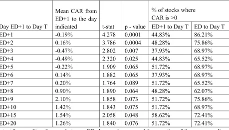
The effective day or the actual day of inclusion abnormal stock returns are expected to significantly positive due to the action of index funds. Hence only the stocks with positive ED abnormal returns are considered for testing the price pressure hypothesis in the Indian stock market. This is more appropriate because price pressure hypothesis postulates complete reversion of positive ED abnormal returns once the temporary excess demand of the index funds is satisfied. . The ED abnormal return for the stocks added to Nifty index for the period 1999-2010, with positive abnormal return on ED, is 3.18%. The results are displayed in Table 5.
Table 5. Mean Cumulative Abnormal Return from ED+1 to Day T for the 29 stocks added to Nifty index between 1999-2010 and for which ED abnormal return is greater than zero.
Day ED+1 to Day T
Mean CAR from ED+1 to the day
indicated t-stat p - value
% of stocks where CAR is >0
ED+1 to Day T ED to Day T
ED+1 -0.19% 4.278 0.0001 44.83% 86.21%
ED+2 0.16% 3.786 0.0004 48.28% 75.86%
ED+3 -0.47% 2.802 0.007 37.93% 68.97%
ED+4 -0.49% 2.320 0.025 44.83% 65.52%
ED+5 -0.22% 1.909 0.065 51.72% 68.97%
ED+6 0.14% 1.882 0.065 37.93% 68.97%
ED+7 0.20% 1.764 0.089 51.72% 65.52%
ED+8 0.90% 1.890 0.064 48.28% 62.07%
ED+9 2.10% 1.858 0.073 51.72% 75.86%
ED+10 1.42% 1.843 0.075 51.72% 68.97%
ED+15 1.54% 2.058 0.048 58.62% 72.41%
ED+20 1.26% 1.840 0.076 51.72% 72.41%
t-test for equality of means between ED abnormal return and the negative of the corresponding day ED+1 to day ‘T’ CAR. Satherthwaite's approximation for degrees of freedom is used. N= 29, includes only the stocks which had positive ED abnormal return. Two tailed t -test of whether the negative of the mean of the cumulative is equal to the mean of ED abnormal return using cross-sectional data.
The results of the t-test show that CAR from ED+1 through to ED+20 reject the null hypothesis that the mean of the ED abnormal return is equal to the negative of the CARs from ED+1 to ED+20 (at least the 10% level of significance). The maximum reversion is only -0.49% and takes place on ED+4. The results provide little evidence of price reversal and hence do not support the price pressure hypothesis in the Nifty index additions. Even in the complete sample(N=38), the maximum reversion of 1.1% and 0.89% occurs at ED+3, ED+4(release ending day) respectively compared to ED abnormal return of 1.92%. Therefore it seems reasonable to conclude that evidence in support of price pressure is limited at best. The result for price pressure is not consistent with some of the results from developed markets who have evidenced significant reversals following ED abnormal return.
4.5 Long term effect Window– ED+30 to ED+60
Table 6 Long term window12
Variable Mean Control Mean
% of stocks where variable >1 for ratios
and >0 for CAR Median
CAR 3.07% NA 53% 2.10%
t-stat 1.420* NA
Volume Ratio 1.71 1.14 44% 0.925
t-stat 2.006** 1.001
Liquidity Ratio 1.59 1.24 58% 1.11
t-stat 2.485*** 1.935**
Long term window represents ED+30 to ED+60 for the stocks added to Nifty index between 1999-2010. Complete sample,N=38. Control mean is calculated after removing the top 3 outliers on the higher side whenever both the % of stocks where VR >1 or CAR>0 is less than 50% and the median values suggest that few stocks influence the mean. One-tailed t-test to test whether the mean is greater than '0' or the ratios are greater than '1'.
***, **, * denotes significance at 1%,5%,10% level.
Table 6 reports the results for the long term window. CAR, volume ratio and liquidity ratio are significant at 10%, 5% and 1% level respectively. But the median value being less than one and the percentage of stocks with VR>1 being only 44% suggests that few outliers are influencing the result as far as the VR is concerned. As explained in section 4.3, a control mean was calculated for VR which was not significant even at 10% level. It is seen that for stocks included in the index the long run window CAR is statistically and economically significant. The increase in liquidity is even more significant because the buy and hold action of index funds around ED should theoretically reduce liquidity. Though liquidity is one of the Nifty addition criteria, this study compares post addition liquidity is compared with liquidity just before announcement. This makes the significant increase in liquidity in the long run window all the more interesting.
According to Chen et al (2004), liquidity can improve without information production if there is a corresponding increase in volume. In this case, though there is clear evidence towards liquidity improvement subsequent to inclusion, corresponding increase in volume is not supported. This result supports the information assertion around index announcements in the Nifty additions. The long term improvement in liquidity for added firms is similar to Chen et al(2004) in the US stock market. Li and Sadeghi(2009) and Hacibedel(2008) analysing the emerging markets evidence significant long term improvement in liquidity.
12 For the ‘long term window’, instead of Kotak Bank, data of Reliance capital was used. The Reliance capital
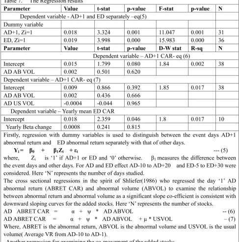
4.6 The Regression results
The earlier results in this study have evidenced the presence of significant ‘AD effect’ and ‘ED effect’. Now a hitherto not resorted to technique using ‘Dummy’ variables in eq (5) is used to confirm the earlier results. The period AD-10 to AD+20 and ED-5 to ED+30 is considered for the AD effect and ED effect respectively. The results in Table 7 show significant slope coefficients for both the effects. The intercept(not shown) representing the mean value of abnormal returns excluding AD+1(ED) for the considered period was marginally negative and not significant at any level. The results were consistent with the earlier results for both the sub periods.
According to Shiefler (1986), a significant positive slope in the cross sectional regression between abnormal AD return13 and abnormal AD volume is consistent with DSDC hypothesis. Further, Shiefler (1986) states that due to standard errors, the slope co-efficient may be biased towards zero and hence suggest introducing ‘usual volume’ (before AD volume) independently in the earlier regression. A significantly positive abnormal volume slope co-efficient and significantly negative usual volume slope co-efficient are consistent with DSDC hypothesis.
The regression results are tabulated in the table 7. The results for eq (6) show that even though the slope co-efficient is of proper sign, it is not significant at any reasonable level of significance. Similarly the results for eq (7) show that though the sign of the co-efficients are of the expected sign, both the slope co-efficient are not statistically significant even at 10% level. The Durbin Watson statistic (DW stat) is closer to two which suggests that the regression error terms are not correlated which is one of the assumptions14 of the regression. Further, according to Lynch and Mendenhall (1997), a significantly positive mean CAR over the run up window(AD+3 to ED-1) is supportive of the DSDC hypothesis. Table 3 shows that the run-up window CAR for the complete period is 0.2%, which is also not significant at any level of significance.
13 The AD window CAR was regressed with three day AD window abnormal volume which evidenced similar results. However, in deference to researchers who have evidenced that ‘averaging’ leads to spurious autocorrelation, the same was not shown. Our stand was vindicated when the DW stat improved from an acceptable 1.5 to a significant 1.84.
Table 7. The Regression results
Parameter Value t-stat p-value F-stat p-value N
Dependent variable - AD+1 and ED separately –eq(5)
Dummy variable
AD+1, Zi=1 0.018 3.324 0.001 11.047 0.001 31
ED, Zi=1 0.019 3.998 0.000 15.983 0.000 36
Parameter Value t-stat p-value D-W stat R-sq N
Dependent variable – AD+1 CAR- eq (6)
Intercept 0.015 1.799 0.080 1.84 0.002 38
AD AB VOL 0.002 0.501 0.620
Dependent variable – AD+1 CAR- eq (7)
Intercept 0.009 0.866 0.392 1.85 0.017 38
AD AB VOL 0.002 0.436 0.666
AD US VOL -0.0004 -0.044 0.965
Dependent variable – Yearly mean ED CAR
Intercept 0.018 2.359 0.046 1.8 0.017 10
Yearly Beta change 0.0008 0.241 0.815
Firstly, regression with dummy variables is used to distinguish between the event days AD+1 abnormal return and ED abnormal return separately with that of other days.
Yi = β0 + β1Zi + εi --- (5)
where, Zi is ‘1’ if AD+1 or ED and ‘0’ otherwise. β1 measures the difference between
the event days and other days. For AD and ED effect AD-10 to AD+20 and ED-5 to ED+30 were considered. Here ‘N’ represents the number of days studied.
The cross sectional regressions in the spirit of Shliefer(1986) who regressed the day ‘1’ AD abnormal return (ABRET CAR) and abnormal volume (ABVOL) to examine the relationship between abnormal return and abnormal volume as a significant slope co-efficient is consistent with downward sloping curves for the added stocks. Here ‘N’ represents the number of stocks. AD ABRET CAR = α + ψ * AD ABVOL -- (6) AD ABRET CAR = α + ψ * AD ABVOL + µ * USVOL – (7) Where, ABRET is the abnormal return, ABVOL is the abnormal volume and USVOL is the usual volume( Average VR from AD-10 to AD-1).
Another regression for examining the co-movement of the added stocks
Rit = α + β * Rmt + εit -- (8)
Where, Rit is stock return, Rmt is the Nifty index return on day ‘t’ and εit is a random variable with
expected value of zero and assumed to be uncorrelated. The daily pre-event regression is run for the period AD-70 to AD-10. The daily post event regression is run for ED+10 to ED+70. The difference βc calculated for each added stock by subtracting the pre- event beta from the post event beta is regressed with yearly ED CAR. Here ‘N’ represents number of years used in the regression. ***. **. * denote significance at 1%, 5%, 10% level respectively.
window CAR, evidences a negative CAR of -2.39%. The above results in Table 7 and the result that nifty inclusion is characterized by permanent abnormal return without corresponding permanent abnormal volume do not support DSDC hypothesis as the major explanation for the abnormal permanent return around index announcement in the Indian stock market.
4.7 Co-Movement
The beta change βc is calculated as the difference between the slope parameters of pre
addition and post addition regressions (eq (8)). The hypothesis that βc is greater than zero is
first tested using one-tailed t-test. The mean beta change βc is a statistically significant 0.14
and the number of stocks with positive beta change is 58%. Barberis et al (2005) have suggested that the non-informational view of stock inclusion is supported, if the effect(βc)is
stronger in the latest data along with the growth of index funds15. The data in Appendix 2 shows that βc is not stronger in the latest data.
Further, in order to verify the information effect, the yearly average beta change from 1999 -2010 is regressed with the yearly average value under mutual funds in India. Table 7 shows the slope co-efficient of the regression to be 0.0008 and is not statistically significant at any level of significance. The result evidencing lack of correlation between the mutual fund growth and beta change which should have been the case if the significant positive beta change is due to portfolio rebalancing actions of the mutual funds (index funds) supports the information-view in the Indian stock market.
The permanent index addition effect, for at least 80 days , may be due to positive information the index addition conveys regarding added stocks. It appears that the informed investors cause the initial price increase around AD and the index funds around ED. The uninformed investors then start investing in the added stocks. The other reason may be that the added stocks give positive signal to the investors in general and foreign institutional investors in particular regarding the quality of the stocks. Even the ‘habitat’ view, which according to Barberis et al(2005) studying S&P 500 supports the no-information view, may not apply to emerging markets. The reasons may be that, unlike the developed markets, emerging markets like the Indian stock market suffer from both lack of information efficiency and cost of information and hence are characterised by quality gaps between various groups of assets. These dissimilarities between the developed markets and the emerging market like India may be driving the evidenced results following Nifty index additions. The results are consistent with the findings of other emerging market studies of Li and Sadeghi(2009) and Hacibedel(2008). The results are also consistent with Chen et al(2004).
The observed results are interesting vis-a-vis the efficient market hypothesis(EMH) according to which any information is reflected instantaneously in the stock prices. According to the widely accepted martingale model of the efficient market hypothesis, a market is efficient with respect to any information if no economic profits accrue based on the information. Li and
Sadeghi(2009) state that under EMH there should be no price or liquidity effects. This study argues that index additions being information, there will be price and liquidity effects. Consequently, only the slow adjustment to market information is not consistent with EMH. The results in this study suggest slow adjustment16 to index addition information and economic profits which is not consistent with the efficient market hypothesis and constitutes a significant anomaly.
5. Conclusion
This study set out to analyse the price and volume effect surrounding Nifty index additions over the period 1999-2010. This study focused on two issues, the permanent effect and the information content of index additions. This study evidences that Nifty index additions are characterized by permanent abnormal returns subsequent to announcement and inclusion similar to the effects seen in the developed markets. But the evidence for permanent abnormal volume is limited unlike the developed markets.
Nifty index additions appear to convey information. Neither the DSDC hypothesis nor the price pressure hypotheses appears to be the major explanation for the observed permanent abnormal return around Nifty index additions. Further the permanent abnormal returns and increased liquidity subsequent to index additions is not accompanied by abnormal volume. Finally, the significant beta increase subsequent to addition is not the strongest in the latest data and there is no correlation between mutual fund growth and beta change. The evidence for the more recent sub-period sample is particularly important as it reflects the current market environment. The results for the second period (2007-2010) evidence increased price and information effect around index announcement and subsequent to inclusion. The results are consistent with other studies on emerging markets.
The increasing participation of foreign investors in the Indian stock market may be one of the reasons for the Nifty additions to convey information. Due to information asymmetry, investors in general and foreign investors in particular might perceive Nifty index inclusion as a signaling event regarding the quality of a stock. This appears to produce significant abnormal return directly without much abnormal volume. As the Indian stock market is characterized by constantly increasing foreign investments, the stronger ‘AD effect’ in the later period also supports the preceding assertion. Further, the cost of information in the markets like India affects the required rate of return and consequently the stock prices. Inclusion to benchmark index like Nifty might increase the visibility of the stocks for investors and reduce the cost of information. This brings into focus ‘investor awareness hypotheses’. Finally, the slow adjustment to Nifty index addition information is not consistent with market efficiency in the Indian stock market.
This study has bought issues which require further research. One such issue may be to delineate between the various ‘information supportive’ explanations in the Indian stock market. Another issue may be further research into the various co-movement hypotheses in the Indian stock market.
Acknowledgement:
I thank Dr. Victor Louis Anthuvan, Professor of Finance, Chairperson PhD, Loyola Institute of Business Administration, Chennai-600034, for his guidance and support throughout the study. I also thank the anonymous referees for their constructive suggestions.
References
Amihud, Y., Mendelson, H. (1986). Asset pricing and the bid-ask spread. Journal of Financial Economics, 17, 223-249.
Barberis, N., Shliefer, A., Wurgler, J. (2002). Comovement. NBER working paper No.8884.
Barberis, N., Shliefer, A., Wurgler, J. (2005). Comovement. Journal of Financial Economics,
75, 283-317.
Bekaert, G., Harvey, C.R. (2003). Emerging market finance. Journal of Empirical Finance, 10,
3-55.
Beneish, M.D., Whaley, R.E. (1996). The anatomy of the S&P game: The effect of changing rules. Journal of Finance, 51, 1909-1930.
Brennan, M.J., Chordia, T., Subrahmanyam, A. (1998). Alternative factor specifications, security characterstics, and the cross section of expected returns. Journal of Financial Economics, 49, 345-372.
Brown, S.J., Warner, J.B. (1985). Using daily stock returns: The case of event studies. Journal of Financial Economics, 14(1), 3-31.
Chakrabarti, R., Huang, W., Jayaraman, N., Lee, J. (2005). Price and volume effects of changes in the MSCI indices – nature and causes. Journal of Banking and Finance, 29,
1237-1264.
Chen, H., Noronha, G., Singhal, V. (2004). The price response to S&P 500 additions and deletions: Evidence of asymmetry and a new explanation. Journal of Finance, 59(4),
1901-1929.
Denis, D.K., McConnell, J.J., Ovtchinnikov, A.V., Yu, Y. (2003). S&P 500 Index additions and earnings expectations. Journal of Finance, 58, 1821-1840.
Dhillon, U., Johnson, H. (1991). Changes in the Standard and Poor’s 500 list. Journal of Business, 64, 75-85.
Elliot. W., Warr. R. (2003). Price pressure on the NYSE and the Nasdaq: Evidence from the S&P 500 index changes. Financial Management, Autumn 85-99.
effect?, An analytical survey, Financial Management, 35, 31-48.
Fama, E.F., (1970). Efficient Capital Markets: a Review of Theory and Empirical Work.
Journal of Finance, 25(1), 383–417.
Fama, E.F., (1991). Efficient Capital Markets: II. Journal of Finance, 46(5), 1575–1617.
Harris, L., Gurel, E. (1986). Price and volume effects associated with changes in the S&P 500 list, New evidence for the existence of price pressures. Journal of Finance, 41, 815-829.
Hacibedel, B., (2008). Index changes in emerging markets. Swedish Institute of financial research working paper, saltmatagatan, 19A, SE-113, 59, Stockholm, Sweden.
Hrazdil, K., (2009) The price, liquidity and information asymmetry changes associated with new S&P 500 additions. Managerial Finance, Vol. 35 Iss: 7, pp.579 – 605.
Jain, P.C., (1987). The effect on stock price of inclusion in or exclusion from the S&P 500.
Financial Analyst Journal, 43, 58-65.
Kumar, S.S.S., (2005). Price and volume effects of S&P Nifty index reorganizations. NSE
Research Initiative, working paper no. 90,
http://www.nseindia.com/content/research/comppaper90.pdf.
Li. Y., Sadeghi. M. (2009). Price performance and the liquidity effects of Index additions and deletions – Evidence from Chinese equity market. Asian Journal of Finance and Accounting,
Vol I, No 2:E2.
Lynch, A., Mendenhall, R. (1997). New evidence on stock price effects associated with changes in the S&P 500. Journal of Business, 70, 351-384.
Mackinlay, A.C., (1997). Event studies in economics and finance. Journal of Economic Literature, 35(1), 13-39.
Mase, B., (2002). The impact of changes in the FTSE 100 index. Brunel Department of Economics and Finance, Discussion paper, 02-25.
Merton, R.C., (1987). A simple model of capital market equilibrium with incomplete information. Journal of Finance, 42, 483-510.
Shleifer, A., (1986). Do demand curve for stocks slope down?. Journal of Finance, 41,
579-590.
Vijh, A.M., (1994). S&P 500 trading strategies and stock betas. Review of Financial Studies,
7, 215-251.
Wurgler, J., Zhuravskaya, E.(2002). Does arbitrage flatten demand curve for stocks?. Journal of Business, 75, 583-608.
Appendix
AD STOCK SYMBOL ED
24-Feb-10 KOTAKBANK 08-Apr-10
04-Sep-09 JP ASSOCIAT 22-Oct-09
04-Sep-09 IDFC 22-Oct-09
19-May-09 JINDALSTEEL 17-Jun-09
10-Feb-09 AXISBANK 27-Mar-09
29-Jul-08 RELIANCE POWER 10-Sep-08
31-Jan-08 DLF 14-Mar-08
26-Feb-08 POWERGRID 14-Mar-08
30-Oct-07 IDEA 12-Dec-07
30-Oct-07 CAIRN 12-Dec-07
11-Sep-07 UNITECH 05-Oct-07
10-Aug-07 NTPC 24-Sep-07
20-Feb-07 RPL 04-Apr-07
20-Feb-07 STERLITE 04-Apr-07
12-May-06 SUZLON 27-Jun-06
12-May-06 SIEMENS 27-Jun-06
12-Jan-05 TCS 25-Feb-05
26-Mar-04 ONGC 12-Apr-04
16-Jan-04 BHARTI 01-Mar-04
16-Jan-04 MARUTI 01-Mar-04
16-Jun-03 SAIL 04-Aug-03
13-Mar-03 GAIL 2-May-03
13-Mar-03 NATIONAL ALUMUNIUM 2-May-03
16-Sep-02 BPCL 28-Oct-02
16-Sep-02 HCLTECH 28-Oct-02
16-Sep-02 SCI 10-Oct-02
15-Apr-02 VSNL 31-May-02
14-Dec-01 SUNPHARMA 17-Jan-02
14-Dec-01 WIPRO 17-Jan-02
20-Jul-00 DIGITAL EQUIPMENTS 01-Sep-00
24-Apr-00 HCL-INSYS 24-May-00
24-Apr-00 ZEETELE 24-May-00
26-Apr-00 DABUR 10-May-00
03-Aug-99 BRITANNIA 08-Sep-99
03-Aug-99 SATYAM COMPUTERS 08-Sep-99
19-Apr-99 DRREDDY 26-May-99
19-Apr-99 NOVARTIS 26-May-99
Appendix 2.Yearwise ED abnormal return and Beta change is given for the period 1999-2010 in order to verify whether the beta change is stronger in the latest data
Year
ED Abnormal return
Number of
additions BETA Change
Average assets under Mutual funds in Rs. Crores
1999 3.60% 5 -0.182 97028 2000 2.20% 4 0.249 99326
2001 NA - 0.249 101822
2002 0.60% 6 0.227 122660 2003 -0.82% 3 -0.183 140093 2004 2.28% 3 -0.098 150537 2005 3.29% 1 0.516 199248 2006 0.51% 2 0.263 323597 2007 4.89% 6 0.237 549936 2008 3.68% 3 -0.184 421117 2009 -0.50% 5 -0.011 794486
The average assets under mutual fund as on december-31 of each year
Appendix 4. Pictorial representation of VR around AD and ED as in Table 4
Copyright Disclaimer
Copyright reserved by the author(s).