Futures Trading and Its Impact on Volatility of Indian
Stock Market
Namita Rajput
E-mail: namitarajput27@gmail.com
Ruhi Kakkar
E-mail: ruhi.kakkar@gmail.com
Geetanjali Batra
E-mail: ms.geetanjali.batra@gmail.com
Received: July 29, 2012 Accepted: December 14, 2012 Published: June 1, 2013
doi:10.5296/ajfa.v5i1.2165 URL: http://dx.doi.org/10.5296/ajfa.v5i1.2165
Abstract
Derivative products like futures and options are important instruments of price discovery, portfolio diversification and risk hedging. This paper studies the impact of introduction of index futures on spot market volatility on S&P CNX Nifty using Bi-Variate E-GARCH technique. The evidence of this model shows that the volatility spillover between spot and futures markets is uni-directional from spot to futures and spot market dominates the futures market in terms of return and volatility. The volatility persistence and clustering is found to be significant and bidirectional at 5 % level of significance. At the practical level, a better understanding of the mean and variance dynamics of the spot and futures market can improve risk management and investment decisions of the market agents. The findings have implications for policy makers, hedgers and investors. The research contributes to literature for emerging markets such as India.
Keywords: Derivatives, index futures, stock markets, volatility, ARCH-GARCH, Spillover
Introduction
The liberalization and integration of financial markets globally has created new investment opportunities, which in turn require the development of new instruments that are more proficient to deal with the increased risks. Investors who are actively engaged in industrial and emerging markets need to hedge their risks from these internal as well as cross-border transactions. Agents in liberalized market economies who are exposed to volatile stock prices and interest rate changes entail suitable hedging products to pact with them. With the advent of liberalisation and economic expansion in these emerging economies demands that corporations should discover better ways to manage financial and commodity risks. The most wanted instruments that allow market participants to manage risk in the modern securities trading are known as derivatives which are a new advent in developing countries compared to developed countries. The main reason behind the derivatives trading is that derivatives reduce the risk by providing an additional way to invest with lesser trading cost and it facilitates the investors to extend their settlement through the future contracts. It provides extra liquidity in the stock market. They represent contracts whose payoff at expiration is determined by the price of the underlying asset—a currency, an interest rate, a commodity, or a stock. Derivatives are traded in organized stock exchanges or over the counter by derivatives dealers. The impact of derivatives trading on stock market volatility has received considerable attention in India, particularly after the stock market crash of 2001. Derivative products like futures and options have become important instruments of price discovery, portfolio diversification and risk hedging. In the last decade, many rising and transition economies have started introducing derivative contracts. Derivatives markets have been in existence by many accounts even longer than that for securities. However, it has been their growth in the past 30 years that has made them a significant segment of the financial markets.
price stabilization, encouraging competition, increasing efficiency, inherent leverage, low transaction costs, and lack of short sale restrictions as well as fulfilling desires of speculators are some of the prime economic functions of the futures market.
Price discovery and risk transfer are considered to be two major contributions of futures market towards the organization of economic activity (Garbade and Silber, 1983). Price discovery refers to the use of future prices for pricing cash market transactions. This implies that futures price serves as market’s expectations of subsequent spot price. Understanding the influence of one market on the other and the role of each market segment in price discovery is the central question in market microstructure design and is very important to academia and regulators.
Price of the derivative is derived from the underlying asset, any change in price of the underlying asset leads to change in the value of the asset. Derivatives facilitate investment and arbitrage strategies that straddle market segments. It helps to increase asset substitutability, both domestically and internationally. Derivatives help to improve liquidity. It helps to facilitate the creation of pay off characteristics at a lower cost that would result from the acquisition of underlying assets. Derivative markets help increase savings and investment in the long run.
The derivative market performs a number of economic functions. Some of them are given below:
The prices of derivatives converge with the prices of the underlying at the expiration of derivative contract. Thus derivatives help in discovery of future as well as current prices.
An important subsidiary benefit that flows from derivatives trading is that it acts as a catalyst for new entrepreneurial activity.
Derivatives markets help boost savings and investment in the long run. Transfer of risk enables market participants to expand their volume of activity.
market in order to cover the risk exposure that they challenge. Considerable amount of research work has been conducted in the field of volatility and its spillover, the results of which are mixed. For modeling volatility the work done by Pre-eminence of Bollerslev (1986), Engle (1982), Bollerslev and Engle (1986) is noteworthy. Therefore, it has become necessary, from time to time, to conduct empirical studies to measure the impact of financial derivatives, on volatility spillover to spot market and vice-versa. Generally, volatility is considered as a measurement of risk in the stock market return and a lot of discussions have taken place about the nature of stock return volatility. Therefore, understanding factors that affect stock return volatility is an imperative task in many ways. Issues like price discovery and volatility spillover have been extensively researched for mature markets. The work is very limited for emerging markets in general and India in particular. In this backdrop, an attempt has been made to revisit the debate on volatility spillover in Indian stock market. It covers fairly longer study period compared to prior research of the subject. The study attempts to address the following questions:
Is there a volatility spillover from futures market to spot market and vice-versa?
The remainder of the paper is organized as follows. Section one gives review of literature and the relevance of study. Section two contains description of data and the methodology employed along with the empirical tests carried out. Section III exhibits analysis and interpretation of the data through a variety of tables into which relevant details have been compressed and summarized under appropriate heads and presented in the tables. Section IV provides brief summary, conclusion of the main findings, policy implications.
Review of Literature
Cox (1976) opine that the introduction of futures markets led to increase in informational efficiency, as futures are relatively inexpensive, have low margin requirements and low transaction costs. Figlewski (1978) suggests that the new traders in the GNMA market add noise to GNMA securities trading because of the introduction of futures trading. Cox, 1976; Stein, 1987; Ross, 1989, Chan et al.,1991 conclude that Index futures enable investors to trade large volumes at lower transaction costs, improve risk sharing and reduce volatility.
impact of S&P 500 index futures and options trading on the volatility of the firms' shares that comprise the S&P 500. He reports no significant difference in the volatility of the S&P 500 stocks as compared to a control sample of 500 matching shares in the period 1975 to1983 before the start of trade in index options and futures. However, after 1983, he reported statistically significant increase in the volatilities of firms in the S&P 500 index. He suggests that the change in volatility is not significant "economically" and that other factors could be responsible for the increase. Becketti and Roberts (1990) opine that futures contract is an agreement to exchange in future. It does not necessarily involve an exchange of assets in the future; the buyers and sellers of the index settle their positions by taking offsetting positions. Close to cessation, futures traders may close their positions by taking a position opposite to the initial one, by physical delivery, or by paying the difference between the futures price and the spot price of the underlying asset.
Hodgson et al., (1991) study the impact of All Ordinaries Share Index (AOI) futures on the Associated Australian Stock Exchanges over the All Ordinaries Share Index. They analyse data for a period of six years from 1981 to 1987. Standard deviation of daily and weekly returns is estimated to measure the change in volatilities of the underlying Index. The results indicate that the introduction of futures and options trading has not affected the long-term volatility, which reinforces the findings of the previous U.S. studies. Froot and Perold (1991) develop a model to demonstrate that futures markets cause an increase in the market depth due to the presence of more market makers in the futures segment than in the cash market and the more rapid dissemination of information.
Abhyankar (1995) concludes that lower transaction cost is the main reason for traders who have market wide information to use the futures market. Pericli and Koutmos (1997) analyse the impact of the US S&P 500 index futures on spot market volatility. Their results show that index futures do not increase spot market volatility. Dennis and Sim (1999) examine share price volatility with the introduction of individual share futures on the Sydney Futures Exchange by employing GARCH model. They conclude that the impact of futures trading on cash market volatility is not significant as compared to the impact of cash market trading. Gulen and Mayhew (2000) examine stock market volatility before and after the introduction of index futures in 25 countries. They find that index futures had no significant effect on the spot markets in all the countries excluding US and Japan. They also find that spot volatility was independent of changes in futures trading in 18 countries, and that spot volatility is negatively influenced by uninformed futures volume in Austria and the UK. Bologna and Cavallo (2002) examine the effect of the introduction of stock index futures on the volatility of the Italian spot market, and find a reduction in spot market volatility and enhanced market efficiency. They conclude that increased impact of recent news and a reduced effect of the uncertainty originating from the old news were the main reasons for this phenomenon.
are non-institutional investors who are generally un-informed and are prone to over react to the bad news. The introduction of the TAIEX futures trading improves the efficiency of information transmission from futures to spot markets. Raju and Karande (2003) find a reduction in spot market volatility after the introduction of index futures. Golaka C Nath (2003) investigates behaviour of stock Market volatility after introduction of derivatives by employing GARCH model. Using a sample of 20 stocks taken randomly from the NIFTY, he observes that for most of the stocks, the volatility comes down in the post derivative period while for only few stocks in the sample the volatility in the post derivatives remains same or increases marginally. Thenmozhi and Thomas (2004) conclude that there is a reduction in volatility in the underlying stock market and increased market efficiency following the launch of NIFTY-linked futures. Pok and Poshakwale (2004) study the impact of the futures trading on spot market volatility. They used data from both the underlying and non-underlying stocks of Malaysian stock market. They used GARCH to test time varying volatility and volatility clustering in data. They conclude that the initiation of futures trading increases spot market volatility and the flow of information to the spot market. The underlying stocks respond more to recent news whereas the non-underlying stocks respond to old news. Antoniou et al. (2005) examined the relationship between index futures and their underlying markets. Vipul (2006) investigate the effect of futures trading on volatility in Nifty and in individual stocks using data for the period from 1998 to 2004. Using GARCH model to capture volatility clustering phenomena in the data, he concludes that introduction of derivatives trading does not destabilize the stock market.
Schwert (1990), Backetti and Roberts (1990), Darrat and Rahman (1995), Kamara et al. (1992), Perieli and Koutmos (1997), Spyrou (2005), and Alexakis (2007) also confirmed the stabilisation theory. Suhasini Subramanian (2012), analyse contrasting theoretical approaches and empirical evidence relating to the impact of index futures on volatility and noise trading.
Data Base and Methodology
Index futures on S&P CNX Nifty were permitted for trading on National Stock Exchange (NSE) on 12th June, 2000. For the purpose of the current study on price discovery, Index futures on S&P CNX Nifty. Daily closing values of Index futures and S&P CNX Nifty have been taken from June, 2000 till March 2012. Returns ( Rt) have been calculated as log of ratio of present day’s price to previous day’s price (i.e. Rt = ln (Pt /Pt-1)). Data relating to the price series have been obtained from website of NSE (www.nseindia.com). Given the nature of the problem and the quantum of data, we first study the data properties from an econometric perspective and find unit root of the two series futures and spot. Further, to quantify and study volatility spillover, we use Bivariate EGARCH framework which is covered in the next section.
(1988) test of stationarity has also been performed for the series.
The error correction model takes into account the lag terms in the technical equation that invites the short run adjustment towards the long run. This is the advantage of the error correction model in evaluating price discovery. The presence of error correction dynamics in a particular system confirms the price discovery process that enables the market to converge towards equilibrium. In addition, the model shows not only the degree of disequilibrium from one period that is corrected in the next, but also the relative magnitude of adjustment that occurs in both markets in achieving equilibrium. Moreover, cointegration analysis delivers the message saying how two markets (such as futures and spot commodity markets) reveal pricing information that are identified through the price difference between the respective markets. The implication of cointegration is that the commodities in two separate markets respond disproportionately to the pricing information in the short run, but they converge to equilibrium in the long run under the condition that both markets are innovative and efficient. In other words, the root cause of disproportionate response to the market information is that a particular market is not dynamic in terms of accessing the new flow of information and adopting better technology. Therefore, there is a consensus that price change in one market (futures or spot commodity market) generates price change in the other market (spot or commodity futures) with a view to bring a long run equilibrium relation is :
Ft St t (1)
Equation (1) can be expressed as in the residual form as: ệ
FtSt ệ t (2)
In the above equations Ft and St are futures and spot prices of a commodity in the respective market at time t. Both α and β are intercept and coefficient terms, where as ệt is estimated white noise disturbance term. The main advantage of cointegration is that each series can be represented by an error correction model which includes last period’s equilibrium error with adding intercept term as well as lagged values of first difference of each variable. Therefore, casual relationship can be gauged by examining the statistical significance and relative magnitude of the error correction coefficient and coefficient on lagged variable. Hence, the error correction model is:
Ft f fet fFt1YfSt1ft
^
1 (3)
St s set^1 fSt1 YfFt1 St (4)
In the above two equations, the first part
e
t1 ^represents the short run effect of previous period’s change in price on current period’s deviation. The coefficients of the equilibrium error, αf and αs signify the speed of adjustment coefficients in future and spot commodity markets that claim significant implication in an error correction model. At least one coefficient must be non zero for the model to be an error correction model (ECM). The coefficient acts as an evidence of direction of casual relation and reveals the speed at which discrepancy from equilibrium is corrected or minimized. If, αf is statistically insignificant, the current period’s change in future prices does not respond to last period’s deviation from long run equilibrium. If both, αf and βf are statistically insignificant; the spot price does not Granger cause futures price. The justification of estimating ECM is to know which sample markets play a crucial role in price discovery process. Error Correction Terms (ECTS) also known as mean- reverting price process, provide some insights into the adjustment process of spot and future prices towards long run equilibrium. This implies that once the price relationship of spot and futures market deviates away from the long-run coinetgrated equilibrium, both markets will make adjustments to re-establish the equilibrium condition during the next period.
Bi-Variate EGarch Model and Volatility Spillover
In this section, we evaluate if there is any volatility spillover between future and spot market for the sample series. Volatility spillover reveals that future trading could intensify volatility in the underlying spot market due to the larger trading program and the speculative nature of the future trading. The volatility spillovers hypothesis involves testing for the lead-lag relations between volatilities in the futures and spot markets. Clearly, reliable tests require common good measure of volatilities. Bollerslev’s (1986) generalize autoregressive conditional heteroscedasticity (GARCH) model cannot be used due to certain regularities where it assumes that positive and error terms have a symmetric effect on the volatility. In other words, good news (market advances) and bad news (market retreats) have the same effect on the volatility in this model. This implies that the leverage effect (price rise and fall) is neutralized in this model. The second regularity is that all coefficients need to be positive to ensure that the conditional variance is never negative (i.e. measure of risk). To overcome these weaknesses of the GARCH model in handling financial time series, Nelson’s (1991) exponential GARCH (EGARCH) model is used in order to capture the asymmetric impacts of shocks or innovations on volatilities and to avoid imposing non-negativity restrictions on the values of GARCH parameters. There are many studies in which symmetries in stock return are documented [e.g., Nelson (1991), Koutmos and Booth (1995), Koutmos and Tucker (1996), Engle and Ng (1993), and Glosten et al. (1993)].
adjust to deviations from long-run price disequilibria, whereas traditional EGARCH models do not. As such, the model facilitates the testing of both short run and long run volatility spillovers hypotheses. The EC-EGARCH model may further prove useful for portfolio managers in formulating optimal hedging strategies. Some studies e.g., Yang, Bessler, and Leatham (2001) emphasize the need to incorporate any existing cointegration between spot and futures prices into hedging decisions, while others such as Lien and Lou (1994) underscore the importance of GARCH effects in such decisions.
We use the following EGarch Model
) ( ) ( ) ( )
ln( 2 1
1 2 1 2 2
ff t fs t f t
ft e f e s f
(5) ) ( ) ( ) ( )
ln( 2 1
1 2 1 2 2
ss t sf t f t
st e s e f s
(6)
The unrelated residuals eft and est are obtained from the equations (3) and (4). This two step approach (the first step for the VECM and the second step for the Bivariate EGARCH model is asymptotically equivalent to a joint estimation for the VECM and EGARCH models (Greene, 1997).
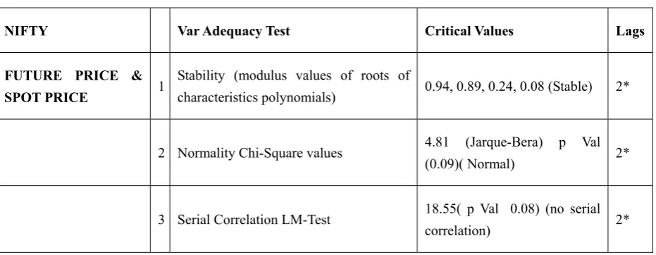
Before estimating the EGARCH model, it is necessary to check the model adequacy by performing the diagnostic tests that involve serial correlation, normally distributed error and goodness of fit measures. Hence we check the model adequacy test by testing Auto correlation LM Test, Normality Test and Var Stability Condition Test (AR Roots).
Analysis And Interpretation of Results
Table 1. Stationarity test for sample series
Price- Series Inference On Return Series Integration I (I)
ADF Test Phillips-Perron Test ADF Test Phillips-Perron Test
t-statistics t-statistics t-statistics t-statistics
NIFTY
(A)FUTURE PRICES -1.09 -0.51 -41.98 ** -41.98 **
(B) SPOT PRICES 1.12 -1.38 -41.35 ** -41.32 **
The table describes the sample price series that have been tested using Augmented Dickey Fuller (ADF) 1981. The ADF test uses the existence of a unit root as the null hypothesis. To double check the robustness of the results, Phillips and Perron (1988) test of stationarity has also been performed for the price series and then both the test are performed on return series also as shown in Panel-A (price series) and Panel B (Return series) are integrated to I(1). All tests are performed using 5%level of significance (**).
Before estimating the EGARCH model, it is necessary to check the model adequacy by performing the diagnostic tests that involve serial correlation, normally distributed error and goodness of fit measures. All diagnostic tests are primarily carried on the standardized residuals via OLS and it is found that all are significant at 5% level. The diagnostic statistics with respect to EGARCH model are reported in Table 2.
Table 2. Var adequacy test
NIFTY Var Adequacy Test Critical Values Lags
FUTURE PRICE &
SPOT PRICE 1
Stability (modulus values of roots of
characteristics polynomials) 0.94, 0.89, 0.24, 0.08 (Stable) 2*
2 Normality Chi-Square values 4.81 (Jarque-Bera) p Val (0.09)( Normal) 2*
3 Serial Correlation LM-Test 18.55( p Val 0.08) (no serial correlation) 2*
coefficient βsf indicates the volatility spillover from futures to spot and βfs means reverse direction. The coefficients βss and βff show the volatility clustering, while the coefficients λs and λf measure the degree of volatility persistence. The residuals of the model are tested for additional ARCH effects using ARCH LM test.
The results of volatility spillover from spot to future are significant as P-value of coefficient of βfs is < 0.05 at 5 % level of significance, it is not true in the reverse direction i.e. P-Value of βsf is > 0.05 i.e. no significant spillover is observed from future to spot see Table 3 panel (a) &Panel (b) respectively. This means innovations of spot markets have asymmetric influence to the variance of futures markets, and there is a uni-directional volatility spillover, from spot market to future market, or in simple words we can say that an innovation originating in spot market influences the volatility of the futures market.
Volatility persistence is tested for sample series to test the effect of shocks, which is an indicator of market efficiency. It means Persistence of volatility that today’s volatility is due to information that arrived today and will affect tomorrow’s volatility and volatility of days to come. γf and γs measure the persistence of volatility in spot and futures market. The smaller the absolute value of the coefficient, the less persistent volatility is after a shock. Volatility persistence is significant for both spot and future prices for sample series, as p (value) is coming less than 0.05 at 5 % level of significance with significant coefficients of λs and λf which is a measure the degree of volatility persistence.
Volatility estimation is important for several reasons and for different people in the market pricing of securities is supposed to be dependent on volatility of each asset. Market prices tend to exhibit periods of high and low volatility. This sort of behaviour is called volatility clustering. Volatility clustering is tested for sample series, which means “large changes tend to be followed by large changes, of either sign, and small changes tend to be followed by small changes.”
A quantitative manifestation of this fact is that, while returns themselves are uncorrelated, absolute returns |rt| or their squares display a positive, significant and slowly decaying autocorrelation function: corr (|rt|,|rt+τ |) > 0 for τ ranging from a few minutes to a several weeks. A significantly positive and asymmetrical influence of innovation is observed i.e. the market-specific volatility clustering coefficients are all positively significant at
5% level in the future and spot markets.
Table 3.Volatility relationship - dependent variable – future
Panel A: Coefficient std. error z-statistic prob.
a. βff (volatility clustering) sqrresidfuture(-1) -0.0 0.0 -2.01 0.0** b. βfs (volatility spillover) sqrresidspot(-1) 0.0 0.0 2.27 0.0** c. λf (volatility persistence) varfuture(-1) 0.94 0.0 210.71 0.0** Volatility Relationships - Dependent Variable –Spot
Panel B Coefficient std.
Error
z-statistic prob.
a. βss (volatility clustering) sqrresidspot(-1) 0.01 0.00 1.31 0.0** b. βsf (volatility spillover)
sqrresidfuture(-1) -0.0 0.01 -1.01 0.3
c. λs(volatility persistence) varspot(-1) 0.9 0.00 191.71 0.0**
The table describes volatility spillover (βsf and βfs) volatility persistence (λf and λs) and volatility clustering (βff
and βss) from the spot to future or future to spot respectively. Volatility spillover is observed from spot to future
and not vice versa. Volatility persistence is significant for both spot and future prices for all commodities and
indices, the market-specific volatility clustering coefficients βff and βss are all positively significant at 5% level in
the future and spot markets.
Conclusion
important vehicle of price discovery. For example, the information about instantaneous impact and lagged effects of shocks between spot and futures prices may be used in decision making regarding hedging activities (Wahab and Lashgari, 1993). A deep understanding of the dynamic relation of spot and futures prices and its relation to the basis provides these “agents” the ability to use hedging in a more skilled mode. Furthermore, if a return analysis is questionable, volatility spillovers provide an alternative measure of information transmission (Chan, Chan and Karolyi, 1991). Owing to these grounds, research committed to the relationship between futures and spot returns (first moments) has been capacious (Chan and Karolyi, 1991; Chan, 1992), with this interest growing to examining higher moment dependencies (time-varying spillovers) between markets (Ng and Pirrong, 1996; and Koutmos and Tucker, 1996).
The literature relating to volatility in stock futures market has mainly been confined to developed economies. Stock markets in emerging economies like India have been growing exponentially. Empirical Studies on the subject show that the introduction of derivatives contracts improves the liquidity and reduces informational asymmetries in the market. The present study evaluates volatility spillover effects for fairly large period in Indian stock market to bridge the important gap in the literature in a comprehensive way. We cover NIFTY indices and the study period is from June 2003-March 2012.We find that spot and futures a unidirectional volatility spillover is observed from spot to futures and not vice-versa. Whenever there is high volatility in stock market that will affect futures market. The findings of the study suggest that the Nifty spot are more important indicators of stock movements which is in contrary to the studies done by Kawaller, Koch and Koch (1987), Stoll and Whaley (1990) , Chan (1992) and Ghosh (1993) which reported dominant role of S&P 500 futures. In studies like Chan, Chan and Karolyi (1991), Arshanapali and Doukas (1994), Wang and Wang (2001), Mukherjee and Mishra (2004) bidirectional spillover (cross market spillover) is observed in both the markets.
References
Abhyankar, A. H. (1995). Return and Volatility Dynamics in the FTSE 100 stock index and
stock index futures market. Journal of Futures Market, 15(4), 457-488.
http://dx.doi.org/10.1002/fut.3990150405
Alexakis, P. (2007). On the Effect of Index Future Trading on Stock Market Volatility.
International Research Journal of Finance and Economics, 11, 7-20.
Antoniou, A., Koutmos, G., & Pericli, A. (2005). Index Futures and Positive Feedback Trading: Evidence from major stock exchanges. Journal of Empirical Finance, 12, 219–238. http://dx.doi.org/10.1016/j.jempfin.2003.11.003
Arshanapali, B., & Doukas, J (1994). Common Volatility in S&P 500 Stock Index S&P 500 Index Futures Prices during October 1987. Journal of Futures Markets, 14(8), 915- 925 http://dx.doi.org/10.1002/fut.3990140805
Becketti, S., & Roberts, D. -J. (1990). Will Increased Regulation of Stock Index Futures Reduce Stock Market Volatility? Economic Review, Federal Reserve Bank of Kansas City, 33–46.
Bollerslev, Tim. (1986). Generalized Autoregressive Conditional Heteroscedasticity. Journal of Econometrics, 31(3), 307-327. http://dx.doi.org/10.1016/0304-4076(86)90063-1
Bollerslev, T., Engle, R. F., & Nelson, D. (1994) ARCH Models, Handbook of Econometrics, 4, Chapter 49.
Bologna, P., & Cavallo, L. (2002). Does the Introduction of Stock Index Futures Effectively Reduce Stock Market Volatility? Is the ‘Futures Effect’ Immediate? Evidence from the Italian
Stock Exchange Using GARCH. Applied Financial Economics, 12, 183–92.
http://dx.doi.org/10.1080/09603100110088085
Chan, K., Chan, K. C., & Karolyi, A. G. (1991). Intraday Volatility in the Stock Index and Stock Index Futures Markets. The Review of Financial Studies, 4(4), 657–684. http://dx.doi.org/10.1093/rfs/4.4.657
Chan, K. (1992). A Further Analysis of the Lead-lag Relationship between the Cash Market and Stock Index Futures Market. Review of Financial Studies, 5(1), 123-152. http://dx.doi.org/10.1093/rfs/5.1.123
Chiang, H. C., & C. Y., Wang (2002), The Impact of Futures Trading on the Spot Index Volatility: Evidence for Taiwan Index Futures. Applied Financial Letters, 9, 381-385.
Cox, C. C. (1976). Futures Trading and Market Information. Journal of Political Economy, 84, 1215–1237. http://dx.doi.org/10.1086/260509
Darrat, A. F., & Rahman, S. (1995). Has Futures Trading Activity Caused Stock Price
Volatility? Journal of Futures Markets, 15, 537–557.
Dennis S. A., & A. B. Sim (1999), Share Price Volatility with the Introduction of Individual Share Futures on Sydney Futures Exchange. International Review of Financial Analysis, 8,
153-163. http://dx.doi.org/10.1016/S1057-5219(99)00013-7
Dickey, David A., & Fuller, Wayne A., (1981). Likelihood Ratio Statistics for Autoregressive Time Series with a Unit Root. Econometrica, Econometric Society, 49(4), 1057-72.
Edwards, R. F. (1988a). Does Futures Trading Increase Stock Market Volatility? Financial Analyst Journal, 44, 63–69. http://dx.doi.org/10.2469/faj.v44.n1.63
Edwards, R. F. (1988b). Policies to Curb Stock Market Volatility. Columbia University Working Papers, 141–184.
Engle, R.F. (1982). Autoregressive Conditional Heteroscedasticity with Estimates of The Variance of United Kingdom Inflation. Econometrica, 50(4), 987-1008. http://dx.doi.org/10.2307/1912773
Engle, R.F. & Ng, V. (1993). Measuring and Testing the Impact of News on Volatility. The Journal of Finance, 48, 1749-1778. http://dx.doi.org/10.2307/2329066
Figlewski, S. (1978). Market “Efficiency” in a market with Hetrogeneous Information.
Journal of Political Economy, 86(4), 581-597. http://dx.doi.org/10.1086/260700
Figlewski, S. (1981). Futures Trading and Volatility in the GNMA Market. Journal of Finance, 36(1), 445-56. http://dx.doi.org/10.2307/2327030
Froot, K. A., & Perold, A. F. (1995). New Trading Practices and Short-run Market Efficiency.
The Journal of Futures Markets, 15(7), 731-765. http://dx.doi.org/10.1002/fut.3990150702
Garbade K.D., & Silber W.L. (1983). Price Movements and Price Discovery in Futures and
Cash Markets. The Review of Econometrics and Statistics, 65(2),
289-297.http://dx.doi.org/10.2307/1924495
Greene, W. (1997). Econometric Analysis, 3rd Edition. MacMillan Publishing Company, New York.
Ghosh, A (1993). Cointegration and Error Correction Models: Intertemporal Causality between Index and Futures Prices. Journal of Futures Markets, 13(2), 193-198. http://dx.doi.org/10.1002/fut.3990130206
Gulen, H., & Mayhew, S. (2000). Stock Index Futures Trading and Volatility in International
Equity Markets. The Journal of Futures Market, 20(7), 661–685.
http://dx.doi.org/10.1002/1096-9934(200008)20:7<661::AID-FUT3>3.0.CO;2-R
Glosten, L. R., R. Jaganathan, & D. E. Runkle (1993), On the Relation between the Expected Value and the Volatility of the Nominal Excess Returns on Stocks. Journal of Finance, 48(4), 1779-1801. http://dx.doi.org/10.2307/2329067
Hodgson, A., & Nicholas, D. (1991). The Impact of Index Futures on Australian Share Market Volatility. Journal of Business and Accounting, 12(l), 645-658.
Kamara, A. (1992). The effect of futures trading on the stability of standard and poor 500
returns. Journal of Futures Markets, 12(6), 645–658.
http://dx.doi.org/10.1002/fut.3990120605
Kawaller, I. G., Koch, P. D., & Koch, T. W. (1987). The Temporal Price Relationship between S&P 500 Futures and the S&P Index. Journal of Finance, 42, 1309–1329. http://dx.doi.org/10.1111/j.1540-6261.1987.tb04368.x
Kavussanos M.G., & Visvikis, I.D. (2004). Market interactions in returns and volatilities between spot and forward shipping freight markets. Journal of Banking & Finance, 28(8), 2015–2049. http://dx.doi.org/10.1016/j.jbankfin.2003.07.004
Koutmos G. and Booth G.G. (1995). Asymmetric volatility transmission in international stock
markets. Journal of International Money and Finance, 14(6), 747–762.
http://dx.doi.org/10.1016/0261-5606(95)00031-3
Koutmos G., & Tucker M. (1996). Temporal relationships and dynamic interactions between
spot and futures stock markets. Journal of Futures Markets, 16(1), 55–69.
http://dx.doi.org/10.1002/(SICI)1096-9934(199602)16:1<55::AID-FUT3>3.0.CO;2-G
Lien, D., & Lou, X. (1994). Multiperiod Hedging in presence of conditional
Heteroscedasticity. Journal of Futures Markets, 14, 927-955.
http://dx.doi.org/10.1002/fut.3990140806
Mukherjee, K., & Mishra, R K. (2004). Lead-lag Relationship between Equities and Stock Index Futures Markets and its Variation around Information Release: Empirical Evidence from India. NSE website.
Ng, V K., & Pirrong, S C (1996). Price Dynamics in Refinery Petroleum Spot and Futures
Markets. Journal of Empirical Finance, 2(4), 359-388.
http://dx.doi.org/10.1016/0927-5398(95)00014-3
Nath, G. C. (2003). Behaviour of Stock Market Volatility after Derivatives. NSE Working Paper.
Perieli, A., & Koutmos, G. (1997). Index Futures and Options and Stock Market Volatility.
Journal of Futures Markets, 18(8), 957–974.
http://dx.doi.org/10.1002/(SICI)1096-9934(199712)17:8<957::AID-FUT6>3.0.CO;2-K
Philips. P., & Perron. P. (1988). Testing for a Unit Root in Time Series Regression.
Biometrica, 75, 335-46. http://dx.doi.org/10.1093/biomet/75.2.335
Raju, M. T., & Karande, K. (2003). Price Discovery and Volatility on NSE futures Market.
SEBI Bulletin, 1(3), 5–15.
Ross, S. A. (1989). Information and Volatility: The no-arbitrage martingale approach to
Timing and resolution irrelevancy. Journal of Finance, 44, 1–17.
http://dx.doi.org/10.2307/2328272
Schwert, G. W. (1990). Stock Volatility and the Crash of ’87. Review of Financial Studies, 3,
77–102. http://dx.doi.org/10.1093/rfs/3.1.77
Spyrou, S. I. (2005). Index Futures Trading and Spot Price Volatility: Evidence from an
Emerging Market. Journal of Emerging Market Finance, 4(2), 151–167.
http://dx.doi.org/10.1177/097265270500400203
Subramanian S. (2012). The Impact of the Introduction of Index Futures on Volatility and
Noise Trading. National Stock Exchange Limited. www.nseindia.com/research/content/RP_5_Mar2012.pdf
Stein, J. (1987). Informational Externalities and Welfare-Reducing Speculation. Journal of Political Economy, 95, 1123–1145. http://dx.doi.org/10.1086/261508
Stoll, H R., & Whaley, R E (1990). The Dynamics of Stock Index and Stock Index Futures
Returns. Journal of Financial and Quantitative Analysis, 25(4), 441-468.
http://dx.doi.org/10.2307/2331010
Thenmozhi, M. (2002). Futures Trading, Information and Spot Price Volatility of NSE-50 • Index Futures Contract. NSE Research Paper, National Stock Exchange of India Ltd.
Vipul. (2006). The Impact of the Introduction of the Derivatives on Underling Volatility: Evidence from India. Journal of Applied Financial Economics, 16(9), 687-694.
Wahab, M., & Lashgari, M. (1993). Price Dynamics and Error Correction in Stock Index and Stock Index Futures Markets: A Cointegration Approach. Journal of Futures Markets, 13(7), 711-742. http://dx.doi.org/10.1002/fut.3990130702
Wang, P., & Wang, P. (2001). Equilibrium Adjustment, Basis Risk and Risk Transmission in Spot and Forward Foreign Exchange Markets. Applied Financial Economics, 11(2), 127-136. http://dx.doi.org/10.1080/096031001750071514