Accounting for Tuition Increases across U.S. Colleges
∗Grey Gordon Indiana University†
Aaron Hedlund University of Missouri‡ March 19, 2018
Abstract
This paper uses detailed institution-level data and an equilibrium model to assess differ-ent theories for the steep, persistdiffer-ent rise in college tuition. The framework embeds quality-maximizing, imperfectly competitive colleges into an incomplete markets, life-cycle environment with student loan borrowing and default. We measure the contribution of supply-side factors— namely, Baumol’s cost disease and changes in the availability of non-tuition revenue sources—as well as demand-side forces, such as evolutions in labor market conditions and changes to the Federal Student Loan Program. Together, these forces explain the entire increase in net tuition since 1987, with demand playing a bigger role overall.
Keywords:Higher Education, College Costs, Tuition, Student Loans JEL Classification Numbers:E21, G11, D40, D58
∗
We thank Kartik Athreya, Sandy Baum, Sue Dynarski, Gerhard Glomm, Bulent Guler, Kyle Herkenhoff, Jonathan Hershaff, Brent Hickman, Felicia Ionescu, John Jones, Michael Kaganovich, Oksana Leukhina, Lance Lochner, Amanda Michaud, Chris Otrok, Urvi Neelakantan, Irina Shaorshadze, Yu Wang, Fang Yang, and Eric Young, as well as seminar participants at the Econometric Society NASM 2017 and SED 2017. This work is supported by NSF Grants 1730078 and 1730121.
†
E-mail:[email protected] ‡
1
Introduction
For three decades, tuition across all college types has substantially outpaced inflation, which has led
to mounting student debt and affordability concerns. Among (frequently wealthy) selective private research institutions, tuition increased by 50% between 1987 and 2010 (from $15,500 to $23,700
in constant 2010 dollars). At the other end of the resource spectrum, non-selective public teaching
colleges—which rely almost completely on revenues from students and government support—have increased their tuition by 140%, from $2,700 to $6,400. Importantly, by subtracting the value
of internal scholarships, these net tuition numbers already adjust for any changing patterns of
institutional aid and student cross-subsidization.
Many competing theories have emerged to explain these trends, but much less has been done
to evaluate them quantitatively. To fill the gap, this paper combines detailed institution-level data with a rich equilibrium model of the macroeconomy and higher education market to decompose the
sources of tuition inflation. Broadly speaking, we categorize the theories under consideration into
those involving supply-side changes and those with primarily demand-side implications. In brief, supply-side theories include Baumol’s cost disease and explanations that emphasize changing trends
in the non-tuition revenue (e.g. government support) available to colleges. On the demand side, we
scrutinize the role of the Federal Student Loan Program and evaluate the impact of evolving labor market conditions, such as skill-biased technical change and higher parental income.
With the presence of extensive public subsidies, complicated financial aid rules, market power,
and widespread price discrimination, higher education functions quite differently than many other markets. Furthermore, non-profit institutions—which are the focus of this paper—face different
objectives and incentives than profit-maximizing firms. To capture these features, we assume that
colleges maximize quality, which is a function of spending per student and average academic abil-ity, just as in the static models of Epple, Romano, and Sieg (2006) and Epple, Romano, Sarpca, and Sieg (2013). By operating in an environment with market power, colleges engage in price dis-crimination to balance student recruitment against the need to raise revenue for quality-enhancing spending. Students, in turn, weigh cost and quality when choosing from among the set of colleges to
which they receive an offer of admission. In equilibrium, the endogenous sorting of students across
colleges affects both dimensions of the college quality distribution, which creates a computationally challenging fixed point problem. Our quantitative framework does well at capturing this sorting.
We find that the aforementioned theories in conjunction can explain theentire 107% increase in
average college tuition since 1987. However, across institutions, the contribution of any one factor varies based on the differing circumstances faced by each college type. Overall, our estimates indicate
that demand-side changes have driven most of the rise in tuition, with policy alone accounting for a 42% increase. On the supply side, we find some support for Baumol’s cost disease, but quantitatively,
it only pushes up tuition by 7%. Lastly, changes in total non-tuition revenue have actually held
1.1 Related Literature
A growing literature employs general equilibrium models to analyze higher education while taking
the behavior of colleges and tuition as given. For example,Abbott, Gallipoli, Meghir, and Violante (2016) develop an equilibrium model to analyze financial aid policies intended to promote college at-tendance. Their framework features a rich intergenerational setting, intervivos transfers, and college
attendance financed partly by grants and loans. In other work, Athreya and Eberly (2016) study the impact of a rising college wage premium on college attainment in the presence of heterogeneous drop-out risk and post-graduation earnings risk. Hendricks and Leukhina (2016) and Chatterjee and Ionescu(2012) also investigate the importance of drop-out risk for college attainment.Garriga and Keightley(2010), Lochner and Monge-Naranjo(2011),Belley and Lochner(2007), andKeane and Wolpin(2001) also develop equilibrium models to answer various important questions that lie at the intersection of macroeconomics and higher education.
This paper endogenizes tuition and the response of colleges to evolving market conditions and
policies. In this vein, recent work by Jones and Yang (2016) closely mirrors the objectives of this paper. They explore the role of skill-biased technical change in explaining the rise in college costs from 1961 to 2009. However, their paper differs from this project in several ways. First, this
project takes a unified look at both supply-side and demand-side factors that influence tuition,
whereas they focus on the role of cost disease. Second, the object of interest in Jones and Yang (2016) is college costs, which increased by 35% in real terms between 1987 and 2010, whereas this project addresses the much larger 92% increase in net tuition. Also, whereas they use a competitive,
representative college framework, this project employs a model with heterogeneous, imperfectly competitive colleges, peer effects, and student loan borrowing with default. Fillmore (2016) and Fu (2014) develop rich frameworks with heterogeneous colleges, but in both cases, students have static, reduced-form utility functions. Furthermore, peer effects are exogenous in Fillmore (2016), and Fu (2014) does not allow price discrimination based on ability and income.
Methodologically, the most closely related papers are Epple et al. (2006), Epple et al. (2013), and our earlier paper,Gordon and Hedlund(2016). The former two papers develop a static model of heterogeneous, quality-maximizing colleges that operate in an environment of imperfect competition
and engage in price discrimination.Gordon and Hedlund(2016) embed this framework in a broader macroeconomic model but consider only the case of a single, monopolistic college. Such a case greatly simplifies computation but bestows exaggerated market power on the college and ignores
competitive pressures. This project takes the important step of adding heterogeneous colleges,
which allows for rich competitive interactions and sorting.
This project also relates to a large empirical literature that estimates the effects of
ser-vice sectors that lack productivity growth pass along by increasing their relative prices. Recently,
Archibald and Feldman(2008) use cross-sectional industry data to forcefully advance the idea that cost and price increases in higher education closely mirror trends for other service industries that
utilize highly educated labor. In short, they “reject the hypothesis that higher education costs
follow an idiosyncratic path.”
The empirical literature has conflicting findings on the impact of state higher education
ap-propriation on college tuition. For example,Heller(1999) suggests a negative relationship between state support and tuition, asserting that “the higher the support provided by the state, the lower generally is the tuition paid by all students.” Recent empirical work by Chakrabarty, Mabutas, and Zafar (2012), Koshal and Koshal (2000), and Titus, Simone, and Gupta (2010) support this hypothesis, but notably, Titus et al.(2010) show that this relationship only holds up in the short run. Lastly, in a large study commissioned by Congress in the 1998 re-authorization of the Higher
Education Act of 1965,Cunningham, Wellman, Clinedinst, Merisotis, and Carroll(2001a) conclude that “decreasing revenue from government appropriations was the most important factor associated with tuition increases at public 4-year institutions.”
Shifting to demand-side factors, the empirical literature is split on the impact of financial aid
on tuition. For example, McPherson and Shapiro (1991), Singell and Stone (2007), Rizzo and Ehrenberg (2004), Turner (2012), Turner (2013), Long (2004a), and Long (2004b) find at least some evidence in support of the Bennett hypothesis, though they disagree on the magnitude of the pass-through of aid into higher tuition and whether public or private institutions are more
responsive. Most recently, Lucca, Nadauld, and Shen (2015) find a 65% pass-through effect for changes in federal subsidized loans and positive but smaller pass-through effects for changes in Pell Grants and unsubsidized loans. Similarly, Cellini and Goldin (2014) show that tuition is 78% higher at for-profit colleges that participate in federal student aid compared to those that do not.
By contrast, in their commissioned report for the 1998 re-authorization of the Higher Education Act,Cunningham et al.(2001a);Cunningham, Wellman, Clinedinst, Merisotis, and Carroll(2001b) conclude that “the models found no associations between most of the aid variables and changes in
tuition in either the public or private not-for-profit sectors.”Long (2006) and Frederick, Schmidt, and Davis(2012) echo these sentiments.
We also analyze how labor market trends over the past few decades have impacted tuition.
2
College Data
Colleges are unwieldy, multifaceted organizations, and this complexity manifests itself in their
balance sheets. In the spirit ofEpple et al.(2006), we distill college budgets into net tuition revenue T, non-tuition revenueE, necessary but non-quality-enhancing operating expensesC, and spending
I that contributes directly to quality. With our focus on non-profit institutions, the balanced budget
constraint (more precisely, the non-distribution constraint) implies that
pI+pC=T +Eg+Ep, (1)
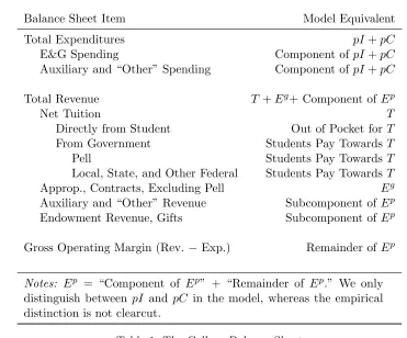
where p is the relative price of college expenditures, and Eg and Ep reflect the decomposition of non-tuition revenueE into public and private sources, respectively.1 Table1provides the mapping between model and data using institution-level IPEDS data from the Delta Cost Project.2
Balance Sheet Item Model Equivalent
Total Expenditures pI +pC
E&G Spending Component of pI +pC
Auxiliary and “Other” Spending Component of pI +pC
Total Revenue T+Eg+ Component ofEp
Net Tuition T
Directly from Student Out of Pocket for T From Government Students Pay TowardsT
Pell Students Pay TowardsT
Local, State, and Other Federal Students Pay TowardsT
Approp., Contracts, Excluding Pell Eg
Auxiliary and “Other” Revenue Subcomponent ofEp Endowment Revenue, Gifts Subcomponent ofEp
Gross Operating Margin (Rev. −Exp.) Remainder of Ep
Notes: Ep = “Component of Ep” + “Remainder of Ep.” We only distinguish between pI and pC in the model, whereas the empirical distinction is not clearcut.
Table 1: The College Balance Sheet
1
Empirically, we use the Higher Education Price Index (HEPI).
2The IPEDS data glossary can be found athttps://nces.ed.gov/pubs/web/fintab92.asp. Unfortunately, 7.5%
2.1 Trends
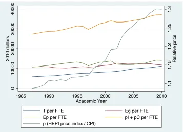
Figure 1 displays the path over time of the higher education price index p and each of the ma-jor spending and revenue categories, averaged across institutions using full-time equivalent (FTE)
enrollment weights. Notably, net tuition, expenditures, and the higher education price index demon-strate a clear upward trend. By contrast, the private component of non-tuition revenue has increased
only modestly, while public non-tuition revenue has remained almost completely flat.
1.1
1.15
1.2
1.25
1.3
R
e
la
ti
ve
p
ri
ce
0
10000
20000
30000
40000
2
0
1
0
d
o
lla
rs
1985 1990 1995 2000 2005 2010
Academic Year
T per FTE Eg per FTE
Ep per FTE pI + pC per FTE p (HEPI price index / CPI)
Figure 1: Trends in College Spending and Revenue
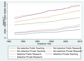
However, the average obscures wide variation in these patterns across college types. To delve deeper, figure 2 breaks down these trends by colleges’ degree of selectivity, research intensity, and status as either public or private. In absolute terms, net tuition has increased the most at selective,
private institutions, with public research institutions (regardless of selectivity) and non-selective private institutions not far behind. Non-selective, public teaching colleges have increased tuition
by the least amount. However, the tables turn when examined in percentage terms, and it is clear
that the rate of tuitioninflation has been highest at public institutions where attendance used to be more affordable. Table10 in AppendixA reports additional summary statistics by school type.
3
A Simplified Framework
0
5000
10000
15000
20000
25000
(me
a
n
)
T
1985 1990 1995 2000 2005 2010
Academic Year
Not selective Public Teaching Not selective Public Research Not selective Private Teaching Not selective Private Research Selective Public Research Selective Private Teaching Selective Private Research
Figure 2: Net Tuition By College Type
college and a unit measure of potential students. Students are distributed across academic abilityx
and parental incomey according to the densityf(x, y). Rather than provide explicit
microfounda-tions for college demand in this setup, we simply assume that students’ willingness to pay ist(x, y), which colleges can observe.
Suppose the college’s objective is to maximize “quality” q(X, I), which depends on average academic ability X and spending per student I. Because students always matriculate as long as
tuition does not exceed willingness to pay, the college sets student-specific tuition equal to t(x, y).
What remains is for the college to choose the measure of each student type to admit, α(x, y) ≤ f(x, y), taking into account how the resulting student body affects quality through peer effects and
the budget constraint. Specifically, the college solves
max
N >0,X,α(x,y)∈[0,f(x,y)]q(X, I)
s.t.pIN+pC(N) =EN + Z Z
t(x, y)α(x, y)dxdy
N =
Z
α(x, y)dxdy
X=
Z
xα(x, y)dxdy/N
(2)
costs, and p is the relative price of college goods. As in Epple et al. (2006), the college admits students for whom tuitiont(x, y) exceeds their “effective marginal cost,”
EM C(x, y)≡pI+pC0−E−pqX
qI
(x−X). (3)
The first three terms in (3) are the marginal resources spent when admitting an additional student, regardless of type. However, the last term states that high ability students are less costly
than low ability students because they contribute positively to the college’s quality.
For additional intuition, consider separating the college’s problem into two stages. The college
first decides on total enrollment N, and then the college selects who to admit. For given N, let
X(N) denote average academic ability and T(N) net tuition revenue per student. The college’s problem of choosing total enrollment N is given by
max
N >0q(X(N), I)
s.t.pIN+pC(N) =EN +T(N)N.
(4)
Assuming differentiability, the solution is characterized by the first order condition
qX
qI
X0(N) +1
pT
0(N) = d(C(N)/N)
dN . (5)
We can use this condition to generate predictions for how tuition responds to changing demand
and supply conditions.
3.1 Comparative Statics
Non-Tuition Revenue Condition (5) states that enrollment and net tuition are invariant to the amount of non-tuition revenue per student that the college receives. Therefore, the budget
constraint implies that changes in E pass through entirely to expendituresI.
Cost Changes The tuition impact of changing operating costs depends onhow C(N) shifts. For
example, ifC(N) is a polynomial, any change to the linear term acts exactly like an opposite shift in non-tuition revenue per student—namely, expenditures absorb the entire shift. By contrast, if
fixed costs increase, the term d(C(dNN)/N) falls. If the distributions of student academic ability and willingness to pay are independent, thenX(N) andT(N) are downward sloping (the college admits its best prospects first), in which case higher fixed costs prompt the college to increase enrollment
and reduce tuition.
alter marginal net tuition per student, T0(N), which implies that the college leaves enrollment unchanged, with higher expenditures absorbing the entire increase in tuition. However, if t(x, y) rises proportionally, colleges have the incentive to expand enrollment.
3.2 Summary and Limitations of the Simplified Framework
To summarize, the simplified framework delivers a few key predictions. First, higher non-tuition
revenue per student increases college expenditures, but not tuition or enrollment. Changes in linear costs have the same effect but in the opposite direction. Second, higher fixed costs induce the college
toincreaseenrollment at the expense of a less qualified student body and lower tuition revenues per student. Lastly, parallel shifts in student willingness to pay do not affect enrollment. The overall
takeaway is that careful attention must be paid not just to the sign but to the form of shifting
demand and supply conditions when assessing the likely impact on the higher education market. Nevertheless, this simplified framework is not suitable for quantitative analysis because of how
it abstracts from competition, general equilibrium effects, and richer student decision-making at
the extensive margins of whether/where to enroll in college and how to finance their education. To remedy these deficiencies, we turn to the full model.
4
The Quantitative Model
The quantitative model consists of heterogeneous, finitely-lived households, heterogeneous colleges, and the government.
4.1 Colleges
There is a finite numberK of college types, with each typek∈K representing a positive measure g(k) of identical colleges. Each college seeks to maximize quality, which depends positively on
aver-age academic ability, spending per student, and total enrollment (particularly in the case of public
colleges) while depending negatively on average parental income, as in Epple et al. (2006). School types differ exogenously along several dimensions, and additional heterogeneity arises endogenously
in equilibrium.
The first source of heterogeneity enters the college budget constraint, with colleges of type k receiving non-tuition revenue per student Ek and facing operating costsCk(N), where N is total enrollment. Next, colleges differ in terms of their student retention probabilities and post-graduation
labor market outcomes. Specifically, students attending college type kface an annual dropout risk of δk and earnings premia ofλk, both of which also depend on individual student ability.
us to analyze rich peer effects, sorting, and imperfect competition in equilibrium without the
addi-tional complications of strategic investment and dynamic market power. To be concrete, we first as-sume that colleges are subject to an annual balanced budget constraint. Instead of actively managing
an investment portfolio, colleges simply receive an exogenous flow of non-tuition revenue (which
in-cludes endowment earnings, direct government support, etc.) which supplements funds from endoge-nous tuition. Secondly, we assume that, after making admissions, tuition, and spending decisions
for each incoming cohort, colleges immediately trade the associated cash flows with a deep pocketed
intermediary that discounts at the rater. By implication, the college commits to keeping tuition and spending fixed for each cohort, and there is no cross-cohort subsidization. The expected stream of
payments for an incoming student of typesY isT(sY),(1−δk(sY))T(sY), . . . ,(1−δk(sY))JY−1T(sY),
where (1−δk(sY)) is the probability of retention. Definingω(sY) =PJj=1Y
(1−δk(sY))
1+r
j−1
, the net present value of these payments is T(sY)ω(sY). We assume that colleges similarly discount the
contribution of each student over time to each of the quality inputs.
Lastly, we introduce competitive search to allow for differential tuition pricing. In this setup,
student applicants and college vacancies are matched frictionally in submarketsm≡(T, sy) indexed
by tuition T and student characteristics sY. Each vacancy costs the college κ and is filled with
probability ρ(θ(m)), where θ(m) represents the market tightness, which the college takes as given.
With these assumptions, the college’s problem can be written as
max
v(m)≥0q(X, Y, I, N)
s.t. pIN+pC(N) +κ
Z
v(m)dm=
Z
T(m)ω(m)v(m)ρ(θ(m))dm+Eg(N) +Ep(N)
X=
Z
x(m)ω(m)v(m)ρ(θ(m))dm/N
Y =
Z
y(m)ω(m)v(m)ρ(θ(m))dm/N
N =
Z
ω(m)v(m)ρ(θ(m))dm
(6)
The interior solution states that, in active submarkets, tuition satisfies
T(m) = κ
ω(m)ρ(θ(m))
| {z }
Search premium
+pI+pC0(N)−Eg0(N)−Ep0(N)
| {z }
Common marginal cost
−pqN qI
N
| {z }
Size disc. −pqX
qI
(x−X)
| {z }
Ability discount
− pqY
qI
(y−Y)
| {z }
P. income penalty .
(7)
4.2 Households
Households go through three phases of life: youth, working age, and retirement.
4.2.1 Youth
Each period, a fixed measure of youths with heterogeneous characteristicssY = (x, y) consisting of
academic ability x and parental income y enter the economy at age j = 1 (corresponding to high school graduation). Youth choose between skipping college (k= 0) and attending one of the colleges
to which they receive admission,k∈K(sY). Collegekcharges type-specific net tuitionTk(sY) equal
to sticker priceTminus institutional aid, and students also face non-tuition expensesφ. Government grants ζ(Tk(sY) + φ, EF C(sY)) offset some of the cost of attendance, where EF C(sY) is the
expected family contribution formula that dictates eligibility for government need-based grants and
loans. The net cost of attendance comes out toN COAk(sY) =Tk(sY)+φ−ζ(Tk(sY)+φ, EF C(sY)).
While enrolled, college students receive additively-separable flow utility v(qk) which increases in college quality qk. To graduate, students must complete JY years of college. Students in class
j return to college each year with probability 1−δk(x) as long as j < JY; otherwise, they either
drop out or graduate. Students can borrow through the Federal Student Loan Program (FLSP).
The FSLP features subsidized loans that do not accrue interest while the student is in college,
where eligibility depends on financial need (N COA less EF C). Since 1993, students can borrow additional funds up to the net cost of attendance using unsubsidized loans.
Students face annual and aggregate limits for subsidized and combined borrowing given by ¯bj
and ¯l, respectively. Because students can borrow only up to the net cost of attendance, their annual combined subsidized borrowing bs and unsubsidized borrowing bu must satisfy
bs+bu≤min{b¯j, N COAk(sY)}. (8)
Similarly, define bsj as the statutory annual subsidized limit and lsj as the statutory aggregate subsidized limit. The actual amount that students can borrow in subsidized loans depends on their
net cost of attendance and the expected family contribution, both of which vary with student type. Apart from loans, students have two other means of paying for college. First, they have earnings
eY, which we treat as an endowment. Second, they receive a parental transferξEF C(sY), where
ξ∈[0,1] is a parameter. The budget constraint for a college student of type sY is
c+N COAk(sY)≤eY +ξEF C(sY) +bs+bu. (9)
4.2.2 Workers and Retirees
Working and retired households receive earnings that depend on their level of education, age/retirement
These households value consumption according to a period utility function u(c) and discount the
future at rate β. Workers with student loans face a loan interest rate of i and amortization pay-ments of p(l, t) =li(1+(1+ii))tt−1−1, where l represents the loan balance and tthe remaining duration. All
households can use a discount bond to save at the risk-free rater∗. For simplicity, we do not allow borrowing, although it could easily be incorporated. Workers who are delinquent on their loans face principal penalties and wage garnishment γ.
4.3 Value Functions
We assume the log of post-tax earnings, z, follows a random walk with innovations σ. Workers with student loans enter the period either in good standing or in a state of default and can choose
whether to maintain or switch their repayment status. In addition, workers make consumption and
saving decisions (we assume there is no borrowing outside of the student loan program). The value function for a worker who is not currently in default is
Vj(a, l, t, z, f = 0) = max{VjR+1(a, l, t, α), VjD+1(a, l(1 +η), z)}. (10)
where VR is the value of repayment and VD is the value of default. Defaulting borrowers are penalized with a proportional increaseη in their outstanding balance.
The value function for a worker who is currently in default is
Vj(a, l, z, f = 1) = max{VjR+1(a, l, tmax, α), VjD+1(a, l, z)} (11)
where loan rehabilitation resets the clock.
The value of choosing to make a payment is
VjR(a, l, t, z) = max
a0≥0u(c) +βEε0Vj+1(a
0
, l0, t0, z+σε0,0)
s.t.c+a0/(1 +r) +p(l, t)≤ez+µj+a
l0 = (l−p(l, t))(1 +i)
t0 = max{t−1,0}
(12)
The value of choosing to remain in default is
VjD(a, l, z) = max
a0≥0u(c) +βEε0Vj+1(a
0, l0, z+σε0,1)
s.t.c+a0/(1 +r) +γez+µj ≤ez+µj+a
l0 = max{0,(l−γez+µj)(1 +i)}
(13)
whereγ represents wage garnishment.
˜
Yj(l;z, δ, T, EF C) = max
c≥0,l0≥lu(c) +β(1−δ)1[j < JY] ˜Yj+1(l
0
;z, δ, T, EF C)
+βδEε0Vj+1
0, l0, tmax1[l0>0], z
j
JY + 1
+σ(j+ 1)1/2ε0,0
+β(1−δ1[j =JY])Eε0Vj+1(0, l0, tmax1[l0 >0], z+σ(j+ 1)1/2ε0,0)
s.t.c+T ≤eY +ξEF C+bs+bu+ζ(T+φ, EF C)
N COA=T+φ−ζ(T +φ, EF C)
bs=l0s−ls, bu=
l0u 1 +i−lu
bu ≤min{¯buj, N COA}, bs+bu ≤min{¯bj, N COA}
l0s+ l 0
u
1 +i ≤ ¯ l
(14)
where the decomposition of total loan balances into subsidized/unsubsidized components is
(l0s, l0u) = (
(l0,0) ifl0 ≤˜lsj(N COA, EF C)
(˜lsj(N COA, EF C), l0−˜lsj(N COA, EF C)) otherwise
(ls, lu) =
(
(l,0) ifl≤˜ljs−1(N COA, EF C)
(˜ls
j−1(N COA, EF C), l−l˜sj−1(N COA, EF C)) otherwise.
(15)
Note that the college premium z, drop out rate δ, and tuition T are all state variables. In this specification, the college earnings premium gradually increases with each year of enrollment, and
there is a discrete jump upon graduation to reflect the sheep-skin effect.
The value of attending college k (net of preference shocks) is then
Yk(T, sY) = ˜Y1(0;λk(sY) +ν+ log(1−τ), δk(sY), T, EF C(sY)) (16)
The value of not attending college is defined as
Y0(T, sY) =Eε0V1(0,0,0, σε0,0). (17)
Youths expect a probability η(θ(m)) of being accepted to a school conditional on entering
submarketm= (T, sy). For tractability, we assume that youth only submit one college application,
but they can adjust search intensitysto increase their probability of acceptance. Exerting intensity
s ≥ 1 in submarket m leads to a match with probability min{sη(θ(m)),1} and creates search disutility αs(s−1)σs with σs > 1. In fact, we go further and assume youths only choose (m, s)
combinations that lead to college acceptance with probability 1.3
3
Conditional on applying to college k, the youth’s choice of submarket m solves
max
i≥1,m∈M(sY)
min{sη(θ(m)),1}(Yk(m)−Y0(m)) +Y0(m)−ψ(i−1)2
s.t.iη(θk(m)) = 1
(18)
where k = 0 represents the decision to skip college. Thus, the value of applying to college k and submarketm∈M(sY) with intensityi= 1/η(θ(m)) is
max
k∈{0,...,K},m∈M(sY)
Yk(m)−ψ(1/η(θk(m))−1)2 (19)
To these, we add idiosyncratic preference shocks that allow for unobserved preferences for
colleges:
max
k∈{0,...,K},m∈M(sY)
Yk(m)−ψ(1/η(θk(m))−1)2+ 1
αε
k,α >0. (20)
Breaking this into two parts, define
ˆ
Yk(sY) := max
m∈M(sY)
Yk(m)−ψ(1/η(θk(m))−1)2 (21)
with policy function mk(sY) and
max
k∈{0,...,K} ˆ
Yk(sY) +
1
σε
k. (22)
Assuming these shocks are distributed according to a Type 1 extreme value distribution, the probability of applying to schoolk is
Ak(sY) :=
exp(σ( ˆYk(sY)−Yˆ0(sY))))
PK
˜
k=0exp(σ( ˆY ˜
k(s
Y)−Yˆ0(sY)))
. (23)
Because we assume that applicants (conditional on apply to k) exert enough search effort to go with probability 1, this is also the enrollment rate for typesY.
The effective search exerted by student typesY for school typekisf(sY)Ak(sY)/η(θk(mk(sY))).
The total number of vacancies, assuming that the measure of each school type isg(k), isg(k)v(mk(sY)).
So, the implied market tightness in each submarket is
θk(m) =
( η(θk(mk(s
Y))g(k)v(mk(sY))
f(sY)Ak(sY) ifsY is such that m=m
k(s Y)
0 otherwise . (24)
4.4 Government
The government levies proportional taxes on labor earnings to fund transfers and loans (subsidized
and unsubsidized) to students in college. Other sources of revenue for the government include
interest payments on unsubsidized loans for students in college as well as loan payments and garnishment from workers with outstanding student loans.
4.5 Equilibrium
A steady state equilibrium consists of market tightnesses θk(sY), college policies Xk, Ik, Nk, vk,
value functions Yk and V, application rates Ak, and tax rates such that
1. Colleges optimally choose their policies taking market tightnesses as given;
2. students and workers optimize taking market tightnesses and tax rates as given;
3. application ratesAkand market tightnessesθkare consistent with the student value function Yk and vacancy creation vk; and
4. the government balances its budget.
5
Calibration and Estimation
5.1 Mapping the Model to the Data
One unit of the consumption good is treated as $1,000 in 2010 dollars. We take ability to be U[0,1]. We assume that N in the data is a school’s FTE share times the enrollment rate. Table 2 summarizes how we map the data and model populations.
Data Model
Youth population 1
Number of schools within each type g(k) A school’s FTE share ×the enrollment rate N
Table 2: Mapping between the data and model
5.2 College Quality
We assume q is given by a CES quality function
q(X, Y, I, N) =αXX
−1
+αYY− −1
+αII −1
+αNN −1
−1
where≥0 is the elasticity of substitution. Note thatY is a “bad” in that its exponent is−(−1)/.4 The Cobb-Douglas case is the limiting case of = 1, perfect complements is the limiting case of = 0, and perfect substitutes is the limiting case of =∞.
Note that the model has extremely tight predictions about net tuition for each student, but
it is totally silent as to “sticker price” tuition. To overcome this and allow sticker prices in the data to help discipline the quality function parameters, we construct an artificial sticker price
in the model as follows. IPEDS / DCP has two relevant measures of tuition discounts. One is
the percent of students receiving institutional grants and the other is the average amount of the institutional grant. Using the first measure, we construct a cutoff T such that P(T ≤ T) is the fraction receiving institutional grants. We then take E(T|T >T) as the “sticker price.” We take E(T|T > T)−E(T|T ≤ T) as the average institutional grant. With E(T|T > T) as the sticker
price and net tuition as E(T), we can then match the discounts.
We note that for the solution to an individual college problem, the overall returns to scale in the
college quality function is irrelevant if there is no feedback from college quality to student demand. (This is because any monotone transformationQwill result in the same solution.) So we normalize
αX to 1.
5.3 Non-Tuition Revenue and Operating Costs
For the functional forms of Eg(N) and Ep(N) we use linear specifications Eg(N) = Eg,kN and Ep(N) =Ep,kN as this should give results close to what is seen in the data.
Following Epple et al.(2006), we posit operating costs of the form
C(N) =ck0 +c1kN+ck2N2. (26)
Rather than try to calibrate 3K parameters, we make some assumptions that help match college
sizes using information from a “nearby” problem. First, we assume that ck1 = 0 for all k. We then consider the solution to (5) under the assumption that there is no student heterogeneity and consequently X0(N) and T0(N) are zero after allowing for quality to depend on N. The FOC becomes
qN
qI
+1 p
d(E(N)/N)
dN =
d(C(N)/N)
dN (27)
whereqN/qI is (αN/αI)(N/I)−1/. To calibrate, we assume that enrollments observed in the data
correspond to the efficient scale, and by that we mean the solution to this problem. In other words,
4
Because of numerical precision issues, we scaleN so thatαN reported later in the paper is theαN here times
Nk=N and the FOC satisfies
ck2(Nk)2 =ck0+αN αI
Nk
I
!−1/
(Nk)2 (28)
If one knewI, the right hand andNk are either parameters or taken from the data. Consequently, this equation would pin down ck0 as a function of ck2 (or vice-versa) for each k. We proxy for I by assuming it is two-thirds of the observed average expenditures per FTE in the data Sk, i.e., Ik = 231pSk. This still gives K remaining cost parameters. To discipline this, we assume that the fixed cost is a proportion c∈[0,1] of total expenditures in the data,
ck0 =c1
pS
k
Nk (29)
where Sk denote the observed average expenditures per FTE in the data. Thus we are left with just one free parameter, c.
5.4 Matching Technology
We assume a CES matching function for vacancies v and intensity-adjusted applicants ˜u=iuis
m(˜u, v) = ˜umin
A(v/u˜) (1 + (v/u˜)γ)1/γ,1
(30)
The resulting matching rate for intensity-adjusted applicants,η(θ) = m(˜uu,v˜ ), is
η(θ) = min
Aθ (1 +θγ)1/γ,1
and ρ(θ) = η(θ)
θ (31)
where θ = v/u˜ is the market tightness. We take γ = 1 and then choose A so that when θ = 1,
students and colleges match with a 95% probability, i.e., A= 2·.95.
5.5 Dropout Risk and Earnings Premia
Graduation rates and college premiums vary greatly by school, as does our measure of average ability of the student body. We assume that these depend partially on individual ability and partially on
school type. In order to almost exactly match the data without over-burdening the estimation,
we assume a constant split µ between an individual’s contribution and the school’s contribution. Specifically, for continuation rates we assume
(1−δk(x)) = min{max{(1−δk)(µδ+ (1−µδ)
x
whereδk is from the data,x is individual ability, andXk is average ability (at school k).
To determine an appropriate value forµ, we turn to the data. First, we construct sticker tuition quintiles as a proxy for college types. Then, within these quintiles we compute average ability
and average graduation rate. Then we regress graduation on a quintile dummy times the average graduation rate times the individual’s ability over average ability. The results are presented in Table
18 in the appendix. Interestingly, the lowest quintile has no statistically significant relationship between ability and graduation. However, the other quintiles seem to have a significant and stable relationship with coefficients around 40%. Consequently, we take µ = .6 to generate something
close to this.
Similarly, we take the relative college premium as
λk(x) =λk(µλ+ (1−µλ)
x
Xk) (33)
and the follow the same procedure as above but using the log college premium in placed of the
graduation dummy. The results are also in Table 18. The results seem relatively stable across the quintiles, and we set µλ = .1. Note that these estimates do not say that the college premium is
nearly similar across schools. In fact, using the NLSY97 data we find the log college premium for the
lowest quintile is .363 while the highest quintile is .643, a .28 log point difference or approximately 32.3%.
5.6 Parental Transfers
To calibrate ξ, which determines parental transfers ξEF C(sY), we use NLSY97 data. First, we
compute parental income and then apply the EFC formula fromEpple et al.(2013) to get an EFC measure. Then we use data on family aid for college that is not expected to be paid back and find
the annual level of support. We then regress this transfer measure on interactions of EFC with graduating and not graduating (we exclude a constant since the model lacks one). The results are
given in Table3. Transfers end up higher for dropouts, which may reflect many things such as the family’s resources being exhausted over time. We setξ= 0.7 as our primary object of interest and the preference shock can somewhat account for these differences in transfers.
5.7 Jointly Estimated Parameters
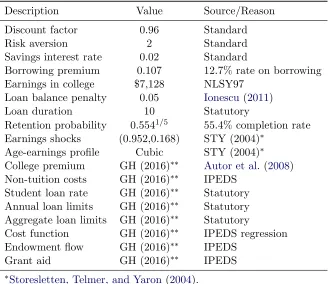
Currently, the calibration and to some extent the model are still in flux. Table 4 summarizes most of the calibration of the non-college-specific parameters. The remaining free parameters are
jointly estimated to fit a large number of moments including net and sticker tuition at each school,
enrollment shares, expenditures, enrollment rates, ability at each school, and the correlation between parental income and enrollment. These parameters are summarized in Table 5.
(1) (2) Family grant Family grant
Dropped out×EFC (real) 0.0939∗∗∗ 0.419∗∗∗ (6.70) (4.46)
Graduated×EFC (real) 0.185∗∗∗ 0.901∗∗∗ (27.31) (30.16)
Observations 2063 771
R2 0.277 0.547
tstatistics in parentheses
(1) is the full sample; (2) includes only those with EFC<net tuition.
∗
p < .1,∗∗ p < .05,∗∗∗p < .01
Table 3: Transfers as a function of EFC
Description Value Source/Reason
Discount factor 0.96 Standard
Risk aversion 2 Standard
Savings interest rate 0.02 Standard
Borrowing premium 0.107 12.7% rate on borrowing Earnings in college $7,128 NLSY97
Loan balance penalty 0.05 Ionescu (2011)
Loan duration 10 Statutory
Retention probability 0.5541/5 55.4% completion rate Earnings shocks (0.952,0.168) STY (2004)∗
Age-earnings profile Cubic STY (2004)∗ College premium GH (2016)∗∗ Autor et al. (2008) Non-tuition costs GH (2016)∗∗ IPEDS
Student loan rate GH (2016)∗∗ Statutory Annual loan limits GH (2016)∗∗ Statutory Aggregate loan limits GH (2016)∗∗ Statutory
Cost function GH (2016)∗∗ IPEDS regression Endowment flow GH (2016)∗∗ IPEDS
Grant aid GH (2016)∗∗ IPEDS ∗Storesletten, Telmer, and Yaron (2004).
∗∗Web appendix A ofGordon and Hedlund(2016).
Description Parameter Value
Preference shock size σ 8.062
Search effort level ψ 1000.000
Cost parameter c 0.001
Quality’s elasticity 0.525
Quality’s weight on investment αI 31.805
Quality’s weight on enrollmentN, public schools αgN 0.133 Quality’s weight on enrollmentN, private schools αpN 0.088 Quality’s weight on inverse parental incomeY−1 αY 0.012
Table 5: Jointly estimated parameters
graphically. This is done in Figure3. Each blue dot represents a particular type of school with the vertical position giving the data’s moment and the horizontal positive giving the model’s moment. If the model had perfect predictions, all the blue dots would lie on the 45-degree line. We have
also labeled the school type that gives the worst fit among the seven school types. For instance,
the worst fit for net tuition comes from GRS where G stands for public, R stands for research, and S stands for selective. Similarly, the worst for FTE share comes from PTN which is private (P),
teaching (T), nonselective (N) schools. Overall, it seems the model does a fair job of matching the
targeted moment with some noteworthy exceptions.
0 5 10 15 20
Model 0 10 20 Data Net tuition GRS
0 10 20 30
Model 0 10 20 30 Data Sticker price GRS
0 20 40 60 80
Model 0 50 100 Data Expenditures GRS
0 0.1 0.2 0.3 0.4
Model 0 0.2 0.4 Data FTE share GTN
0.2 0.4 0.6 0.8 1
Model 0 0.5 1 Data Relative ability PRN
50 100 150 200
Model 50 100 150 200 Data Parental income PTS 45 deg Model vs. data
Figure 4shows equilibrium heat maps for enrollment in 1987 across the 7 college types and the decision to skip college. The calibration gives that research-intensive and selective colleges are more likely to attract high ability students, and this sorting is starker at private institutions. By contrast,
low ability students disproportionately skip college entirely, regardless of parental income. Students
coming from the lowest income families almost never attend selective private colleges, no matter their academic ability. Instead, such students either attend selective public research institutions or
non-selective institutions.
No college
0 0.5 1 0 50 100 150 200 Parental income GTN
0 0.5 1 0 50 100 150 200 GRN
0 0.5 1 0 50 100 150 200 PTN
0 0.5 1 0 50 100 150 200 PRN
0 0.5 1
Ability 0 50 100 150 200 Parental income GRS
0 0.5 1
Ability 0 50 100 150 200 PTS
0 0.5 1
Ability 0 50 100 150 200 PRS
0 0.5 1
Ability 0 50 100 150 200
Figure 4: Sorting in 1987
6
Results
We break the results discussion into three parts. First, we describe how we change parameters of the model to capture the theories. Second, we allow all factors to change simultaneously to bring
the benchmark (1987) model to the terminal steady state (2010). This serves as model validation.
Third, we run counterfactuals and decompose the importance of relative factors by allowing only some to change.
6.1 Implementing the Theories
• For Baumol cost disease, we increasepby the same amount that the Higher Education Price Index / CPI increased from 1987 to 2010.
• For the “macroeconomic forces” driven demand changes,
– we increase the average college premium λby an amount consistent with the 1987-2010
change reported inAutor et al.(2008) (extrapolating slightly to reach 2010 as described inGordon and Hedlund,2016);
– we increase the expected family contribution EF C(sY) as if the parental income had
increased from 69.3% of its 2010 value to its 2010 value, which is consistent with the increase in the real GDP per capita from 1987 to 2010 (roughly a 1.3% annual growth
rate);5
– and we move the college completion rates from their 2002 value (the earliest year for
which we have data on this series from IPEDS/DCP) to their 2010 value.
• For the Bennett story (colleges capturing financial aid),
– we change the Federal Student Loan Program borrowing limits according to the statutory
values (including the introduction of unsubsidized loans beginning in 1993);
– we change real interest rates on student loans according to the statutory limits (and we average over the 10 year repayment period as described inGordon and Hedlund,2016);
– we increase φ(the non-tuition expenses of attending college), which increases eligibility
for subsidized student loans, according to the estimates of these costs reported by NCES; and
– we increase mean Pell grants according the mean value reported by NCES.
• For the public and private non-tuition revenue stories, we change the average per student values (Eg,k,Ep,k) according to the value in IPEDS/DCP.
6.2 Model Validation
Because of the large number of moments, we again resort to a graph (Figure5) to assess the model’s performance at matching untargeted moments over time. The horizontal position of the solid circle (a “cannonball”) represents the model’s prediction for 2010 and the vertical position represents
the data’s value in 2010. Opposite the cannonball are the values for 1987. If the model perfectly
captures the data, all the cannonball trajectories would lie on top of the 45 degree line. However, if the trajectories are parallel to the 45 degree line, then the model would exactly predict the changes.
5
Qualitative failures of the model have trajectories that are orthogonal to the 45 degree. Overall,
the model seems to do very well at matching the untargeted changes in net tuition, expenditures, ability, and enrollment correct (as we do not have parental income for 1987, we cannot construct
the graph for it).
0
20
40
Model
0
20
40
Data
Net tuition
0
20
40
60
Model
0
50
Data
Sticker price
0
50
100
150
Model
0
50
100
150
Data
Expenditures
0.2
0.4
0.6
0.8
Model
0
0.5
1
Data
Relative ability
0
0.1
0.2
Model
0
0.1
0.2
Data
Enrollments 45 degree
GTN GRN PTN PRN GRS PTS PRS
Figure 5: Data vs. model predictions, 1987-2010
6.2.1 Empirical Evidence on Tuition Discounting
Table 6 provides some empirical evidence that colleges discount tuition based on both ability and parental income. Appendix B reports similar results broken out by ability decile, as well as additional regressors of net tuition or sticker tuition.
6.3 Decomposing the Importance of Relative Factors
Given that the model successfully replicates the overall rise in net tuition between 1987 and 2010,
Discount (% off)
Ability 7.472∗∗
Parental income in 1996 (real) -0.0972∗∗∗
Constant 34.15∗∗∗
Observations 1609
R2 0.047
∗
p < .1,∗∗ p < .05,∗∗∗ p < .01
Table 6: Tuition discounting
steps. First, we looking at the factors’ impacts on FTE-weighted values. Second, we look at the heterogeneous impact across schools.
6.3.1 Average Impacts Across Schools
Table 7 displays how much each of the theories can individually and jointly explain the increase in net tuition. The “% Expl.” columns give the percentage of the data’s change explained by the model. Overall, the theories can jointly account for the entire net tuition increase. However, the bulk
of the increase comes from the demand side, predominantly the non-policy-driven ones resulting
from a higher college earnings premium, lower dropout rates, and higher parental income. On their own, these explain 76% of the increase. The Bennett theory also accounts for 42% of the increase
in net tuition. Baumol cost disease plays only a small role, accounting for 7% of the increase in
net tuition. The other theories that focus on cuts in public support or changes private non-tuition revenue contribute nothing: The model predicts they would have acted to decrease net tuition on
their own. All the theories drive up expenditures, albeit to varying degrees. The model predicts the
largest contributor to be private non-tuition revenue.
Net tuition Expenditures
Experiment Model Data % Expl. Model Data % Expl.
1987 5.8 5.8 0 27.3 27.4 0
1987+Baumol (p) 6.2 - 7 27.6 - 3
1987+Demand (λ,δ) 9.9 - 76 30.8 - 36
1987+Bennett 8.1 - 42 29.4 - 22
1987+Pub. rev. (Eg) 5.5 - -6 29.2 - 20
1987+Priv. rev. (Ep) 4.6 - -23 32.2 - 51
2010 (1987+everything) 11.6 11.2 108 40.1 37.1 132
Net Tuition
% = 178 % = 46
% = 170 % = 77
% = 43 % = 87 % = 79
-100 -50 0 50 100 150 200 250 300 350 GRN GRS GTN PRN PRS PTN PTS Expenditures
% = 35
% = 54 % = 32
% = 31
% = 58 % = 24
% = 60
-20 -10 0 10 20 30 40 50 60 70
GRN GRS GTN PRN PRS PTN PTS Enrollment
% = 33
% = 48 % = 32
% = 32
% = 57 % = 27
% = 63
-20 -10 0 10 20 30 40 50 60 70
GRN GRS GTN PRN PRS PTN PTS Relative ability
% = -0 % = -0
% = -1 % = -6 % = -1
% = -4 % = -5
-10 0 10 20
GRN GRS GTN PRN PRS PTN PTS
6.3.2 Empirical Evidence on the Impact of Government Support
We now look at how non-tuition revenue influences tuition, expenditures, and enrollment in the
data. The first column of the top panel of table8reveals strong cross-sectional relationship between tuition and non-tuition revenue per FTE. In particular, public support (Eg) per FTE is negatively correlated with net tuition (T); in contrast, private non-tuition revenue (Ep) is positive correlated with net tuition. However, after controlling for interactions between state, school type, and flagship
status, these correlations disappear as can be seen in the second column. This is also true if one expands from just 1987 to 2010 provided one all has interactions with time dummies as can be seen
in the third column, or with a fixed effects specification like in the fourth column.
6.3.3 Heterogeneous Impacts Across Schools
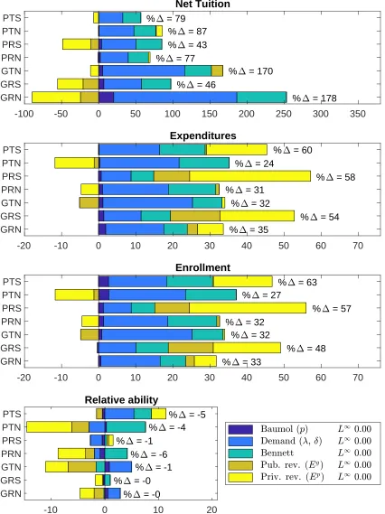
Figure 6 presents the tuition decomposition first by implementing the forces one at a time. (For beginning at 2010 and removing one force at a time, one may consult Figure 8 in the appendix.) Each panel represents a different variable of interest with net tuition in the top panel. The horizontal
axis gives percent change, the vertical axis gives different school types. The %∆ gives the overall percent change induced on net tuition from all the forces. A given bar shows the percent change
from a particular force. For instance, the light blue represents the change induced by “Demand,
λ, δ”—i.e., only letting the non-policy demand forces change. For GRN, this force alone would have increased net tuition by around 160%, while for PRN it would have done so by around 40%.
The main drivers of net tuition increases are the demand side changes, both the policy-induced
ones (Bennett) and the macroeconomic forces (Demand, λ, δ). Moreover, this seems to be pretty robust across school types despite wildly different endowments and student bodies. Baumol seems to
have increased net tuition only slightly. The model predicts that non-tuition revenue acted mostly to decrease net tuition.
The model also has predictions for variables other than net tuition, and we briefly discuss them.
Almost all the theories serve to increase expenditures. In contrast to the simple model, demand has a significant impact on enrollment. This is a consequence of the college quality function directly
incorporating enrollment in the college quality function. For most schools, changes in non-tuition
revenue have acted to reduce ability and increase enrollment.
7
Conclusion
The model results indicate that demand-side changes are driving most of the net tuition increases.
The bulk of this is driven by non-policy-induced demand changes, but policy-induced demand changes also play a large role. Despite the substantial 20% increase in relative costs of college
(1) (2) (3) (4)
T T T T
Eg -0.26∗∗∗ -0.04∗ -0.01 0.02
Ep 0.09∗∗∗ 0.00 -0.00 -0.00
Constant 13266.80∗∗∗ 12949.12∗∗∗ 9904.17∗∗∗ 7399.60∗∗∗
Observations 1158 1158 27792 27792
Adjusted R2 0.149 0.727 0.750 0.463
(1) (2) (3) (4)
XPND XPND XPND XPND
Eg 0.74∗∗∗ 0.96∗∗∗ 0.99∗∗∗ 1.02∗∗∗
Ep 1.09∗∗∗ 1.00∗∗∗ 1.00∗∗∗ 1.00∗∗∗
Constant 13266.80∗∗∗ 12949.12∗∗∗ 9904.17∗∗∗ 7399.60∗∗∗
Observations 1158 1158 27792 27792
Adjusted R2 0.980 0.994 0.994 0.974
(1) (2) (3) (4)
log(N) log(N) log(N) log(N)
log(Eg) 0.40∗∗∗ -0.05 -0.05∗∗∗ -0.06∗∗∗ log(Ep) -0.14∗∗∗ -0.15∗∗∗ -0.19∗∗∗ -0.12∗∗∗ Constant 6.37∗∗∗ 9.89∗∗∗ 10.08∗∗∗ 9.33∗∗∗
Observations 1105 1105 26721 26721
Adjusted R2 0.366 0.711 0.718 0.463
(1) (2)
Ability Ability
log(Eg) 0.01∗ -0.01
log(Ep) 0.14∗∗∗ 0.06∗∗∗ Constant -0.95∗∗∗ -0.13
Observations 931 931
Adjusted R2 0.300 0.611
References
B. Abbott, G. Gallipoli, C. Meghir, and G. Violante. Education policy and intergenerational
transfers in equilibrium. Mimeo, 2016.
R. J. Andrews, J. Li, and M. F. Lovenheim. Quantile treatment effects of college quality on earnings: Evidence from administrative data in texas. Mimeo, 2012.
R. B. Archibald and D. H. Feldman. Explaining increases in higher education costs. The Journal
of Higher Education, 79(3):268–295, 2008.
K. Athreya and J. Eberly. Risk, the college premium, and aggregate human capital investment.
Mimeo, 2016.
D. H. Autor, L. F. Katz, and M. S. Kearney. Trends in U.S. wage inequality: Revising the
revi-sionists. The Review of Economics and Statistics, 90(2):300–323, May 2008.
W. J. Baumol. Macroeconomics of unbalanced growth: The anatomy of urban crisis. The American Economic Review, 57(3):415–426, 1967.
W. J. Baumol and W. G. Bowen. Performing Arts: The Economic Dilemma; a Study of Problems
Common to Theater, Opera, Music, and Dance. Twentieth Century Fund, 1966.
P. Belley and L. Lochner. The changing role of family income and ability in determining educational
achievement. Journal of Human Capital, 1(1):37–89, 2007.
D. Card and T. Lemieux. Can falling supply explain the rising return to college for younger men?
Quarterly Journal of Economics, 116:705–746, 2001.
S. R. Cellini and C. Goldin. Does federal aid raise tuition? new evidence on for-profit colleges. American Economic Journal: Economic Policy, 6:174–206, 2014.
R. Chakrabarty, M. Mabutas, and B. Zafar. Soaring tuitions: Are public
fund-ing cuts to blame? http://libertystreeteconomics.newyorkfed.org/2012/09/
soaring-tuitions-are-public-funding-cuts-to-blame.html#.VeDDrPlVhBc, 2012. Ac-cessed: 2015-08-28.
S. Chatterjee and F. Ionescu. Insuring student loans against the risk of college failure. Quantitative Economics, 3(3):393–420, 2012.
A. F. Cunningham, J. V. Wellman, M. E. Clinedinst, J. P. Merisotis, and C. D. Carroll. Study
of college costs and prices, 1988 - 89 to 1997 - 98, volume 1. Report NCES 2002-157, National
A. F. Cunningham, J. V. Wellman, M. E. Clinedinst, J. P. Merisotis, and C. D. Carroll. Study of
college costs and prices, 1988 - 89 to 1997 - 98, volume 2: Commissioned papers. Report NCES 2002-157, National Center for Education Statistics, 2001b.
D. Epple, R. Romano, and H. Sieg. Admission, tuition, and financial aid policies in the market for
higher education. Econometrica, 74(4):885–928, 2006.
D. Epple, R. Romano, S. Sarpca, and H. Sieg. The U.S. market for higher education: A general equilibrium analysis of state and private colleges and public funding policies. Mimeo, 2013.
I. Fillmore. Price discrimination and public policy in the U.S. college market. Mimeo, 2016.
A. B. Frederick, S. J. Schmidt, and L. S. Davis. Federal policies, state responses, and community
college outcomes: Testing an augmented bennett hypothesis. Economics of Education Review,
31(6):908–917, 2012.
C. Fu. Equilibrium tuition, applications, admissions, and enrollment in the college market. Journal
of Political Economy, 122(2):225–281, 2014.
C. Garriga and M. P. Keightley. A general equilibrium theory of college with education subsidies,
in-school labor supply, and borrowing constraints. Mimeo, 2010.
C. Goldin and L. F. Katz. The race between education and technology: The evolution of u.s.
educational wage differentials, 1890 to 2005. NBER Working Paper, 2007.
G. Gordon and A. Hedlund. Accounting for the rise in college tuition. Working Paper 21967,
NBER, 2016.
D. E. Heller. The effects of tuition and state financial aid on public college enrollment. The Review of Higher Education, 23(1):65–89, 1999.
L. Hendricks and O. Leukhina. The return to college: Selection bias and dropout risk. Mimeo,
2016.
M. Hoekstra. The effect of attending the flagship state university on earnings. The Review of Economics and Statistics, 91(4):717–724, 2009.
F. Ionescu. Risky human capital and alternative bankruptcy regimes for student loans. Journal of
Human Capital, 5(2):153–206, 2011.
J. B. Jones and F. Yang. Skill-biased technological change and the cost of higher education. Journal of Labor Economics, 34(3), 2016.
L. F. Katz and K. M. Murphy. Changes in relative wages, 1963 - 87: Supply and demand factors.
M. P. Keane and K. I. Wolpin. The effect of parental transfers and borrowing constraints on
educational attainment. International Economic Review, 42(4):1051–1103, 2001.
R. K. Koshal and M. Koshal. State appropriation and higher education tuition: What is the
relationship? Education Economics, 8(1), 2000.
L. J. Lochner and A. Monge-Naranjo. The nature of credit constraints and human capital.American
Economic Review, 101(6):2487–2529, 2011.
B. T. Long. How do financial aid policies affect colleges? the institutional impact of the georgia hope scholarship. Journal of Human Resources, 39(4):1045–1066, 2004a.
B. T. Long. The impact of federal tax credits for higher education expenses. In C. M. Hoxby, editor, College Choices: The Economics of Where to Go, When to Go, and How to Pay for It,
pages 101 – 168. University of Chicago Press, 2004b.
B. T. Long. College tuition pricing and federal financial aid: Is there a connection? Technical
report, Testimony before the U.S. Senate Committee on Finance, 2006.
D. O. Lucca, T. Nadauld, and K. Shen. Credit supply and the rise in college tuition: Evidence from expansion in federal student aid programs. Mimeo, 2015.
M. S. McPherson and M. O. Shapiro. Keeping College Affordable: Government and Educational Opportunity. Brookings Institution Press, 1991.
M. J. Rizzo and R. G. Ehrenberg. Resident and nonresident tuition and enrollment at flagship state
universities. In C. M. Hoxby, editor,College Choices: The Economics of Where to Go, When to Go, and How to Pay for It, pages 303 – 353. University of Chicago Press, 2004.
L. D. Singell, Jr. and J. A. Stone. For whom the Pell tolls: The response of university tuition to federal grants-in-aid. Economics of Education Review, 26:285–295, 2007.
K. Storesletten, C. Telmer, and A. Yaron. Cyclical dynamics in idiosyncratic labor market risk.
Journal of Political Economy, 112(3):695–717, 2004.
M. A. Titus, S. Simone, and A. Gupta. Investigating state appropriations and net tuition revenue for
public higher education: A vector error correction modeling approach. Working paper, Institute for Higher Education Law and Governance Institute Monograph Series, 2010.
L. J. Turner. The road to Pell is paved with good intentions: The economic incidence of federal student grant aid. Mimeo, 2013.
N. Turner. Who benefits from student aid: The economic incidence of tax-based aid. Economics of
A
Detailed Data Sources and Description
A.1 IPEDS/DCP data
A.2 NLSY 97 Data
B
Additional Results
B.1 Empirical Results
Balance sheet item Model equivalent DCP variable
Total Expenditures pI+pC eandg01 sum +
auxother cost E&G spending** Part of pI+pC eandg01 sum
E&R spending pI
Instruction Part of pI+pC instruction01
Research Part of pI+pC research01
Public service Part of pI+pC pubserv01 Academic support Part of pI+pC acadsupp01 Student services Part of pI+pC studserv01 Institutional support Part of pI+pC instsupp01 Plant operation / maintenance Part of pI+pC opermain01
Scholarships and fellowships Part of pI+pC grants01,grants01 fasb Auxiliary and “other” spending Part of pI+pC auxother cost
Total Revenue T+Eg+part of Ep tot rev w auxother sum
Net tuition T nettuition01 −
grants01
Directly from student Out of pocket for T net student tuition From government Students apply to T nettuition01
-net student tuition
Pell Students apply to T grant01
Local, state, and other federal Students apply to T nettuition01 -net student tuition - grant01
Approp., contracts, excluding Pell Eg state local app +
state local grant contract
+
fed-eral10 net pell* Auxiliary and “other” revenue Part of Ep auxother rev Endowment revenue, gifts Part of Ep priv invest endow
Gross operating margin (rev. - exp.) Part of Ep tot rev w auxother sum eandg01 sum -auxother cost
Note:Ep is the sum of “Part ofEp” andpC is the sum of “Part ofpC.”
*Computed as a residual: tot rev w auxother sum - nettuition01 - priv invest endow - auxother rev **A component of E&G spending is expenditures on scholarships and fellowships with the definition varying over time. Because of reporting changes, we cannot subtract this off in a consistent way, so we leave it. Post 1997 for FASB institutions and 2002 for GASB it should reflect expenses from administering scholarships and fellowships.
1987 financial measures and shares
School type T Expend Eg Ep FTE share
Public, Teaching, Non-selective 2.7 14.9 9.2 3.0 0.25 Public, Research, Non-selective 3.7 25.9 13.7 8.5 0.36 Private, Teaching, Non-selective 9.6 19.9 1.4 9.0 0.15 Private, Research, Non-selective 11.9 27.0 3.8 11.3 0.05
Public, Research, Selective 4.0 39.5 21.3 14.3 0.10
Private, Teaching, Selective 14.3 32.6 1.0 17.3 0.01 Private, Research, Selective 15.5 72.2 14.1 42.7 0.08
2010 financial measures and shares
School type T Expend Eg Ep FTE share
Public, Teaching, Non-selective 6.4 17.8 7.9 3.5 0.25 Public, Research, Non-selective 8.8 35.5 14.9 11.8 0.35 Private, Teaching, Non-selective 15.1 22.5 1.1 6.3 0.18 Private, Research, Non-selective 20.3 34.0 4.1 9.6 0.05 Public, Research, Selective 10.0 65.3 29.1 26.2 0.09 Private, Teaching, Selective 24.3 50.0 1.2 24.5 0.01 Private, Research, Selective 23.7 115.4 22.0 69.6 0.07
Additional 2010 measures
School type Rel. premium Comp. rate P. inc. Rel. X # schools
Public, Teaching, Non-selective 0.83 0.47 53 0.26 242 Public, Research, Non-selective 0.95 0.58 65 0.48 129 Private, Teaching, Non-selective 0.89 0.58 71 0.34 639 Private, Research, Non-selective 1.08 0.65 81 0.51 50
Public, Research, Selective 1.19 0.73 77 0.90 20
Private, Teaching, Selective 1.29 0.89 110 0.94 36
Private, Research, Selective 1.63 0.87 91 0.96 42
Note: Monetary values are in 2010 dollars deflated using the CPI.
(1) (2) (3) (4) (5) (6)
Mean Mean Mean Mean Mean Mean
Enrolled 0.428 1 1 0.460 1 1
Graduated 0.300 0.714 1 0.325 0.719 1
Years college 1.628 3.867 4.488 1.779 3.919 4.535
Sticker tuition estimate (real) 14.10 16.08 14.33 16.29 Net tuition estimate (real) 8.792 10.16 8.933 10.22
Family transfers (real) 3.657 4.588 3.641 4.481
Grants (school or gov.) (real) 5.311 5.920 5.401 6.069 Loans (private or gov.) (real) 3.197 3.515 3.301 3.647
Took out a loan 0.560 0.604 0.587 0.634
Ability 0.506 0.677 0.709
Household income in 1996 (real) 73.37 92.71 99.10
EFC (real) 10.86 15.48 17.04
Observations 6536 2616 1868 4102 1778 1278
Note: All estimates are means from the NLSY97 data, unweighted using the cross-section sample. In the full sample, 21.1% are missing ASVAB scores; 26.6% are missing household income; and 40.1% are missing ASVAB or household income.
Enrollment is defined as any enrollment in a 4-year nonprofit college while working towards a BA/BS or MA. Sticker and net tuition are approximate and computed by adding aid from various sources.
All financial variables are in thousands of 2010 dollars.
Variable name % not missing Mean Median Min Max
pubid 100.0 3442.85 3380.50 1.00 9022.00
w 100.0 2506.64 2775.34 760.71 15761.82
crosssect 100.0 1.00 1.00 1.00 1.00
abil 80.4 0.50 0.50 0.00 1.00
hhinc 75.4 72263.25 59781.81 -66872.21 342666.56
pinc 62.6 77135.31 66038.05 -73684.56 729895.59
efc 75.4 10715.05 5787.59 0.00 90821.45
age0 100.0 13.98 14.00 12.00 16.00
avgeqinc 86.6 40955.92 33729.95 0.00 309727.68
totyearsAttendedFTE 99.2 1.64 0.00 0.00 13.75
everWorkForBABS 99.2 0.44 0.00 0.00 1.00
everGrad 96.9 0.30 0.00 0.00 1.00
everRecvBABS 96.9 0.30 0.00 0.00 1.00
sticker 40.9 14257.51 10212.82 0.00 147419.14
net 40.9 8907.42 6024.68 0.00 129767.50
grant 42.8 5278.64 2065.08 0.00 131522.78
famtran 42.5 3613.19 345.43 0.00 129767.50
loans 43.2 3194.87 994.26 0.00 70337.52
(1) (2) (3) (4) (5) (6) (7) (8)
T T T T T T T T
Eg -0.26∗∗∗ -0.04∗ -0.01 0.02
Ep 0.09∗∗∗ 0.00 -0.00 -0.00
Not sel. Pub Teach× Eg -0.39∗ -0.01 -0.00 -0.09∗∗∗
Not sel. Pub Res.×Eg -0.40∗∗∗ 0.13∗ 0.05∗∗∗ -0.04∗
Not sel. Priv Teach×Eg -0.14∗∗∗ -0.13∗∗∗ -0.06∗∗∗ 0.13∗∗∗
Not sel. Priv Res.×Eg -0.06 -0.28∗∗∗ -0.06∗ 0.30∗∗
Sel. Pub Res.×Eg -0.14∗∗∗ -0.03 0.01 0.01
Sel. Priv Teach×Eg 2.98∗∗∗ -0.63∗∗ -0.33∗∗ -0.29
Sel. Priv Res. ×Eg 0.21∗∗∗ -0.02 0.02∗ 0.03
Not sel. Pub Teach× Ep -0.57∗∗ 0.01 0.01 -0.08∗∗∗
Not sel. Pub Res.×Ep 0.13∗∗∗ -0.02 0.01 0.02
Not sel. Priv Teach×Ep 0.09∗ 0.07∗ 0.06∗∗∗ -0.05∗∗
Not sel. Priv Res.×Ep 0.18∗∗ 0.17∗∗∗ 0.05 0.03
Sel. Pub Res.×Ep 0.05∗∗ 0.05∗ 0.02∗∗∗ 0.03∗
Sel. Priv Teach×Ep 0.15∗∗ -0.10∗∗∗ -0.01 -0.06∗
Sel. Priv Res. ×Ep -0.02 -0.00 -0.01∗∗∗ -0.00
Constant 13266.80∗∗∗ 12949.12∗∗∗ 9904.17∗∗∗ 7399.60∗∗∗ 13709.27∗∗∗ 12439.92∗∗∗ 9485.20∗∗∗ 7886.03∗∗∗
Observations 1158 1158 27792 27792 1158 1158 27792 27792
AdjustedR2 0.149 0.727 0.750 0.463 0.399 0.733 0.755 0.473
∗
p < .10,∗∗ p < .05,∗∗∗p < .01
Table 13: How net tuition varies with non-tuition revenue
(1) (2) (3) (4) (5) (6) (7) (8) log(N) log(N) log(N) log(N) log(N) log(N) log(N) log(N)
log(Eg) 0.40∗∗∗ -0.05 -0.05∗∗∗ -0.06∗∗∗ log(Ep) -0.14∗∗∗ -0.15∗∗∗ -0.19∗∗∗ -0.12∗∗∗
Not sel. Pub Teach ×log(Eg) -0.07 -0.92∗∗∗ -1.06∗∗∗ -0.32∗∗∗
Not sel. Pub Res.× log(Eg) -0.26∗∗∗ 0.11 -0.01 -0.19∗∗
Not sel. Priv Teach× log(Eg) -0.02 -0.04 -0.04∗∗∗ -0.05∗∗∗
Not sel. Priv Res. ×log(Eg) 0.18∗∗ -0.09 0.07∗ -0.09∗∗∗
Sel. Pub Res. ×log(Eg) -0.01 -1.44∗∗∗ -1.65∗∗∗ -0.18∗∗∗
Sel. Priv Teach ×log(Eg) 0.03 -0.12 -0.08∗∗∗ 0.01
Sel. Priv Res. ×log(Eg) -0.06 -0.08 -0.04 -0.08∗∗∗
Not sel. Pub Teach ×log(Ep) -0.06 0.01 -0.01 -0.02∗∗∗
Not sel. Pub Res.× log(Ep) 0.28∗∗∗ 0.17∗∗ 0.25∗∗∗ -0.02
Not sel. Priv Teach× log(Ep) -0.25∗∗∗ -0.21∗∗∗ -0.26∗∗∗ -0.19∗∗∗
Not sel. Priv Res. ×log(Ep) -0.27∗∗∗ 0.06 -0.23∗∗∗ -0.15∗∗∗
Sel. Pub Res. ×log(Ep) 0.05 0.78∗∗∗ 0.73∗∗∗ -0.07∗∗∗
Sel. Priv Teach ×log(Ep) -0.24∗∗∗ -0.83∗∗∗ -0.99∗∗∗ -0.24∗∗∗
Sel. Priv Res. ×log(Ep) 0.01 0.01 -0.06 -0.07∗∗∗
Constant 6.37∗∗∗ 9.89∗∗∗ 10.08∗∗∗ 9.33∗∗∗ 9.85∗∗∗ 11.23∗∗∗ 11.82∗∗∗ 10.03∗∗∗
Observations 1105 1105 26721 26721 1105 1105 26721 26721
AdjustedR2 0.366 0.711 0.718 0.463 0.676 0.734 0.742 0.503
∗
p < .10,∗∗ p < .05,∗∗∗ p < .01
Table 14: How enrollment varies with non-tuition revenue
(1) (2) (3) (4) Ability Ability Ability Ability
log(Eg) 0.01∗ -0.01
log(Ep) 0.14∗∗∗ 0.06∗∗∗
Not sel. Pub Teach ×log(Eg) -0.00 -0.10 Not sel. Pub Res.×log(Eg) 0.04∗ 0.15∗∗ Not sel. Priv Teach×log(Eg) -0.02∗∗ -0.01 Not sel. Priv Res. ×log(Eg) 0.03 0.06∗
Sel. Pub Res. ×log(Eg) 0.08∗∗∗ 0.25
Sel. Priv Teach ×log(Eg) 0.02∗∗∗ -0.00
Sel.