On the Detection of Influential Outliers in Linear Regression Analysis

Published online July 30, 2014 (http://www.sciencepublishinggroup.com/j/ajtas) doi: 10.11648/j.ajtas.20140304.14

ISSN: 2326-8999 (Print); ISSN: 2326-9006 (Online)

On the detection of influential outliers in linear regression

analysis

Arimiyaw Zakaria, Nathaniel Kwamina Howard, Bismark Kwao Nkansah

*

Department of Mathematics and Statistics, University of Cape Coast, Cape Coast, Ghana

Email address:

[email protected] (B. K. Nkansah), [email protected] (A. Zakaria), [email protected] (N. K. Howard)

To cite this article:

Arimiyaw Zakaria, Nathaniel Kwamina Howard, Bismark Kwao Nkansah. On the Detection of Influential Outliers in Linear Regression Analysis.American Journal of Theoretical and Applied Statistics. Vol. 3, No. 4, 2014, pp. 100-106. doi: 10.11648/j.ajtas.20140304.14

Abstract:

In this paper, we propose a measure for detecting influential outliers in linear regression analysis. The performance of the proposed method, called the Coefficient of Determination Ratio (CDR), is then compared with some standard measures of influence, namely: Cook’s distance, studentised deleted residuals, leverage values, covariance ratio, and difference in fits standardized. Two existing datasets, one artificial and one real, are employed for the comparison and to illustrate the efficiency of the proposed measure. It is observed that the proposed measure appears more responsive to detecting influential outliers in both simple and multiple linear regression analyses. The CDR thus provides a useful alternative to existing methods for detecting outliers in structured datasets.

Keywords:

Coefficient of Determination Ratio, Cook’s Distance, DFFITS, CVR, Studentised Deleted Residuals, Leverage Values

1. Introduction

An outlier in a set of data is defined to be an observation (or subset of observations) which appears to be inconsistent with the remainder of that set of data [1]. Outliers may represent data that are contaminated in some way (e.g., a recording error, an error in the experimental procedure), or they may represent an accurate observation of a rare case [2]. It is well known that since the effect of outlying observations on parameter estimates and on inferences about models and their suitability are to be expected, studies on outliers would help to reduce their influence. Outlier identification is done relative to a specified model. If the form of the model is modified, the status of individual observations as outliers may change [3]. Consequentially, when outliers are present in a dataset, it leads to misleading results.

Regression analysis, as we know, is one of the most important statistical techniques for model fitting. If a regression model is appropriately selected, most observations should be fairly close to the regression line or hyperplane. The observations which are far away from the regression line or hyperplane may not be “ideal” observations for the selected model and could potentially be identified as the outliers for the model. The least squares method is undoubtedly the most popular parameter estimation technique, mainly due to its

computational simplicity and underlying optimal properties [4, 5]. It is well known that inferences based on least squares regression can be strongly influenced by only a few observations in the data, and the fitted model may reflect unusual features of those observations rather than the overall relationship between the variables, [6].

Several techniques have been developed for detecting problems with dataset in regression analysis. They differ in the particular regression result on which the effect of a deletion of an observation is measured. For instance, the Cook’s distance measures the effect of observations on the estimated regression coefficients. Other measures of influence measure the effect of observations on the fitted values and the variance-covariance of the parameter estimates. This paper is another attempt at identifying a more responsive measure for detecting even the more subtle suspect outliers.

1.1. Review of Measures of Influence

In this section, we discuss some standard measures of influence. These measures are the leverage value, studentised deleted residuals, Cook’s distance, DFFITS, and the Covariance Ratio.

1.1.1. Leverage Values

Leverage values are employed to identify outliers with respect to their x values. This value is a measure of the distance between the observation’s x values and the centre of the data. If the leverage value of an observation is large, the observation is outlying with respect to its x values. The diagonal elements of the hat matrix (called leverage values) are a useful indicator of whether or not an observation is outlying with respect to its x values. The leverage value, ,hii for the ith observation in the data matrix X is given by

( )

i

i ii

h =x′ X′X−1x′, i=1,2,⋯,n ₍₁₎

If the ith observation is outlying in terms of its x values and therefore has a large value of h_ii , it exercises substantial weight (leverage) in determining the fitted value

. ˆ_i

y A leverage value h_ii is usually considered to be large, if it is more than twice as large as the mean leverage value. That is, leverage values greater than 2(k+1) n are considered by this rule to indicate outlying observations with regard to their x values.

1.1.2. Studentised Deleted Residuals

The studentised deleted residuals, t_i is given by

2 1

2

ˆ ) 1 (

2 ˆ

   

   

− −

− − =

i ii i

i

h SSE

k n t

ε

ε (2)

Which is calculated from the residuals εˆ , the error sum _i of squares SSE, and the hat matrix values h_ii, all for the fitted regression based on the n observations.

We identify as outlying those observations whose studentised deleted residuals are large in absolute value. In addition, we can conduct a formal test by means of Bonferroni test of whether the observation with the largest absolute studentised deleted residual is an outlier. If the regression model is appropriate, so that no observation is outlying because of a change in the model, then each studentised deleted residual will follow the t distribution with (n−k−2) degrees of freedom. The appropriate Bonferroni critical value therefore is

2 ; 2 1− n−k−

t _α . An

observation is considered to be outlier with respect to its y

value if .

2 ; 2 1− − −

≥ k n

i t

t _α

1.1.3 . Cook’s Distance

Cook’s distance measures the squared distance between the least squares estimate of β based on all n observations and the estimate, β_(i),obtained when the ith observation is

removed. Cook’s distance measure is an aggregate influence measure, showing the effect of the ith observation on all n

fitted values. It is given by

(

) (

)

2 ) ( )

(

) 1 (

ˆ ˆ ˆ ˆ

s k

D_i i i

+ − ′ ′ −

= β β XXβ β (3)

or by a more computationally convenient form as

       

− + =

ii ii i i

h h k

r D

1 1

2

(4)

where 2

i

r is the squared studentised residual, which reflects how well the model fits the ith observation, y_i.

For interpreting Cook’s distance measure, a rule of thumb

is that

) 1 (

4 + − ≥

k n

Di which indicates that the observation

is influential.

1.1.4 . DFFITS

A useful measure of influence that observation i has on the fitted value yˆ_i is given by:

ii i

i i i

h s

y y DFFITS

2 ) (

) (

ˆ ˆ )

( = − ₍₅₎

The letters DF denote the difference between the fitted value yˆ_ifor the ith observation when all n observations are used in fitting the regression function and the corresponding predicted value yˆ_(i) obtained when the ith observation is omitted in fitting the regression function. The denominator of Equation (5) is the estimated standard deviation of

, ˆ_i

y but it uses the standard error, s₍2_i) , when the ith observation is omitted in fitting the regression function for

estimating the error variance

σ

2 . The denominator provides standardization so that the value (DFFITS)_i for the ith observation represents the amount of increase or decrease in the estimated standard deviations of yˆ_iwith inclusion of the ith observation in fitting the regression model. It can be shown that the DFFITS values can be computed by using only the results from the entire dataset, as follows:

2 1 2

1 2

1

1 1

ˆ ) 1 (

2 ˆ

) (

2 

     

− =        

−    

   

− −

− − =

ii ii i ii ii i ii i

i

h h t h h h

SSE k n DFFITS

ε

ε (6)

As a guide for identifying influential observations, it is suggested to consider an observation as influential if the absolute value of DFFITS exceeds 1 for small to medium datasets and 2 (k+1) n for large datasets.

1.1.5 . Covariance Ratio

variance of βˆ_(i). Mathematically, the Covariance Ratio

(CVR) is given by

     

−         =

ii k i i

h CVR

1 1 ˆ

ˆ

2 2 ) (

σ σ

(7)

Ideally, when all observations have equal influence on the covariance matrix, CVRi is approximately equal to one.

Deviation from unity indicates that the ith observation is potentially influential. A rough calibration point for Equation (7) is CVRi−1>3k n.

2. The Coefficient of Determination

Ratio

The general procedure for assessing the influence of an observation in a regression analysis is to determine the changes that occur when that observation is omitted. Several measures of influence have been developed using this concept. We now propose a measure of influence that is based on the value of the coefficient of determination (R2) of the linear regression model.

To formulate the proposed measure, we first fit a linear regression model to the full data and determine the R2

value. Secondly, we compute the (R(2i)), the coefficient of

determination value when the ith observation is deleted from the dataset. We then compare the values of R2 _and R(2i)

by taking their ratio. This measure is what we refer to in this paper as the Coefficient of Determination Ratio (CDR). The CDR for the ith observation is defined as

SSR SSR SST

SST R

R

CDR i

i i i

) (

) ( 2 2 ) (

× =

= , i=1,2,⋯,n ₍₈₎

It has been shown (see Appendix D, and [7] ) that a

suitable expression for SSR_(i) is

ii i i i

h y SSR SSR

− + − =

1 ˆ2 2 )

(

ε

and that SST_(i)=y′y−y_i2 =SST−y_i2. Substituting these into Equation (8), some further algebraic steps gives

   

   

− − −

− − =

ii i i i i

i

h y y SST R SST

y CDR

1 ˆ

) (

1

1

1 ₂ 2

2 2

2

ε

(9)

(See Appendix C for proof). In Equation (9), the quantity

SST yi

2

is the proportion of total variation contributed by

y

_i;

)

(SST−y_i2 is the amount of variation in the dataset that

excludes y_i; and

ii i i

h y

− −

1 ˆ2

2 ε _{is the amount of explained}

variation due to y_i.

In computing CDR for each observation in a given dataset, there is no need to actually delete observations one after the other and refit the linear regression model each time. A linear regression analysis is carried out only once, and then regression results are used to evaluate CDR for each observation.

As a rule of thumb, if the CDR_i for the ith observation deviates from unity, then the ith observation is influential. This idea is somewhat general; hence we need to find a method which will determine the exact cutoff values for the

CDR. However, in this paper, we examine all CDR_i values graphically. (The use of cutoff rule for the CDR is under study). An index plot of CDRi may be a useful graphical

device for visualizing suspect outliers. When the CDR_i

values are all about the same, no suspect outlying observations are present. On the other hand, if there are observations with CDR_i values that stand out from the rest, these observations can be identified as outliers.

3. Implementation of CDR

3.1. Using CDR to Detect Outliers in Simple Linear Regression Analysis

In this section, we illustrate the use of the proposed measure ( CDR_i ) to detect outliers in simple linear regression analysis. The results obtained by CDR_i are compared with those from some known influence measures reviewed in Section 1.

The dataset used is an artificial one created by [8] to illustrate the features of Mathematical package for unmasking regression outliers. We examine for outlying observations by considering the observations that do not follow the main pattern of the bulk of the data. Even though this procedure is an informal way of detecting outliers, it is used as a preliminary tool to identify susceptible observations.

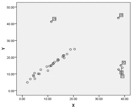
A scatter plot for the data is shown in Figure 1.

From Figure 1, the majority of the observations follow a linear pattern. Five observations {28, 29, 30, 31, 32} lie separately from the bulk of the data. These observations are suspected to be outliers. Observation 28 is outlying with respect to its x value. This observation is not influential because, it lies along the pattern of the bulk of the data. It can be seen from Figure 1 that observation 29 is outlying with respect to its y value, and therefore may be influential. Further, observations {30, 31, 32} are outliers with respect to their x and y values. These observations are also influential.

A simple regression analysis of the artificial data yields a regression model summary which is presented in Table 1.

Table 1. Regression Model Summary for Artificial Data

Model R sq Adj. R sq Std Error of Estimate

1 0.203 0.177 7.647

From Table 1, it is observed that as low as 20.3% of the variation in the response Variable Y is accounted for by the predictor variable X.

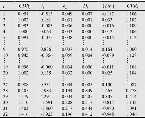
We now examine the performances of the measures of influence for this dataset. The results are shown in Table 2. From Table 2, the CDRi measure detects observations {28, 29, 30, 31, 32} as outliers (by means of an index plot, in Appendix A, of the values of CDR_i). These observations have CDR_i values that markedly deviate from unity. Also, each of D_i and (DFFITS)i detected observations {28, 29,

30, 31, 32} as outliers. The values of D_i exceed

the cut-off value if 0.133

2 32

4 ) 1 (

4

= − = + − ≥

k n

Di . Also,

these observations have absolute values of (DFFITS)i that

exceed the calibration point of 0.5.

The t_i measure suggests that observations 28 and 29 are outliers since their absolute ti values exceed the cutoff point t_0.05,29=±2.045. In addition, h_ii identifies observations 28, 30, 31, and 32 to be outlying but not 29. Their values are greater than twice the average of all leverage values (0.125). Finally, it can be seen that the

i

CDR , just like t_i, classifies only observations 28 and 29 as suspect outliers. The values of CDR_i for observations 28 and 29 do not fall within the cutoff interval (0.813, 1.188). It is worth noting that the CDRi, besides Di and

, )

(DFFITS _i is successful in detecting all the outliers in the data. However, hii identifies all but one outlier. Each of ti and CDR_i detect only two of the five outliers.

Next, we consider an assessment of the influence of the outlying sets of observations on the value of R2. The results are presented in Table 3. The table gives the change

in 2

R when the specified observations have been deleted from the data for each of the measures.

Table 2. Influence Measures for Artificial Data

i CDRi ti hii Di (DF)i CVRi 1 0.951 -0.513 0.049 0.007 -0.117 1.106 2 1.002 0.181 0.031 0.001 0.033 1.102 3 0.993 -0.083 0.036 0.000 -0.016 1.109 4 1.000 0.063 0.033 0.000 0.012 1.106 5 0.991 -0.075 0.038 0.000 -0.015 1.112

⋮ ⋮ ⋮ ⋮ ⋮ ⋮ ⋮

9 0.975 0.836 0.037 0.014 0.164 1.060 10 0.945 -0.356 0.059 0.004 -0.089 1.128

⋮ ⋮ ⋮ ⋮ ⋮ ⋮ ⋮

19 0.996 -0.060 0.034 0.000 -0.011 1.108 20 1.002 0.135 0.032 0.000 0.025 1.104

⋮ ⋮ ⋮ ⋮ ⋮ ⋮ ⋮

27 0.988 0.531 0.034 0.005 0.100 1.087 28 0.405 2.983 0.194 0.849 1.465 0.778 29 1.579 4.291 0.034 0.205 0.805 0.414 30 1.310 -1.591 0.208 0.317 -0.817 1.143 31 1.403 -1.860 0.217 0.444 -0.980 1.091 32 1.416 -1.923 0.196 0.412 -0.948 1.046

Table 3. Effect of Deletion of Outlying Observations on R2Value

Measure Outlying Observations

2 new

R 2

R change

i

t 28, 29 0.185 -0.018

ii

h 28, 30, 31, 32 0.546 0.343

i

CVR 28, 29 0.185 -0.018

i

D 28, 29, 30, 31, 32 0.975 0.772 i

DF _{28, 29, 30, 31, 32 0.975 0.772} i

CDR 28, 29, 30, 31, 32 0.975 0.772

Table 3 indicates that the omission of the observations {28, 29, 30, 31, 32} from the dataset results in an increase in the value of 2

R from 0.203 to 0.975, a substantial increase using the CDR. The result is the same for Di and

, )

(DFFITS _i denoted DFi in the table.

3.2. Using CDR to Detect Outliers in Multiple Linear Regression Analysis

For illustrative purposes, we use the data by Moore [9] (as cited in [10]). This data has also been used by [9] to compare the performance of various influence measures to detect influential observations, high leverage points, and outliers in linear regression. The measured variables are:

Y― log (oxygen demand in dairy waste), mg/min;

1

X ― biological oxygen demand, mg/litre;

2

X ― total Kjeldahl nitrogen, mg/litre;

3

X ― total solids, mg/litre;

4

X ―total volative solids (a component of X3), mg/litre;

5

X ―chemical oxygen demand, mg/litre.

Correlation analysis of the data shows the presence of some linear relationship between Y and each of the predictor variables, except X2. Further, there is somewhat strong positive linear relationship between any pair of the variables

1

X , X3, X4, and X5. These linear associations among the predictor variables are likely to pose multi-collinearity problems. The summary of the fitted regression of Y _{on the}

Table 4. Regression Model Summary for Moore’s Data

Model R sq Adj. R sq Std Error of Estimate

Full 0.811 0.743 0.262

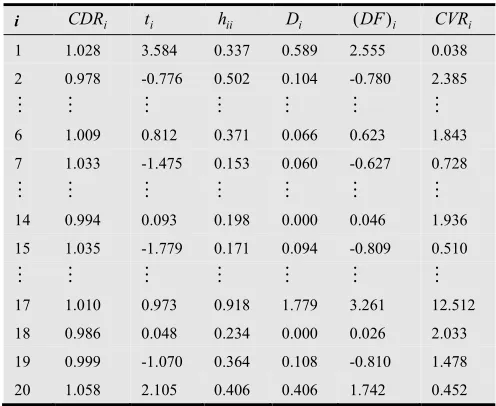
Table 5. Influence Measures for Moore’s Data

i CDRi ti hii Di (DF)i CVRi 1 1.028 3.584 0.337 0.589 2.555 0.038 2 0.978 -0.776 0.502 0.104 -0.780 2.385

⋮ ⋮ ⋮ ⋮ ⋮ ⋮ ⋮

6 1.009 0.812 0.371 0.066 0.623 1.843 7 1.033 -1.475 0.153 0.060 -0.627 0.728

⋮ ⋮ ⋮ ⋮ ⋮ ⋮ ⋮

14 0.994 0.093 0.198 0.000 0.046 1.936 15 1.035 -1.779 0.171 0.094 -0.809 0.510

⋮ ⋮ ⋮ ⋮ ⋮ ⋮ ⋮

17 1.010 0.973 0.918 1.779 3.261 12.512 18 0.986 0.048 0.234 0.000 0.026 2.033 19 0.999 -1.070 0.364 0.108 -0.810 1.478 20 1.058 2.105 0.406 0.406 1.742 0.452

From Table 4, we note that even though the _R2 _{value is} high, it may not be a true representation of the explanatory power of the fitted regression model. In an ideal situation, each observation in the dataset contributes equally to the formation of the value of 2

R . It is, therefore, legitimate to assess each observation vis-à-vis their influence on

2

R value in order to identify unusual ones.

Table 5 shows the values of various measures of influence for Moore’s data when the ith observation is omitted from the dataset.

First, we consider the coefficient of determination ratio (CDR) in Table 5. It can be observed that the (CDR) for all observations are approximately equal to one except observations {1, 7, 15, 20}. The removal of these observations from the dataset is expected to substantially

improve the 2

R . Therefore, the observations {1, 7, 15, 20} are influential.

To evaluate the studentised deleted residual ti for an

observation, we compare this quantity with

2

α

t based on

) 2

(n−k− degrees of freedom. Specifically, if the t_i is greater in absolute value than

2 ,

2 n−k−

t_α , then there is some evidence that the observation is an outlier with respect to its

y value. From Table 5, we see that the ti for observations 1 and 20 (3.584 and 2.105, respectively) are both greater than

. 771 . 1

13 , 05 .

0 =

t Therefore, we should be very concerned that

{1, 20} are outliers with respect to their y values.

For the Moore’s data, there are n=20 observations and since the fitted linear regression model utilizes

5 =

k independent variables, twice the average leverage value is 0.60.

From Table 5, we see that the leverage value for observation 17 is 0.9182. Since this value is greater than 0.60, it suggests that observation 17 is an outlier with respect to its x values.

From Table 5, Cook’s distance for each of observations {1, 17, 20} is greater than the cut-off value 0.267. This means that removing the group of observations {1, 17, 20} from the dataset would substantially change the least squares estimate of the regression parameters. Hence, observations 1, 17, and 20 are flagged as influential.

It can be seen in Table 5 that the DFFITS for observations 1, 17, and 20 exceed the cut-off value of 1.095, and therefore, they should be identified as outliers.

For the Moore’s data, the cutoff values for CVRi is

) 900 . 1 , 100 . 0

( . The cut-off interval is rather conservative in

that it declares too many observations as outliers. In view of this, we use the index plot (see Appendix B) of CVRi to find

outliers. Observations 1 and 17 are considered as outliers. The CVRi value for observation 17 is the largest indicating

that its presence would have the greatest impact on increasing the precision of the parameter estimates. The

i

CVR for observation 1 is the lowest. This shows that the presence of observation 1 in the dataset greatly decrease the precision of the estimates.

The influence of the different sets of suspect outlying observations, from the various measures of influence, on the

value of 2

R is displayed in Table 6.

Table 6. Effect of Deletion of Outlying Observations on R2Value

Measure Outlying Observations

2 new

R 2

R change

i

t 1, 20 0.895 0.084

ii

h 17 0.819 0.008

i

CVR 1, 17 0.832 0.021

i

D 1, 17, 20 0.893 0.082

i

DF 1, 17, 20 0.893 0.082

i

CDR 1, 7, 15, 20 0.938 0.127

It is observed from Table 6 that the 2

R value has increased as a result of deleting various sets of suspect outlying observations. However, the magnitude of the increment differs across the sets of outlying observations. The greatest change in 2

R value (from 0.811 to 0.938) is associated with the omission of the outlying set {1, 7, 15, 20}, which is based on the CDR_i measure of influence. However, the least change in 2

R value is linked with the omission of {17}, which is based on the h_ii measure of influence. A comparison of values of _R2 _{in Table 6 shows} that the set of observations {1, 7, 15, 20} detected by CDR_i

is the most influential than those emanating from the other measures of influence. The deletion of this set from the dataset would subsequently lead to a substantial change in the regression estimates. The result shows that the CDRi is

4. Conclusion and Recommendation

The main objective of the paper was to assess the standard measures for detecting influential outliers in structured data. The result shows that the new measure, called the Coefficient of Determination Ratio (CDR_i) identifies suspect outliers which all the other measures detect. In addition, it has the property to detect other and even more subtle suspect outlier observations which other measures do not detect. This means that by using the CDR_i , any observation which is potentially an outliers can be identified for assessment. The benefit of using this method is that the significance of the model obtained eventually for summarising the dataset is more reliable.

The results also show that the CDR, Di , and DFi

detect almost the same sets of influential outliers. However, the CDR always perform distinctly from the other influence measures such as the t_i, hii, and CVRi.

The implementation of the new method relied mostly on the scatter plot of the values of the CDR. Like the other measures, it would be more formal to identify suspect outliers using exact cut-off values. Future studies in this area should focus on obtaining a generalized cut-off value for the new measure.

Appendix A

Index Plots for Artificial Data

(a) (b)

(c) (d)

(e) (f)

Appendix B

Index Plots for Moore’s Data

(a) (b)

(c) (d)

(e) (f)

Appendix C

Proof of Coefficient of Determination Ratio

The CDR for the ith observation is defined as

2 2 ) (

R R

CDR_i= i , i=1,2,⋯,n ₍₁₎

or

SSR SSR SST

SST

CDR i

i i

) (

) (

×

= (2)

Now SSR(i)=βˆ(′i)X′(i)X(i)βˆ(i). It can be shown ([7]) that

,

) ( ) ( )

(i i i i i

( )

i ii

i i

h XX x

β

β₍₎ 1

1 ˆ ˆ

ˆ _′ −

− − =

′ ε . (3)

Substituting yˆ=Xβˆ, we have

y y β X X β ′ ′ ′

=ˆ ˆ

2 R and ) ( ) ( ) ( ) ( ) ( ) ( 2 ) ( ˆ ˆ i i i i i i i R y y β X X β ′ ′ ′

= . Substituting, we have

) ( ) ( ) ( ) ( ) ( ) ( ) ( ) ( )

(i i i ˆi( i i)ˆi ˆi ˆi ˆi i iˆi

SSR =X′ X =β′ X′X−xx′ β =β′ X′Xβ −β′ xx′β

Further substitutions using Eq. (3) gives

( )

( )

( )

( )

( )

( )

( )

( )

      ′ ′ − − ′       ′ ′ − − ′ −       ′ − − ′       ′ − − =       ′ − − ′′ ′       ′ − − −       ′ − − ′ ′       ′ − − = − − − − − − − − i i ii i i i i i ii i i i ii i i ii i i ii i i i i ii i i ii i i ii i i h h h h h h h h SSR x X X x 1 ˆ βˆ x x X X x 1 ˆ βˆ x x X X X 1 ˆ βˆ X x X X X 1 ˆ βˆ X x X X 1 ˆ βˆ x x x X X 1 ˆ βˆ x X X 1 ˆ βˆ X X x X X 1 ˆ βˆ 1 1 1 1 1 1 1 1 ) ( ε ε ε ε ε ε ε ε

Substituting x_i′βˆ=yˆ_i and h_ii=x′_i

( )

X′X−1x′_i we have

( )

( )

      − −       − − −       ′ − −       ′ ′ ′ − − ′ ′ = − − ii ii i i ii ii i i i ii i i ii i i h h y h h y h h SSR 1 ˆ ˆ 1 ˆ ˆ x X X X 1 ˆ βˆ X X X X x 1 ˆ X

βˆ 1 1

) ( ε ε ε ε Expanding gives

( )

( ) ( )

( ) ( )( )

2 2 2 1 1 2 1 1 ) ( 1 ˆ ˆ 1 ˆ βˆ x 1 ˆ x βˆ 1 ˆ βˆ X X βˆ 1 ˆ ˆ x X X X X X X x 1 ˆ βˆ X X X X x 1 ˆ x X X ) X X ( βˆ 1 ˆ βˆ X X βˆ         − − −         − + ′ − − ′ − − ′ ′ =         − − − ′ ′ ′ ′         − + ′ ′ ′ − − ′ ′ ′ − − ′ ′ = − − − − ii ii i i ii ii i i ii i i ii i ii ii i i i i ii i i ii i i ii i i h h y h h h h h h y h h h SSR ε ε ε ε ε ε ε ε

Substitution for yˆ_i=y_i−εˆ_i, further simplification gives

(

)

(

)

2

2

( ) 2

2 2

2

2 2

ˆ ˆ ˆ

2 ( )

ˆ ˆ _{( ˆ)}

1 1

ˆ 2 (ˆ ˆ)

1 1

ˆ 1

i i i i ii

i i i

ii ii

i ii i i i ii

ii ii i i ii y h SSR y h h

h y h

h h

SSR y h

ε ε ε _ε

ε ε ε

ε − ′ ′ = − + − − − − − − + − − = − + − β X Xβ

(4)

Now,

2 )

(i SST yi

SST = − . (5)

Substituting Eq (4) and (5) into Eq (2) yields

SSR h y SSR y SST SST CDR ii i i i

i _

      − + − − = 1 ˆ2 2 2 ε

Some few further steps gives

        − − − − − = ii i i i i i h y y SST R SST y CDR 1 ˆ ) ( 1 1

1 ₂ 2

2 2 2 ε .

References

[1] Barnett, V., & Lewis, T. (1994). Outliers in statistical data (3rd ed.). New York, NY: John Wiley and Sons.

[2] Cohen, J., Cohen, P., West, S. G., & Aiken, L. S. (2003). Applied multiple regression/correlation analysis for the behavioral sciences (3rd ed.). London, England: Lawrence Erlbaum Associates.

[3] Weisberg, S. (2005). Applied linear regression (3rd ed.). New York, NY: John Wiley and Sons.

[4] Nurunnabi, A. A. M., Imon, A. H. M. R., Ali, A. B. M. S., & Nasser, M. (2011). Outlier detection in linear regression.

Retrieved June 9, 2011 from

http://irma-international.org/chapter/outlier-detection-linear-regression/53318/

[5] Chatterjee, S., & Hadi, A. S. (1988). Sensitivity analysis in linear regression. New York, NY: John Wiley & Sons.

[6] Cook, R. D. & Weisberg, S. (1982). Residuals and Influence in Regression. New York, NY: Chapman and Hall.

[7] Rencher, A. C. & Schaalje, G. B. (2008). Linear models in statistics (2nd ed.). New Jersey, NJ: John Wiley & Sons.

[8] Siniksaran, E. & Satman, M. H. (2011). PURO: A package for unmasking regression outliers. Gazi University Journal of Science, 24 (1), 59-68.

[9] Moore, J. (1975): Total biochemical oxygen demand of dairy manures. Ph. D. Thesis, Univ. of Minnesota, Dept. Agricultural Engineering.