Comparative Study on Forecasting Accuracy among Moving Average Models with Simulation and PALTEL Stock Market Data in Palestine

Published online November 10, 2013 (http://www.sciencepublishinggroup.com/j/ajtas) doi: 10.11648/j.ajtas.20130206.17

Comparative study on forecasting accuracy among

moving average models with simulation and PALTEL

stock market data in Palestine

Samir K. Safi

1

, Issam A. Dawoud

2

1

Dept. of Economics and Statistics, Faculty of Commerce, The Islamic University of Gaza, Gaza, Palestine 2

Dept. of Statistics, The Faculty of Science, Çukurova University, Adana, Turkey

Email address:

[email protected](S. K. Safi), [email protected](I. A. Dawoud)

To cite this article:

Samir K. Safi, Issam A. Dawoud. Comparative Study on Forecasting Accuracy among Moving Average Models with Simulation and PALTEL Stock Market Data in Palestine. International Journal of Theoretical and Applied Statistics. Vol. 2, No. 6, 2013, pp. 202-209. doi: 10.11648/j.ajtas.20130206.17

Abstract:

In this paper, we discuss three analytical time series models for selecting the more effective with an accurate forecasting models, among others. We analytically modify the stochastic realization utilizing (i) k-th moving average, (ii)

k-th weighted moving average, and (iii) k-th exponential weighted moving average processes. The examining methods have been applied for 1000 independent datasets for five different parameters with possible orders p q+ ≤5. We consider stationary data

(

d =0

)

, and non-stationary data with first and second differences

(

d=1, 2

)

for ARIMA models. We consider short term

(

n=50

)

and long term,

(

n=500

)

observations. A similar forecasting models was developed and evaluated for the daily closing price of Stock Price of the PALTEL company in Palestine. The main finding is that, in most simulated datasets one or more of the proposed models give better forecast accuracy than the classical model (ARIMA). Specially, in most simulated datasets 3– time Exponential Weighted Moving Average based on Autoregressive Integrated Moving Average (EWMA3-ARIMA) is the best forecasting model among all other models. For PALTEL Stock Price, the best forecasting model is 3–time Moving Average based on Autoregressive Integrated Moving Average (MA3-ARIMA) among all other models.

Keywords:

Moving Average, Weighted Moving Average, Exponential Weighted Moving Average, Stationary, Forecasting Accuracy, ARIMA Models

1. Introduction

In this section, we introduce some literature review that have been developed recently. Trigg and Leach [15] initiated a study of automatically monitoring a forecasting process to assure that the forecast remains in control. They utilized a first order exponential model with data that contained jumps.

Crane and Eeatly [6] applied the exponential process forecasts along with other independent variables into developing a multiple regression model. This combined forecasting procedure was applied in modeling some economic data series related to bank deposits.

Shami and Snyder [11] focused on the relationship between the exponential smoothing methods of forecasting and the integrated autoregressive moving average models

underlying them. They derived the general linear relationship between their parameters. They proposed to determine the pertinent quantities in this relation. This study was illustrated on common forms of exponential smoothing and also applied to a new seasonal form of exponential smoothing with seasonal indexes which always sum to zero.

maximum likelihood methods are used in conjunction with exponential smoothing to estimate the smoothing parameters. The results indicated that the information criterion approach appears to provide the best basis for an automated approach to method selection, provided that it is based on A kaike’s information criterion.

Parthasarath and Levinson [10] studied the evaluating the accuracy of demand forecasters using a sample of recently completed projects in Minnesota and identified the factors influencing the inaccuracy in forecasts. The analysis indicated a general trend of underestimation in roadway traffic forecasts with factors. The comparison of demographic forecasts showed a trend of overestimation while the comparison of travel behavior characteristics indicates a lack of incorporation of fundamental shifts and societal changes.

Steiner [14] showed proposed a version of exponentially weighted moving average (EWMA) control charts applicable to monitoring the grouped data for process shifts. The runs length properties of this new grouped EWMA charts are compared with similar results previously obtained for EWMA charts variables data with those for Cumulative Sum (CUSUM) schemes based on grouped data. Grouped data EWMA charts are shown to be nearly as efficient as variables based EWMA charts, and are thus an attractive alternative when collection of variables data is not feasible. In addition, grouped data EWMA charts are less affected by the inherent in grouped data than are grouped data CUSUM charts.

Shih and Tsokos [12] showed a new time series that is based on the actual stochastic realization of a given phenomenon. The proposed model is based on modifying the given economic time series, {x_t}, and smoothing it with k-time moving average to create a new time series, {y_t} . The basic analytical procedure are developed through the developing process of a forecasting model. A step by step procedure is mentioned for the final computational procedure for a non stationary time series. They evaluated the effectiveness of their proposed models by selecting a company from the Fortune (500) list, company XYZ the daily closing prices of the stock for 500 days was used as their time series, {x_t}, which was as usual non-stationary. They developed the classical time series forecasting model using Box and Jenkins methodology and also their proposed model, {y_t}, based on a 3-way moving average smoothing procedure. The analytical form of the two forecasting models is presented and a comparison of them is also given. Based on the average mean residual, the proposed model was significantly more effective in such terms of predicting of the closing daily prices of the stock XYZ.

Tsokos [16] investigated the effectiveness of developing a forecasting model of a given non stationary economic realization using a k-th moving average, a k-th weighted moving average and a k-th exponential weighted moving average process. They created a new non-stationary time series from the original realization using the three different

weighted methods. Using real economic data, they formulated the best ARIMA model and compare short term forecasting results of the three proposed models with that of the classical ARIMA model. In all cases the new models give better short term forecasting results than classical ARIMA model.

Some times method of Box and Jenkins may be not optimal for giving a forecasting model for the actual data. For this reason, proposed technique has been developed by modifying a new k-time moving average time series in three proposed models (a k-th moving average, a k-th

weighted moving average and a k-th exponential weighted moving average), In this paper, we compare these proposed models for forecasting accuracy with the classical ARIMA model by using simulation and real data set, namely daily closing price of Stock Price of the PALTEL company in Palestine.

This paper is organized as follows: Sections 2 presents some fundamental definitions; Sections 3 displays the measures of forecasting accuracy; section 4 demonstrates the simulation study; results for PALTEL stock market data is shown in section 5; and Section 6 summarizes the important results and offers suggestions for future research.

2. Fundamental Definitions

In this section, we show some fundamental concepts that are essential for dealing with time series models. We introduce autoregressive integrated moving average model, ARIMA(p,d,q) and three additional models, namely the k

-th Simple Moving Average (SMA), the k-th Weighted Moving Average (WMA), and the k-th Exponential Weighted Moving Average (EWMA).

2.1. Definition 1. (ARIMA model)

The classical A RIMA p d q( , , ) autoregressive integrated moving average is defined as

( )(

1

)

d

( )

p B B xt q B t

ϕ − =θ ε (2.1)

where, B xj _t =x_t−j , (1−B)d is the difference filter, d

is the degree of differencing of the series,

( )

(

2

)

1 2

1 p

p B B B pB

ϕ = −ϕ −ϕ − ⋯−ϕ , and

( )

(

2

)

1 2

1 q

q B B B qB

θ = −θ −θ −⋯−θ .

2.2. Definition 2. (The K-th SMA Process )

The k-th SMA process of a time series {x_t} is given by

1

1 0

1k

t t k j

j

y x

k

−

− + + =

=

∑

(2.2)

where,

t

=

k

,

k

+

1

,

…

,

n

.

observations of {y_t} decreases, and the series {y_t} gets closer and closer to the mean of the series{x_t}. In addition, when k =n , the series {y_t} reduces to a single observation, and equals to

µ

, because

1 n j j t x y n µ = = =

∑

_(2.3)

In time series analysis, the primary use for the k-th SMA is for smoothing a time series and it is very useful in discovering short – term, long – term trends and seasonal components of a time series.

2.3. Definition 3. (The SMA Back-Shift)

Using the model that we developed for {y_t} in Definition (2) and subject to the Akaike’s information criterion (AIC) criteria, we forecast values of {y_t} and proceed to apply the back–shift operator to obtain estimates of the original phenomenon {x_t}, that is,

1 2 1

ˆ_t ˆ_{t t t t k}

x =k y −x₋ −x₋ − ⋯−x_{− +} (2.4)

2.4. Definition 4. (The WMA Process)

The k-th WMA process of a time series {x_t} is defined as:

(

)

1 1 0 ( 1) 1 2 k

t k j

j t j x z k k − − + + = + = +

∑

(2.5)

where, t =k k, +1,…,n.

Similar to the moving average process, as k increases, the number of observations of the series{ }z_t decreases, and as k →n , from (2.2) the series { }z_t becomes

(

1 1

)

2

n j j t j x z n n = = +

∑

(2.6)

The k-th WMA process puts more weight on the most recent observation, and the weight consistently decreases up to the first observation. In addition, it captures the original time series better than the SMA process, which is suitable for those analysts who believe the recent observations should weight more than the old ones.

2.5. Definition 5. (The WMA Back-Shift)

Using the model that we developed for { }z_t in Definition (4) and subject to the AIC criteria, we forecast values of { }z_t and proceed to apply the back–shift operator to obtain estimates of the original phenomenon {x_t}, that is

1

2

1

ˆ

[(1 ) /2]

( 1)

(

2)

ˆ

_t

k k

z

t

k

x

t

k

x

t

x

t k

x

k

−

−

− +

+

− −

− −

− −

=

⋯

(2.7)

2.6. Definition 6. (The EWMA Process)

The k-th EWMA process of a time series{x_t}is defined as follows: 1 1 1 0 1 0

(1

)

(1

)

k k j

t k j j t _k j j

x

α

ν

α

− − − − + + = − =

−

=

−

∑

∑

(2.8)

where, t =k k, +1,…,n

, and the smoothing factor

α

is

defined as 2 1 k α= + _.

As k increases, the number of observations the series { }v_t

decreases, and it eventually reduces to a single observation when k =n . As k →n , the series { }vt

becomes 1 1 1 0 1 0 (1 ) (1 ) n n j j j t _n j j x α ν α − − − + = − = − = −

∑

∑

(2.9)

Equation (2.9) shows that the exponential weighted moving average process weighs heavily on the most recent observation and decreases the weight exponentially as time decreases.

2.7. Definition 7. (The EWMA Back-Shift)

Using the model that we developed for { }v_t in Definition (6) and subject to the AIC criteria, we forecast values of

{ }v_t and proceed to apply the back – shift operator to obtain estimates of the original phenomenon {x_t}, that is,

2 1

1 2 1

1

0

ˆ

ˆ

(1

)

(1

)

(1

)

(1

)

k t

t k t t t k

j

j

x

ν

α

x

α

x

α

x

α

−

− − − −

−

=

=

− −

− −

− − −

−

∑

⋯

(2.10)

3. Measures of Forecasting Accuracy

Many measures of forecasting accuracy have been developed, and several authors have been discussed the fundamentals usage for these measurements and made comparisons among the accuracy of forecasting methods in univariate time series data, see for example Brockwell and Davis [5], Cryer and Chan [7], Harvey [8], Hyndman and Koehler [9], Shumway and Stoffer [13], Wei [17], among others.

3.1. Scale – Dependent Measures

There are some commonly used accuracy measures whose scale depends on the scale of the data. These measures are useful for comparing different models on the same set of data. The most commonly used scale – dependent measures are based on the absolute error or squared errors. For example

2

t

t

t

Mean Square Error (MSE) = mean (e )

Root Mean Square Error (RMSE) = MSE

Mean Absolute Error (MAE) = mean ( |e | )

Median Absolute Error (MDAE) = median (|e | )















(3.1)

where, e_t =x_t −F_t is the forecast error, x_t the observations at time t , F_t the forecast of x_t. Historically, the RMSE and MSE have been popular, largely because of their theoretical relevance in statistical modeling, Hyndman and Koehler [9]. However these measures are more sensitive to outliers than MAE or MDAE which has led some authors, for example, see Armstrong [1] to recommend using other forecast accuracy measures.

3.2. Measures Based on Percentage Errors

Percentage errors have the advantage of being scale – independent, and so are frequently used to compare forecast performance across different data sets. The most commonly used measures:

t t 2 t

Mean Absolute Percenatge Error (MAPE) = mean (|p | )

Median Absolute Percentage Error (MdAPE) = median(|p | )

Root Mean Square Percentage Error (RMSPE) = mean( p )

Root Median Square Percentage Error (RMdSPE) = media

n( p )

2_t















(3.2)

where, the percentage error is given by _t 100 t

t

e p

x

= ,

t t t

e =x −F , x_t the observations at time t , F_t the forecast of x_t.

These measures have the disadvantages of being infinite or undefined if x_t =0 for any

t

in the period of interest, and having an extremely skewed distribution when any x_t

is close to zero, Hyndman and Koehler [9].

3.3. Measures Based on Relative Errors

An alternative way of scaling is to divide each error by the error obtained using another standard method forecasting. The relative error is defined as follows:

*

t

t

t

e

r

e

=

(3. 3)

benchmark method. Then we can define:

t

t

t

Mean Relative Absolute Error (MRAE) = mean ( |r | )

Median Relative Absolute Error (MdRAE) = median (|r |)

Geometric Mean Relative Absolute Error (GMRAE) = gmean (|r |)











(3.4)

Armstrong, J., and Collopy, F. [2] recommended the GMRAE when the task involves calibrating a model for a set of time series. The GMRAE compares the absolute error of a given method to that from the random walk forecast. For selecting the most accurate methods, they recommended the MdRAE when few series are available.

3.4. Relative Measures

Rather than use relative errors, one can use relative measures. By letting MAEb denote the MAE from the

benchmark method, then the relative

MAE

is given by

b

MAE RELMA E

MA E

= (3.5)

An advantage of this method is their interpretability. i.e., the relative MA E measures the improvement possible. From the proposed forecast method relative to the benchmark forecast method. A ratio less than one indicates that the proposed method is more efficient than the benchmark method and if the ratio is close to one, then the proposed method is nearly as efficient as the benchmark method.

4. Simulation Study

In this section, we consider the robustness of various time series models, including the estimated k−th moving average and ARIMA models. These simulations examine the usefulness and effectiveness for the proposed model. In particular, how do the estimated k−th moving average models perform relative to the classical ARIMA model? We compare the finite sample efficiencies of ARIMA models relative to three k−th moving average models: the k−th

simple moving average; k−th weighted moving average; and k-th exponential weighted moving average processes.

Starting with a non-stationary time series of a short term and long term simulated data such that we applied 1000 simulated data sets of each parameter for Autoregressive Moving Average models such that each data set of short term contains 50 observations and long term contains 500 observations. we analytically use a k−th moving average, a

k−th weighted moving average and k−th exponential

moving average. A residual analysis based on the criteria of a forecast accuracy comparison of these forecasting models is given. R-statistical software is used for fitting the different time series models.

4.1. The Simulation Setup

Two finite sample sizes, short term with size N=50, and long term with size N=500 are used. In addition, four non-stationary time series models are used; classical ARIMA;

k−th moving average, a k−th weighted moving average; and

k−th exponential moving average. We also generated a time series for each model of length 1000 for different orders of

p and q with all possibilities p q+ ≤5 with stationarity data (d =0), and nonstationarity data with first and second differences (d =1, 2).

We generate the four non-stationary time series models and select the most appropriate models with the smallest AIC and the smallest average mean square error. In addition, Shih and Tsokos [12] summarized the development of the model as follows:

• Transforming the original times series {x_t} into

t t t

{y , z , v } by using equations (2.2), (2.5), and (2.8), respectively.

• Check for stationary of time series by determining the order of differencing d , where d =0,1, 2,… according to KPSS test, Box et al. [4] until we achieve stationarity.

• Deciding the order

m

of the process, where

m = +p q.

• After ( ,d m) being selected, listing all possible set of ( , )p q for p q+ ≤m.

• For each set of ( , )p q , estimating the parameters of each model, that is,

ϕ ϕ

₁, ₂,…,

ϕ θ θ

_p, ₁, ₂,…,

θ

_q. • Compute the AIC for each model, and choose the

one with smallest AIC.

• Solve the estimates of the original time series by using equations (2.4), (2.7), and (2.10), respectively.

4.2. The Simulated Selected Models

Table 4.1. The Simulated Selected Models

Models The Simulated Models

Short term (N=50)

ARIMA:A RIMA(1,1,1) xt=1.91xt−1−0.91xt−2+ +εt 0.10εt−1

SMA: A RIMA(2 ,1, 2) yt=2.40yt−1−1.84yt−2+0.45yt−3+εt+1.37εt−1+0.42εt−2

WMA:A RIMA(1,1, 2) zt=1.94zt−1−0.94zt−2+ +εt 1.63εt−1+0.67εt−2

EWMA:A RIMA(1,1, 2) νt=1.93νt−1−0.93νt−2+ +εt 1.56εt−1+0.56εt−2

Long term (N=500)

ARIMA: A RIMA(1,1,1) xt =1.92xt−1−0.92xt−2+ +εt 0.92εt−1

SMA: A RIMA(1,1, 4) yt=1.92yt 1− −0.92yt 2− + ε +t 1.92εt 1− +1.92εt 2− +0.91εt 3− +0.001εt 4−

WMA:A RIMA(1,1, 3) zt=1.91zt−1−0.91zt−2+εt+1.60εt−1+0.10εt−2+0.34εt−3 EWMA:A RIMA(1,1, 3) νt=1.91νt−1−0.91νt−2+ +εt 1.43εt−1+0.75εt−2+0.26εt−3

4.3. The Simulation Results

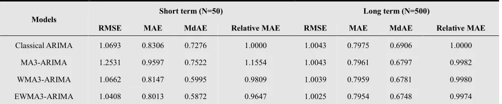
Table (4.2) shows the comparison between the proposed models versus classical models for short and long terms based on selected criterion of forecasting accuracy for simulated models. The results show that the EWMA3-ARIMA model is preferable in selecting the most appropriate forecasting model over all the other models for short and long terms. In addition, the WMA3-ARIMA model performs better than the classical ARIMA model.

Furthermore, the relative

MAE

measures for EWMA3-ARIMA to the classical EWMA3-ARIMA equal 0.9647. This result indicates that EWMA3-ARIMA model is more efficient than the other models for long and short terms. In addition, the WMA3-ARIMA model is more efficient than the classical ARIMA model based on relative MAE measures the Classical ARIMA model. The other measures of forecasting accuracy criterion mimic similar results.

Table 4.2. Criterion of Forecasting Accuracyfor Simulated Models

Models

Short term (N=50) Long term (N=500)

RMSE MAE MdAE Relative MAE RMSE MAE MdAE Relative MAE

Classical ARIMA 1.0693 0.8306 0.7276 1.0000 1.0043 0.7975 0.6906 1.0000

MA3-ARIMA 1.2531 0.9597 0.7522 1.1554 1.0043 0.7961 0.6797 0.9982

WMA3-ARIMA 1.0662 0.8147 0.5995 0.9809 1.0039 0.7959 0.6781 0.9980

EWMA3-ARIMA 1.0408 0.8013 0.5872 0.9647 1.0025 0.7954 0.6748 0.9974

Therefore, 3 – time Exponential Weighted Moving Average based on Autoregressive Moving Average (EWMA3-ARIMA) outperforms and preferable in selecting the most appropriate forecasting model over all the other models for short and long terms. This result of both short and long terms reveals that EWMA3-ARIMA outperform and offer consistent forecasting performance compared to ARIMA model and hence preferable as a robust forecasting model for simulated data.

5. Illustrative Example: PALTEL Stock

Market Data

Table 5.1. Selected Models for PALTEL Stock Market Data

Models The Simulated Models

ARIMA: A RIMA(5 ,1, 3) 1 2 3 4 5 6

1 2 3

1.532 1.291 0.422 0.424 0.1982 0.110

0.341 0.672 0.376

t t t t t t t

t t t t

x x x x x x x

ε ε−− −ε− −ε− − − −

− + − − + −

= − + +

SMA: A RIMA(5 ,1, 5) 1 2 3 4 5 6

1 2 3 4 5

2.069 1.783 0.389 0.486 0.252 0.092 0.124 0.638 0.011 0.864 0.355

t t t t t t t t t t t t t

y y y y y y y

ε ε−− ε−− ε−− ε−− ε−− −

− + − − + −

= + + − + +

WMA:A RIMA(6 ,1, 3) 1 2 3 4 5 6 7

1 2 3

2.175 2.374 1.270 0.349 0.804 0.534 0.150

0.322 0.660 0.390

t t t t t t t t

t t t t

z z z z z z z z

ε ε ε ε

− − − − − − −

− − −

− + − − + − +

= − + +

EWMA:A RIMA(2 ,1, 6) 1 2 3 1 2

3 4 5 6

1.771 1.707 0.936 0.078 0.767

0.322 0.297 0.053 0.045

t t t t t t t

t t t t

ν ν ν ν ε ε ε

ε ε ε ε

− − − − −

− − − −

− + − = − +

+ + − −

5.1. Selected Models for PALTEL Stock Market Data Table (5.1) shows the selected real time series models based on the criterion that we have mentioned in section 3

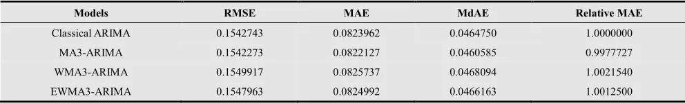
5.2. Criterion of Forecasting Accuracy

Table (5.2) shows the comparison between the proposed

models versus classical models for PALTEL stock market data based on selected criterion of forecasting accuracy. The results show that the MA3-ARIMA model outperforms in selecting the most appropriate forecasting model over all the other models for PALTEL data. The other measures of forecasting accuracy criterion mimic similar results.

Table 5.2. Criterion of Forecasting Accuracyfor Real Data models

Models RMSE MAE MdAE Relative MAE

Classical ARIMA 0.1542743 0.0823962 0.0464750 1.0000000

MA3-ARIMA 0.1542273 0.0822127 0.0460585 0.9977727

WMA3-ARIMA 0.1549917 0.0825737 0.0468094 1.0021540

EWMA3-ARIMA 0.1547963 0.0824992 0.0466163 1.0012500

6. Conclusion and Future Research

In this paper, we have examine the sensitivity of model selection based on criterion of forecasting accuracy for the classical ARIMA model and three proposed models, k-th

moving average, k-th weighted moving average, and k-th

exponential weighted moving average models. The main finding of the simulation result is that 3–days Exponential Weighted Moving Average based on Autoregressive Moving Average (EWMA3-ARIMA) is preferable, and outperforms, and more efficient than the classical ARIMA model for long and short terms data. In addition, for PALTEL stock market data, the 3–days Moving Average based on Autoregressive Moving Average (MA3-ARIMA) model outperforms in selecting the most appropriate forecasting model over all the other models.

Many opportunities of future research are available. Determine the optimal value of k that will produce the smallest residuals and the best forecasting model based on criterion of forecasting accuracy. Examine the robustness and sensitivity of the proposed models when k changes. In addition, construct the confidence limits for short and long terms forecasting and compare the confidence ranges with other acceptable models.

References

[1] Armstrong, J. (2001). Principles of forecasting: a handbook for researchers and practitioners. Norwell, Massachusetts: Kluwer Academic Publishers.

[2] Armstrong, J., and Collopy, F. (1992). Error Measures for Generalizing About Forecasting Methods: Empirical Comparisons. International Journal of Forecasting, Vol. 8(1), pages 69-80.

[3] Billah, B., King, M. L., Snyder, R., and Koehler, A. (2005). Exponential Smoothing Model Selection for Forecasting,

Australia. Monash University. Department of Econometrics and Business Statistics.

[4] Box, G., Jenkins, G., and Reinsel, G. (1994). Time series Analysis Forecasting and Control, Third edition. Prentice Hall, Englewood Gliffs, NJ.

[5] Brockwell, P., and Davis, R. (1996). Introduction to Time Series and Forecasting. Springer, New York.

[6] Crane, D. and Eratly, J. (1967). A two stage forecasting model: exponential smoothing and multiple regression,

Management Science, Vol. 13(8).

[7] Cryer, J. and Chan, K. (2008). Time Series Analysis with Applications in R. Springer, New York.

[8] Harvey, A.C., (1993). Time Series Models, Second edition.

[9] Hyndman, R., and Koehler, A. (2005). Another Look at measures of forecast accuracy. Australia, Monash University, Department of Econometrics and Business Statistics.

[10] Parthasarath, P., and Levinson, D. (2010). Post – Construction evaluation of traffic forecast accuracy. Journal of Transport Policy.

[11] Shami, R., and Snyder, R. (1998). Exponential smoothing methods of forecasting and general ARMA time series representations. Monash University, Business and Economics.

[12] Shih, S. and Tsokos, C. (2008). A weighted Moving Average Process for Forecasting. Journal of Modern Applied Statistical Methods.

[13] Shumway, R., and Stoffer, D. (2006). Time Series Analysis and Its Applications: with R Examples, Second edition.,

Springer, New York.

[14] Steiner, S. (1996). Grouped Data Exponentially Weighted Moving Average Control Charts. University of Waterloo, Canada.

[15] Trigg, D. and Leach, A. (1967). Exponential smoothing with an adaptive response rate. Operations Research Quarterly, Vol. 18(1).

[16] Tsokos, C. (2010). K-th Moving, Weighted and Exponential Moving Average for Time Series Forecasting Models.

European Journal of Pure and Applied Mathematics, Vol. 3(3), pages 406-416.