Vol.7 (2017) No. 3
ISSN: 2088-5334
The Effect of Pre-Processing Techniques and Optimal Parameters
selection on Back Propagation Neural Networks
Nazri Mohd Nawi
#, Ameer Saleh Hussein
#, Noor Azah Samsudin
#, Norhamreeza Abdul Hamid
#, Mohd
Amin Mohd Yunus
#, Mohd Firdaus Ab Aziz
##
Faculty of Computer Science and Information Technology, Universiti Tun Hussein Onn Malaysia, 86400, Johor, Malaysia E-mail: [email protected]
Abstract— Artificial Neural Network had gained a tremendous attention from researchers particularly because of the architecture of
Artificial Neural Network that laid the foundation as a powerful technique in handling problems such as classification, pattern recognition, and data analysis. It is known for its data-driven, self-adaptive, and non-linear capabilities channel that is used in processing at high speed and the ability to learn the solution to a problem from a set of examples. Recently, research in Neural Network training has become a dynamic area of research, with the Multi-Layer Perceptron (MLP) trained with Back-Propagation (BP) was the most popular and been worked on by various researchers. In this study, the performance analysis based on BP training algorithms; gradient descent and gradient descent with momentum, both using the sigmoidal and hyperbolic tangent activation functions, coupled with processing techniques are executed and compared. The Min-Max, Z-Score, and Decimal Scaling processing techniques are analyzed. The simulations results generated from some selected benchmark datasets reveal that pre-processing the data greatly increase the ANN convergence, with Z-Score producing the overall best performance on all datasets.
Keywords— Multi-layer perceptron; back propagation; data pre-processing; gradient descent; classification
I. INTRODUCTION
Recently, Artificial Neural Network (ANN) had gained a tremendous attention from researchers in diverse applications. Most of the interest in ANN arose from their use to perform useful computations. Roughly speaking, these computations fall into two categories; natural problems such as pattern recognition and optimization problems. In addition, ANN is an information-processing paradigm motivated by biological nervous systems. Moreover, the human learning process may be partially automated with ANNs and can be constructing a specific application such as pattern recognition or data classification, through a learning process [1]. ANNs and their techniques have become popular and important for modeling and optimization in many areas of science and engineering, and this popularity is largely attributed to their ability to exploit the tolerance for imprecision and uncertainty in real-world problems, coupled with their robustness and parallelism [2]. Moreover, with its popularity, Artificial Neural Networks (ANNs) have been implemented for a variety of classification and learning tasks [3]. Furthermore, the main reason for using ANNs rest solely on its several inhibitory properties such as the generalization and the capability of learning and generalizing from training data, even where the rules are not known a-priori [4].
traditional method is Back-propagation [3]. The way on how all nodes in ANN are constructed are simple and different such as Single-Layer Perceptron (SLP) and Multi-Layer Perceptron (MLP). However, this paper focuses on a Back-Propagation algorithm which constructed based on multi-layer perceptron (MLP) as will be discussed further in the sections below.
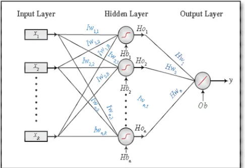
The extension of the single-layer feed-forward structure to the multilayer feed-forward structure as depicted in Fig. 1. As it can be seen, that there are still exist the input layer of nodes and the output layer of nodes as in the single-layer case. However, between these two layers are one or more layers of nodes known as a hidden layer. All these layers of nodes are denoted as layer 0 (input layer), layer 1 (first hidden layer), layer 2 (second hidden layer), and finally layer M (output layer) [3].
Until this date, multilayer feed-forward network or also known as MLP has become the major and most widely used supervised learning neural network architecture [4]. Since MLPs utilize computationally intensive training algorithms (such as the error back-propagation), then this algorithm can easily get stuck in local minima. In addition, this architecture has problems in dealing with large amounts of training data, while demonstrating poor interpolation properties, when using reduced training sets [4]. In addition, attention also must be drawn to the use of biases. Basically, neurons can be chosen with or without biases. Since the bias gives the network extra variable, then it logically translates that the networks with biases would be more powerful [4].
Fig. 1 Feed Forward Neural Network with one hidden layer and one output layer
There are different types of ANNs existing, and their uses are very high in many applications. Since the first neural model proposed by McCulloch and Pitts [5], there have been hundreds of different improved models considered as ANNs. The differences between those proposed algorithms might be the functions, the accepted values, the topology, the learning algorithms, etc. Furthermore, there are many hybrid models that had been introduced recently by researchers, where each neuron has more properties, but the focus is directed at an ANN which learns using the back-propagation algorithm [6], [7], [8] for learning the appropriate weights.
Back-Propagation (BP), the most common and popular used neural network learning technique, is one of the most
effective algorithms accepted by most researcher currently, and also the basis of pattern identification of BP neural network. BP algorithm used Gradient-based methods also known as one of the most commonly used error minimization methods used to train back-propagation networks. Despite its popularity, the algorithm still facing some drawbacks such as the defects of local optimal and slow convergence speed [9]. Until then, many research aimed at improving the traditional Back-Propagation Neural Network (BPNN) since 1986 by introducing some additional parameters such as the addition of learning rate, and momentum parameters, or use of different activation function, etc. Moreover, adequately pre-processing the datasets for the neural network before the training the network also influences the performances positively [10]-[14].
Therefore, this study includes analysis and discuss the performance effect of using data pre-processing techniques on back propagation algorithm trained with different algorithms and activation functions. The structure of the paper is highlighted as follows: Section II describes material and method in which focus on the back propagation training algorithm and its improvements. Experimental set up which constitute the data pre-processing techniques, simulations results and analysis are reflected in Section III. The concluding part of Section IV summarizes the contributions of the study.
II. MATERIAL AND METHOD
The back-propagation (BP) algorithm has recently emerged as one of the most efficient learning procedures for multi-layer networks, and it also is known as one of the most common algorithms used in the training of artificial neural networks [15]-[19]. The BP learning has become efficient with the establishment of its mathematical formula as the standard method or process in adjusting weights and biases for training an ANN in many domains [20]. The formulation of the back-propagation algorithm can be defined as follows: By given a set of testing data that was propagated to the MLP then its start to calculate the output as follows;
hi= f
∑
x wi ij (1)yi = f
∑
h wi jk (2)where h is the hidden node, x is the input need, w is the weight, and y is the output node. The BP training algorithm is an iterative gradient algorithm designed to minimize the mean square error between the actual output of a multilayer feed-forward perceptron and the desired output. In this case, once the output is calculated then the network will start to compute the error, which will be the difference of the expected value t and the actual value, and compute the error information term δ for both the output and hidden nodes.
δ
h
i=
h
i(1
−
h
i).
δ
y w
i.
jk (3)
δ
h
i=
h
i(1
−
h
i).
δ
y w
i.
jk (4)Once the information errors for each node were calculated, then, the network will back-propagate this error through the network by adjusting all of the weights; starts from the weights to the output layer and ends at the weights to the input layer.
∆
w
jk=
ηδ
.
y h
i.
i(5)
∆ =
w
ijηδ
.
h x
i.
i (6)wnew = ∆ +w wold (7)
where η is the learning rate.
The generally good performance found for the BP algorithm is somewhat surprising considering by many researchers, and the applications of Artificial Neural Network with Back Propagation algorithm have gained immense popularity in different areas. Some of these areas include but not limited to: voice recognition, face detection, control systems, medical, cause and effect analysis, engineering, time series prediction, and cryptosystems, etc.
The Multilayer Perceptron (MLP) training is an iterative process the most common method used to train MLP is the back-propagation (BP) algorithm for classification. The basic process in BP algorithm is that at each epoch the calculation of the network outputs patterns in the training set the adjustment was made to the network weights according to the difference between actual network output and the desired output. This BP algorithm has been independently derived by several researchers working in different fields, and the algorithm has the capacity of organizing the representation of the data in the hidden layers with high power of generalization [15].
The BP algorithm implements the gradient descent method which is the most venerable, but also one of the least effective, classical optimisation strategies. The process of updating the weights can be done using either a batch method or an on-line method. For batch training method, weight changes are accumulated over an entire presentation of the training data (epoch) before being calculated, while for on-line training method, the weights were updated after the presentation of each training example (instance). Hence, until today, Back Propagation Gradient Descent (GD) is probably the simplest of all learning algorithms usable for training multi-layered neural networks. Even though it is not the most efficient algorithm, but it converges fairly reliably. Furthermore, the calculation equations were already well established. This well-established technique is often attributed to Rumelhart, Hinton, and Williams [5].
The main focus of BP training algorithm is to reduce the error function by iteratively adjusting the network weight vectors. In training, for each iteration, the weight vectors are adjusted one layer at a time from the output level towards the network inputs. That is why, in the gradient descent version of BP, the change in the network weight vector in each layer happens in the direction of the negative gradient of the error function with respect to each weight itself. Hence, from that process, it can be noted that the introduction of learning rate η is multiplied by the negative
of the gradient to conclude the changes to the weights and biases.
Moreover, another parameter had also played an important part in BP training, and it is known as momentum. The back-propagation with momentum algorithm (GDM) has been largely analysed in the neural network literature and even compared with other methods which are often trained by the use of gradient descent with momentum. Normally, a momentum term is usually included in the simulations of connectionist learning algorithms. It is proved and well known that such a term greatly improves the speed of learning, where the used of momentum can speed up and stabilize the training iteration procedure for the gradient method. A momentum term is often added to the increment formula for the weights, in which the present weight updating increment combined the present gradient of the error function and the previous weight updating increment.
( )
. .
.
(
1)
ij j ij ij
w r
ηδ
x
α
w r
∆
=
+ ∆
−
(8)where α is the momentum parameter, and r is the of iteration The momentum parameter can be an analogy of the mass of Newtonian particles that moves through a viscous medium in a conservative force field. Therefore, this paper identified that the performance of GDM depends on two training parameters. One is the parameter learning rate which is similar to the simple gradient descent. The other one is the parameter momentum which is a constant that defines the amount weights changes.
Even though the BP algorithm has proved satisfactory results when applied to many training tasks, but despite many successful applications, the BP algorithm has several important limitations. Since the BP algorithm uses the gradient descent method to update weights, one of the limitations of this method is that it is not guaranteed to find the global minimum of the error function. The problem of improving the learning efficiency and convergence rate of the BP algorithm has been investigated by a number of researchers. One approach had been proposed to incorporate learning rate adaptation methods and apply the Goldstein-Armijo line search in Back-Propagation algorithms [21]. It was found out that the advantages of using these methods are because they provide stable learning, robustness to oscillations, and improved convergence rate. The experiments reveal that the algorithms proposed can ensure to reach global convergence (that is avoiding local minima).
Since the sigmoid derivative which appears in the error function of the original BP algorithm has a bell shape, it sometimes causes slow learning progress when the output of a unit is near ‘0’ or ‘1’. That is why the importance of activation function within the back propagation algorithm was emphasized in the work done by Sibi et al. [22]. They carried out a performance analysis by choosing different activation functions, and confirmed that the choice of selecting activation functions play a great role in the performance of the neural network; other parameters also come into play such as training algorithms, network sizing, and learning parameters.
network output units. It is well known that the activation function (also called a transfer function) can be a linear or nonlinear function. In addition, the activation function f(.) is also known as a squashing function where it keeps the cell’s output between certain limits as is the case in the biological neuron [21]. On the other hand, the relationship between the net inputs and the output is joined and called the activation function of the Artificial Neuron. There could be different kind of function or relationships that determine the value of output that would be produced for given net inputs. Furthermore, there are different types of activation functions [22], and the Uni-Polar Sigmoidal Function (S-shape function) and Hyperbolic Tangent Function.
However, a sigmoid function is by far the most common form of an activation function used in the construction of artificial neural networks [15]. The formula of the activation function of the Uni-polar sigmoid function is given as follows:
( ) 1( )
1 x
g x
e− =
+ (9) There are many advantages of using this function especially in neural networks trained by back-propagation algorithms. First of all, this function can be easily distinguished, and this can interestingly minimize the computation capacity for training. The term sigmoid devoted ‘S-shaped’, and logistic form of the sigmoid maps where the interval (-∞, ∞) onto (0, 1) [18] as seen in Fig. 2.
In other applications, the other choice of activation function is selected such that the output y is in the range from -1 to +1 rather than 0 to +1 [22]. Hence, that activation function is known as hyperbolic tangent function and can be represented diagrammatically in Fig. 2. The equation that defined the ratio between the hyperbolic sine and the cosine functions or expanded as the ratio of the half difference and the half sum of two exponential functions in the points x and –x as follows:
tanh( ) sin( ) cosh( )
x x
x x
x e e
x
x e e
−
− −
= =
+ (10)
Fig. 2 The unipolar sigmoidal function (S-shaped) and the hyperbolic tangent function
Among various attempts to enhance the efficiency of BP algorithm that has been mentioned before, those using the gain value are among the easiest to implement. Shortly after the finding on the gain, researchers had paid their attention to the parameters that influence the performance of BP training is known as gain value. In general, the value of the gain parameter, c , which directly influenced the slope of
the activation function [23]. It was found out that for a large gain values (
c
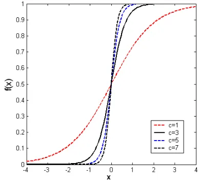
>>1), the activation function nearly approaches a ‘step function’ whereas for a small gain values (0 <c
<< 1), the output values change from zero to closely unity over a large range of the weighted sum of the input values and the sigmoid function approximates a ‘linear function’ as shown in Fig. 3.Fig. 3 The effect of gain on sigmoid activation function
It has been recently shown that a BP algorithm using a variation of gain in an activation function converges faster that the standard BP algorithm. The main reason for such improvement on the BP was that the gain value adequately causes a change in the momentum and learning rate [23].
There were many simulation results that showed the use of changing gain propels the convergence behaviour and also slide the network through local minima. This including in the area of pattern recognition, the identification and recognition of complex patterns by the adjustment of weights experimented upon [24]-[25]. It is proved from the experimental results that by using the gain value, it yielded high accuracy and better tolerance factor, but may take a considerable amount of time. The research was taken into next level by Nawi et al. [26] who proposed a cuckoo search optimized method for training the back propagation algorithm. The simulation results showed that the performance of the proposed method proved to be more effective based on convergence rate, simplicity, and accuracy.
A. Data Processing Technique
confusing results. Thus, the representation and quality of data are first and foremost before running any analysis [27]. It is important in data analysis research to consider the quality, reliability and availability are some of the factors that may lead to a successful data interpretation by a neural network. Furthermore, if there is inappropriate information present or noisy and unreliable data, then knowledge discovery process becomes very difficult during the training process.
It is known to all data analysis researchers that data preparation and filtering steps can take a considerable amount of processing time but once pre-processing is done, the data become more reliable and robust results are achieved [28]. Therefore, as part of improving the training efficiency of BP algorithm, this study had employed three pre-processing techniques namely; Min-Max Normalization (Equation 11), Z-Score Normalization (Equation 12), and Decimal Scaling Normalization (Equation 13).
(
)
min
' _ max _ min _ min
max min
p
p p p
p p
d
d = − new −new +new
− (11)
where maxpis the maximum value of the attribute, minpis
the minimum value of the attribute for (
p
new_max –
p
new min_ ) = 0. When (maxp–minp) = 0, it indicates a constant value for that feature in the data.
' ( ) ( ) d mean p d
std p −
= (12)
The mean(p) translate to the mean of attribute P, and std(p) represents the standard deviation of attribute P.
' 10m
d
d = (13)
where m is the smallest integer such that Max(|d’|) < 1.
III.RESULTS AND DISCUSSION
Experiments had been set up and performed to provide the empirical evidence on the comparative study of different data pre-processing methods in MLP Back Propagation model for classification problems. Two different training algorithms and two different activation functions were selected. The programming code was developed by using MATrix LABoratory (MATLAB) which implements the algorithms. Some selected datasets have been retrieved from the UCI Machine Learning Repository namely: Iris plant data, Balance-Scale data, and Car Evaluation dataset. The data partition for training algorithms is split into 70% for the training set and 30% for the testing set for all the datasets. Whereas, parameters values for η and α which are used with standard Gradient Descent (GD) and Gradient Descent with Momentum (GDM) with all the datasets are η = 0.1 - 0.7 (only for GD), and (α and η) = 0.1 – 0.7 (for GDM).
The performance analyses are performed across 10 trials, where the averages of all trials were recorded. The effect of having data pre-processing techniques with ANN training algorithm is evaluated based on simulations with some
benchmark datasets. The evaluation of the pre-processing techniques coupled with different activation functions by using various training algorithms such as GD and GDM. Towards the end of the simulations, the target outcome of the simulations is to know the ability of each model whether they can perform best with three evaluations performance in consideration. They performance criteria for the analysis are the classification accuracy (ACC) and Mean Squared Error (MSE) depicted in Equation (14) and Equation (15).
In addition, the numbers of Epoch (i.e. the number of times of all the training vectors that are used once to update the weights) make up the third metrics with values set at 5000. If the model performs well and reaches the targets, then it can then be applied to new data to predict the future.
ACC=(C A/ ) *100 (14)
where (C) represent the corrected class, and (A) the total
number of instance.
MSE 1
(
Pi Pi*)
n=
∑
− (15)where Pi is a vector of (n) predictions, Pi* is the vector of the true values, and n is the number of instances.
The simulation experiments are carried out using MATLAB (R2012a) on Petium4 Core i7 CPU, and all results after series of experiments are tabulated and discussed.
The pre-processing techniques on training algorithm GD and GDM with different activation functions (tansig = hyperbolic tangent and logsig = sigmoidal) for MLP have been applied on iris dataset, which contains 150 instances, partitioned into a training set and testing set, with a distribution of 70% and 30% respectively. The network is built with one hidden layer; and for GD, the learning rate was initially started with 0.1, and increasing by 0.2 until it reached a maximum of 0.7. When GDM is concerned, the best learning rates are chosen from previous experience, but momentum was initially started with 0.1, and increasing by 0.2 until it reached a maximum of 0.7. The number of outputs is 3 nodes each for the training algorithms.
TABLEI
CLASSIFICATION PERFORMANCES FOR IRIS DATASET
Pre-processing techniques- Activation
functions
Learning Rate
(η)
GD
Momentum (α)
(η=0.3, 0.5)
GDM ACC
(%)
MSE (%)
ACC (%)
MSE (%)
Min-Max - Tansig
0.1 0.3 0.5 0.7
95.38 96.22 96.78 94.80
0.027 0.019 0.016 0.015
0.1 0.3 0.5 0.7
97.80 95.16 97.23 95.73
0.018 0.017 0.018 0.016
Min-Max - Logsig
0.1 0.3 0.5 0.7
89.24 95.86 96.03 95.68
0.113 0.073 0.059 0.067
0.1 0.3 0.5 0.7
95.43 95.87 95.66 95.37
0.033 0.094 0.045 0.023 Decimal Scaling – Tansig 0.1
0.3 0.5 0.7
87.69 95.61 96.68 96.57
0.059 0.029 0.029 0.022
0.1 0.3 0.5 0.7
95.26 96.05 94.96 94.72
0.024 0.023 0.024 0.024 Decimal Scaling – Logsig 0.1
0.3 0.5 0.7
86.53 94.31 93.04 89.08
0.118 0.076 0.049 0.086
0.1 0.3 0.5 0.7
92.37 88.31 91.37 93.18
0.087 0.088 0.096 0.095
Z-Score - Tansig
0.1 0.3 0.5 0.7
96.47 96.41 97.59 96.60
0.013 0.012 0.011 0.012
0.1 0.3 0.5 0.7
96.82 96.59 95.96 97.86
0.012 0.011 0.010 0.012
Z-Score - Logsig
0.1 0.3 0.5 0.7
97.33 97.76 96.72 92.79
0.054 0.028 0.021 0.044
0.1 0.3 0.5 0.7
96.91 97.14 95.41 97.99
0.019 0.035 0.032 0.025
The results obtained from the classification accuracy based on balance-scale dataset varied proportionally to pre-processing techniques, as shown in Table 2. However, for all pre-processing techniques on training algorithm (GD) with different activation functions (tansig and logsig), 0.5 learning rate gave the highest possible accuracy but Z-Score-Logsig with the highest accuracy. The Z-Score-Tansig with 0.5 learning rate outperformed the other pre-processing techniques in terms of minimum error. On GDM training algorithm, Z-Score-Tansig with momentum at 0.5 and learning rate of 0.5 accounted for the highest accuracy. Consequently, Z-Score-Tansig also gave the lowest error of 0.037% at momentum rate of 0.7.
The performance results as revealed in Table 3 for car evaluation data illustrates that the pre-processing techniques
TABLEII
CLASSIFICATION PERFORMANCES FOR BALANCE SCALE DATASET
Pre-processing techniques- Activation
functions
Learning Rate
(η)
GD Momentum (α)
(η= 0.5) GDM ACC (%) MSE (%) ACC (%) MSE (%)
Min-Max – Tansig
0.1 0.3 0.5 0.7 91.16 89.88 93.84 93.75 0.068 0.061 0.053 0.055 0.1 0.3 0.5 0.7 90.52 91.76 92.63 92.55 0.054 0.057 0.057 0.049
Min-Max - Logsig
0.1 0.3 0.5 0.7 83.19 93.30 94.74 94.47 0.108 0.060 0.053 0.049 0.1 0.3 0.5 0.7 94.18 94.59 94.45 94.85 0.053 0.053 0.053 0.052
Decimal Scaling – Tansig
0.1 0.3 0.5 0.7 85.23 89.80 92.76 92.41 0.094 0.072 0.059 0.063 0.1 0.3 0.5 0.7 92.84 91.76 91.63 90.33 0.067 0.061 0.069 0.068
Decimal Scaling – Logsig
0.1 0.3 0.5 0.7 82.98 87.62 91.02 89.69 0.117 0.083 0.068 0.057 0.1 0.3 0.5 0.7 85.84 92.89 90.01 87.77 0.086 0.067 0.083 0.080
Z-Score – Tansig
0.1 0.3 0.5 0.7 93.61 92.84 94.26 93.85 0.049 0.047 0.039 0.044 0.1 0.3 0.5 0.7 92.84 94.70 95.41 93.33 0.044 0.039 0.038 0.037
Z-Score - Logsig
0.1 0.3 0.5 0.7 94.19 95.06 95.58 95.48 0.059 0.047 0.043 0.046 0.1 0.3 0.5 0.7 94.98 95.39 94.81 95.38 0.042 0.047 0.046 0.047
TABLEIII
CLASSIFICATION PERFORMANCES FOR CAR EVALUATION DATASET
Pre-processing techniques- Activation
functions
Learning Rate
(η)
GD
Momentum (α)
(η= 0.1,0.5) GDM ACC (%) MSE (%) ACC % MSE %
Min-Max - Tansig
0.1 0.3 0.5 0.7 95.88 96.38 96.64 96.57 0.185 0.071 0.067 0.066 0.1 0.3 0.5 0.7 96.35 96.07 96.11 96.06 0.063 0.066 0.065 0.066
Min-Max - Logsig
0.1 0.3 0.5 0.7 96.43 96.24 96.22 96.16 0.121 0.094 0.086 0.084 0.1 0.3 0.5 0.7 96.13 96.18 96.35 95.95 0.109 0.123 0.118 0.118
Decimal Scaling – Tansig 0.1 0.3 0.5 0.7 96.16 96.24 96.31 96.14 0.095 0.086 0.082 0.149 0.1 0.3 0.5 0.7 96.26 96.61 96.46 96.40 0.095 0.102 0.091 0.089
Decimal Scaling – Logsig 0.1 0.3 0.5 0.7 96.17 96.29 96.31 95.64 0.119 0.107 0.099 0.106 0.1 0.3 0.5 0.7 96.11 96.25 96.32 95.92 0.195 0.106 0.107 0.111
Z-Score - Tansig
0.1 0.3 0.5 0.7 96.30 96.15 96.29 96.21 0.073 0.064 0.061 0.059 0.1 0.3 0.5 0.7 96.35 96.25 95.86 96.33 0.060 0.060 0.061 0.062
Z-Score - Logsig
IV.CONCLUSION
Motivated by the re-occurrence of the Back Propagation (BP) neural network sticking to local optimal, convergence speed, and the increase in computational cost associated with its learning process, this study explored the influence of data pre-processing at alleviating the BP shortcomings. Taking advantage of the Min-Max, Decimal Scaling, and Z-Score pre-processing techniques, coupled with the gradient descent and gradient descent with momentum training algorithms and activations functions; uni-polar sigmoidal and hyperbolic tangent, the performances of BP neural network are greatly improved with minimum errors. The experimental results align with the projected goal of this study. For all the datasets at different learning rates and momentum, the pre-processing techniques increased the accuracy of the BP classifier with Z-Score outperforming the other techniques. Also, the computational cost diminishes which ultimately increase performance. Hence, it can be concluded that adequately pre-processing that data optimizes the overall efficiency of the neural network.
ACKNOWLEDGMENT
The authors would like to thank Universiti Tun Hussein Onn Malaysia (UTHM) Ministry of Higher Education (MOHE) Malaysia for financially supporting this Research under Trans-displinary Research Grant Scheme (TRGS) vote no. T003. This research also supported by GATES IT Solution Sdn. Bhd under its publication scheme.
REFERENCES
[1] Mokhlessi, O., Rad, H.M., Mehrshad, N.: Utilization of 4 types of Artificial Neural Network on the diagnosis of valve-physiological heart disease from heart sounds. Biomedical Engineering (ICBME), 2010 17th Iranian Conference of. pp. 1–4 (2010)
[2] Nicoletti, G.M.: Artificial neural networks (ANN) as simulators and emulators-an analytical overview. Intelligent Processing and Manufacturing of Materials, 1999. IPMM’99. Proceedings of the Second International Conference on. pp. 713–721 (1999)
[3] Bhuiyan, M.Z.A.: An algorithm for determining neural network architecture using differential evolution. Business Intelligence and Financial Engineering, 2009. BIFE’09. International Conference on. pp. 3–7 (2009)
[4] Penedo, M.G., Carreira, M.J., Mosquera, A., Cabello, D.: Computer-aided diagnosis: a neural-network-based approach to lung nodule detection. Med. Imaging, IEEE Trans. 17, 872–880 (1998)
[5] McCulloch, W.S., Pitts, W.: A logical calculus of the ideas immanent in nervous activity. Bull. Math. Biophys. 5, 115–133 (1943) [6] Psichogios, D.C., Ungar, L.H.: A hybrid neural network-first
principles approach to process modeling. AIChE J. 38, 1499–1511 (1992)
[7] Choon Sen Seah, Shahreen Kasim, Mohd Saberi Mohamad: Specific Tuning Parameter for Directed Random Walk Algorithm Cancer Classification. International Journal on Advanced Science, Engineering and Information Technology, Vol. 7 (2017) No. 1, pages: 176-182
[8] Moaath Shatnawi, Mohammad Faidzul Nasrudin, Shahnorbanun Sahran: A new initialization technique in polar coordinates for Particle Swarm Optimization and Polar PSO. International Journal on Advanced Science, Engineering and Information Technology, Vol. 7 (2017) No. 1, pages: 242-249
[9] Si-Jun, T.: System Optimal Design Approach using Knowledge-Based Genetic Neural Networks. J. Appl. Sci. 14, 82–88 (2014) [10] Nawi, N.M., Atomi, W.H., Rehman, M.Z.: The Effect of Data
Pre-processing on Optimized Training of Artificial Neural Networks. Procedia Technol. 11, 32–39 (2013)
[11] Filimon, D.-M., Albu, A.: Skin diseases diagnosis using artificial neural networks. Applied Computational Intelligence and Informatics (SACI), 2014 IEEE 9th International Symposium on. pp. 189–194 (2014)
[12] Li, H., Yang, D., Chen, F., Zhou, Y., Xiu, Z.: Application of Artificial Neural Networks in Predicting Abrasion Resistance of Solution Polymerized Styrene-Butadiene Rubber Based Composites. arXiv Prepr. arXiv1405.5550. (2014)
[13] Isa, I.S., Saad, Z., Omar, S., Osman, M.K., Ahmad, K.A., Sakim, H.A.M.: Suitable MLP network activation functions for breast cancer and thyroid disease detection. Computational Intelligence, Modelling and Simulation (CIMSiM), 2010 Second International Conference on. pp. 39–44 (2010)
[14] Dan, Z.: Improving the accuracy in software effort estimation: Using artificial neural network model based on particle swarm optimization. Service Operations and Logistics, and Informatics (SOLI), 2013 IEEE International Conference on. pp. 180–185 (2013)
[15] Günther, F., Fritsch, S.: neuralnet: Training of neural networks. R J. 2, 30–38 (2010)
[16] Basu, J.K., Bhattacharyya, D., Kim, T.: Use of artificial neural network in pattern recognition. Int. J. Softw. Eng. its Appl. 4, (2010) [17] Ghazali, R., Hussain, A.J., Al-Jumeily, D., Lisboa, P.: Time series
prediction using dynamic ridge polynomial neural networks. Developments in eSystems Engineering (DESE), 2009 Second International Conference on. pp. 354–363 (2009)
[18] Badri, L.: Development of Neural Networks for Noise Reduction. Int. Arab J. Inf. Technol. 7, 289–294 (2010)
[19] Lahmiri, S.: A comparative study of backpropagation algorithms in financial prediction. Int. J. Comput. Sci. Eng. Appl. 1, (2011) [20] Nawi, N.M., Khan, A., Rehman, M.Z.: A New Levenberg Marquardt
Based Back Propagation Algorithm Trained with Cuckoo Search. Procedia Technol. 11, 18–23 (2013)
[21] Magoulas, G.D., Vrahatis, M.N., Androulakis, G.S.: Improving the convergence of the backpropagation algorithm using learning rate adaptation methods. Neural Comput. 11, 1769–1796 (1999) [22] Sibi, M.P., Ma, Z., Jasperse, C.P.: Enantioselective addition of
nitrones to activated cyclopropanes. J. Am. Chem. Soc. 127, 5764– 5765 (2005)
[23] Hamid, N.A., Nawi, N.M., Ghazali, R., Salleh, M.N.M.: Improvements of Back Propagation Algorithm Performance by Adaptively Changing Gain, Momentum and Learning Rate. Int. J. New Comput. Archit. their Appl. 1, 866–878 (2011)
[24] Kaur, A., Monga, H., Kaur, M.: Performance Evaluation of Reusable Software Components. Int. J. Emerg. Technol. Adv. Eng. 2, (2012) [25] Seung, S.: Multilayer perceptrons and backpropagation learning.
9.641 Lect. 1–6 (2002)
[26] Rehman, M.Z., Nawi, N.M.: The effect of adaptive momentum in improving the accuracy of gradient descent back propagation algorithm on classification problems. Communications in Computer and Information Science 179 Part 1, 454-459, (2011)
[27] Sibi, P., Jones, S.A., Siddarth, P.: Analysis Of Different Activation Functions Using Back Propagation Neural Networks. J. Theor. Appl. Inf. Technol. 47, 1344–1348 (2013)