Vol.7 (2017) No. 3
ISSN: 2088-5334
Determining the Number of Parallel RC Branches in Polarization/
Depolarization Current Modeling for XLPE Cable Insulation
S. Sulaiman
#, A. Mohd Ariffin
#, D. T. Kien
* #Department of Electrical Power Engineering, Universiti Tenaga Nasional, Jalan IKRAM-UNITEN, Kajang, Selangor, 43000, Malaysia E-mail: [email protected], [email protected]
*
National Load Dispatch Centre, EVN Building, No. 11 Cua Bac Street, Ba Dinh District, Hanoi, 100000, Vietnam E-mail: [email protected]
Abstract— An important element in the electric power distribution system is the underground cable. However continuous applications
of high voltages unto the cable may lead to insulation degradations and subsequent cable failure. Since any disruption to the electricity supply may lead to economic losses as well as lowering customer satisfaction, the maintenance of cables is very important to an electrical utility company. Thus, a reliable diagnostic technique that is able to accurately assess the condition of cable insulation operating is critical, in order for cable replacement exercise to be done. One such diagnostic technique to assess the level of degradation within the cable insulation is the Polarization / Depolarization Current (PDC) analysis. This research work attempts to investigate PDC behaviour for medium voltage (MV) cross-linked polyethylene (XLPE) insulated cables, via baseline PDC measurements and utilizing the measured data to simulate for PDC analysis. Once PDC simulations have been achieved, the values of conductivity of XLPE cable insulations can be approximated. Cable conductivity serves as an indicator of the level of degradation of XLPE cable insulation. It was found that for new and unused XLPE cables, the polarization and depolarization currents have almost overlapping trendlines, as the cable insulation’s conduction current is negligible. Using a linear dielectric circuit equivalence model as the XLPE cable insulation and its corresponding governing equations, it is possible to optimize the number of parallel RC branches to simulate PDC analysis, with a very high degree of accuracy. The PDC simulation model has been validated against the baseline PDC measurements.
Keywords—polarization; depolarization; insulation; XLPE cable; simulation
I. INTRODUCTION
All types of insulation material undergo degradation process or ageing effects. Ageing is fundamentally caused by changes in the molecular structure of the dielectric. There are certain identified parameters that have been defined as ageing factors such as mechanical stress, electrical stress, temperature and environmental factors [1].
Due to the service life of distribution cables, the insulating materials are subject to change. These changes relate to the degradation of the insulation properties of the power cables. The diagnostic technique is a predictive maintenance that can detect the early stage of insulating materials degradation.
Failure of underground cable insulation could affect the whole electrical distribution system. The problems arising from continuous applications of high voltages as well as various ageing mechanisms experiences by the cable insulation can lead to degradation, which reduces the life service of the cable. Therefore, power utility companies are
nowadays faced to choose either to repair, resume as normal or replace the entire cable.
Since the cost of repairing and replacing a degraded underground cable can be very expensive so from a power utility company’s point of view, there is a constant need to allocate its resources strategically to prioritize the cables in accordance with their degradation severity. Thus a “smart cable maintenance” system should be put in place to replace only cables that may affect the electrical network’s reliability [2].
Many non-destructive cable tests have been proposed, amongst which are return voltage method [3]–[5], and dielectric spectroscopy [6]–[9]. Another proposed technique, the Polarization / Depolarization current (PDC) analysis, has been extensively used to assess degradations in machines, power transformers and high voltage insulation system [3], [10]–[16]. There is also a marked interest in recent years to use the PDC analysis to assess for cable insulation degradation [17]–[21].
for the widely used underground cable insulation in service, which is cross-linked polyethylene (XLPE) cables, to a high degree of accuracy, to serve as a starting point towards the determination of conductivity to assess the level of XLPE cable insulation degradation. The study follows the model for linear dielectric circuit equivalence closely, with its corresponding governing equations given in [22], to determine the number of parallel RC branches, n. The method involves using the baseline PDC measurement values on new and unused XLPE cables, to obtain parameters of the governing equations and subsequently determining a suitable value of n.
The determined value of n is then validated against six experimental PDC values. The DC applied voltage, time domain based method used in this study is similar to that used for oil-impregnated paper insulated [13] and metal oxide surge arresters [14], validated against PDC and RVM measurements.
However, this study is unique as it is only to assess for XLPE cable insulation which has different numbers of n and discharging times, when compared to the studies done in [13] and [14], due to the differences in its insulation geometry and type of insulation material. For the purpose of practical modeling, n is within the range of four to ten, subject to its decay pattern of depolarization current [14].
The interpretation of ageing conditions from XLPE cable conductivity values [19], [20] and comparison between PDC and DS techniques [18] to assess for XLPE cable degradations are beyond the scope of this paper and have been reported earlier.
II. MATERIAL AND METHOD
A. PDC Measurement Principles
PDC measurement is conducted by having a DC voltage source applied to the insulation material for a lengthy duration, typically in the range of 1,000 s to 10,000 s. At this voltage application period, current that arises from the charging or polarization process is measured. The magnitude and behaviour of the polarization current are dependent on the conductivity of the insulation. After the charging period has completed, the test sample is then short-circuited, giving rise to an opposite discharging or depolarization current. A schematic of a basic PDC measurement setup is as shown in Fig. 1.
Fig. 1 Basic PDC measurement setup
The typical voltage U(t) and current I(t) profiles across the
insulation, under the application of a step charging voltage
U0, is as per Fig. 2. Both polarization and depolarization
currents, ip and id respectively, are dependent on the
geometry of the insulation [14], [23] and also properties of the insulating material [24], [25]. In the same figure,
tpolarization and tdepolarization refer to the polarization and
depolarization times, respectively.
Fig. 2 Voltage and current profiles across insulation during polarization and depolarization processes [13]
B. Equivalent Circuit
PDC measurements on XLPE cables are performed by measuring the charging and discharging currents when a voltage is applied to the XLPE cable insulation and short-circuited after a long time period. Thus, the insulating medium may be modeled by a circuit equivalence comprising of series connected resistors, R, and capacitors,
C, assigned to parallel RC branches, in order to analyse the
current flow across the insulation. The circuit equivalence is shown below in Fig. 3.
Fig. 3 Equivalent circuit to represent dielectric loss, conduction, and polarization/ depolarization currents across insulation
This equivalent circuit, which is a modified version of the Debye model, is able to simulate polarization and depolarization currents in the time domain. As every parallel
depolarization current is the superposition of these exponentials. The DC resistance R0 represents the
conduction current flowing through the insulation whereas capacitance C0 is used to determine its complex capacitance. C. Governing Equations
Insulation dipoles tend to have an inclination to align themselves to the electric field direction, giving rise to polarization current. The dipoles will relax and return to their previous states once the electric field has been removed. The relaxation process may be represented by parallel RC branches, as shown above in equivalent circuit of Fig. 3. These parallel RC branches which are dependent on the dipoles relaxation characteristics of the insulation corresponds to different time constants, τi.
The insulation bulk resistance, R0 and capacitance C0
depends very much on the XLPE cable geometrical dimension and dielectric properties. They also dictate the amount of conduction current flowing through the insulation.
PDC measurements can be used to determine the circuit parameters. The relationship between polarization, depolarization and conduction currents can generally be expressed as:
ip
( ) ( ) ( )
t =ic t +id t(1)
where ip is charging or polarization current, ic is conduction
current and id is discharging or depolarization current.
Polarization and depolarization currents are both functions of time, made out of a series of exponential decays. Conduction current, on the other hand, should be constant throughout the duration of the voltage application. Expressing the conduction current in terms of Ohm’s law, the following is deduced:
0
0
R U
ic = (2)
where U0 represents the voltage applied across the insulating
material.
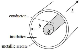
For an XLPE cable, the insulation is between the main current-carrying conductor and the metallic screen, as shown in Fig. 4.
Fig. 4 Simple geometrical representation of an XLPE cable
Thus the bulk resistance R0 and capacitance C0 of the
insulation between the two electrodes can be determined based on the concentric cylinders type of geometry, and also the material properties for the dielectric:
( )
σ πL a b R 2 ln0= (3)
( )
a b L C r ln 2 0 0 ε ε π= (4)
where a is the inner radius of XLPE cable sample insulation,
b is the outer radius of XLPE cable sample insulation, L is
XLPE cable sample length, σ is conductivity and ε0εr is permittivity of insulation material.
The depolarization current consists of a few exponential decays made up of parallel RCbranches and mathematically denoted by: − =
∑
= i n i id A t
i exp τ
1 (5)
with − − = i C i T R U
A 1 exp τ
0
0 (6)
τi=RiCi (7)
where n is a number of parallel RC branches, Ai and τi are
decay constants, and TC is charging time. The respective
values of Ri and Ci in (7) will influence the depolarization
current’s shape of exponential decay. Approximations of decay constants Ai and τi were done using results obtained
from PDC baseline measurements. The determination of n, given in (5), works in conjunction with (6) and (7). The value of n in the simulation is determined by simulating id
for various n values and choosing the n value at which measured and simulated depolarization overlaps each other, to validate their agreement to each other. All the calculations of linear dielectric circuit equivalence model parameters were done using MATLAB.
D. Baseline PDC Measurement Setup
The PDC measurements were performed on six new and unused 11kV medium voltage (MV), XLPE cables with aluminium (Al.) conductor. The cable specifications for the experimental cable samples are as shown in Table 1.
TABLEI
EXPERIMENTAL XLPECABLE SAMPLE SPECIFICATION
Cable Property Specification Cable type 11 kV , 1C XLPE,
Al. conductor Cable manufacturer Tenaga Cable
Industries Sdn. Bhd. Conductor: nominal area 150 mm2 Insulation: thickness 3.4 mm Insulation: inner radius, a 6.9 mm Insulation: outer radius, b 10.3 mm Insulation: relative
permittivity, εr 2.3
shown in Fig. 5, in order to apply the voltage between the insulation.
Fig. 5 Sample of 1 m XLPE cable section, prepared for PDC measurement
For each XLPE cable sample, a DC voltage of 1 kV was supplied for a duration of 1,000 s to enable polarization of the insulation, after which the switch was triggered, and depolarization started, as per basic PDC measurement setup is shown earlier in Fig.1. The polarization and depolarization currents flowing through the insulation were measured with a highly sensitive ammeter of PDC Analyser 1-MOD.
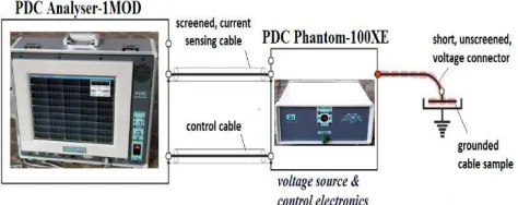
Fig. 6 PDC measurement experimental setup
The experimental setup for the PDC baseline measurement was as shown in the above Fig. 6, consisting of measuring device PDC Analyser 1-MOD, voltage source and control electronics of PDC Phantom-100XE, as well as XLPE cable sample as the test object.
III.RESULTS AND DISCUSSIONS
A. Baseline PDC Measurement
The resulting PDC measured results for all six XLPE cable samples, Cables 1 to 6, were plotted on logarithmic scales and shown in the following Fig. 7 to Fig. 12. All the experimental results showed almost overlapping polarization and depolarization currents. There was no observed difference between the polarization and depolarization currents trendlines, as all the samples were new and unused. Thus no degradation effect due to conduction current was detected, i.e. ic = 0.
The similarity in trendlines between resulting polarization and depolarization currents suggests that without any form of degradation, the circuit parameters describing the polarization and depolarization processes can be treated as almost constant.
Thus the depolarization current results obtained for all six XLPE cables samples can be used to approximate decay constants Ai and τi for the XLPE cable simulation modeling
purposes.
Fig. 7 Polarization and depolarization currents measurements for cable 1
Fig. 8 Polarization and depolarization currents measurements for cable 2
Fig. 10 Polarization and depolarization currents measurements for Cable 4
Fig. 11 Polarization and depolarization currents measurements for Cable 5
Fig. 12 Polarization and depolarization current measurements for cable 6
B. Decay Constants, Ai and τi in PDC Simulation Modeling
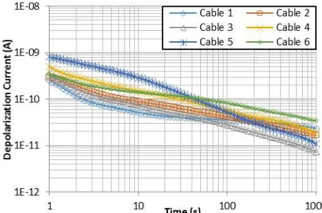
Fig. 13 illustrates the depolarization current for all six XLPE cable samples plotted together in the time domain. It can be observed that the depolarization currents showed no significant difference between one trendline to the other. The negligible variation exhibited may be attributed to the fact that these XLPE cable samples were manufactured by the same cable supplier and had undergone the same cable construction processes. The depolarization currents decayed from around 3–8 nA to around 0.3–8 pA, within the measurement duration.
Fig. 13 Depolarization current plots for all six new, unused baseline PDC measured XLPE cables
The purpose of approximating decay constants, Ai and τi is
to determine the most appropriate number of parallel RC branches, n representing the XLPE cable insulation, with reference to Fig. 3. The depolarization currents from baseline PDC measurement results were taken as a point of reference. The depolarization processes, which are represented by parallel RC branches of the equivalence circuit, estimate the response of the XLPE cable insulation by using distributed relaxation times theory. Dependent on the exponential decay shape of the depolarization current, the value of n varies from four to ten [14].
From the baseline PDC measurement results of depolarization current obtained for the six XLPE cable samples, the sets of data points recorded during the whole measurement period for each sample were determined. Depending on the value of n selected, the depolarization current was then segregated into several segments, as shown in Fig. 14. For example, if the number of RC branches is selected to be 5, then Cable 1, which had 66 data points for the duration of 1,000 s, will have around 13 data points of depolarization current for each segment.
Fig. 14 Segregation of current according to the number of parallel RC branches, n
Fig. 15 Exponential trend-line obtained from first RiCi branch for cable 1
The expression for the exponential trendline obtained from the first RC branch was then used to simulate the depolarization current for the whole period of measurement.
The simulated values were then subtracted from the actual measurement, leaving current values for the other four RC branches as the first RC branch current would cancel itself with the simulated values.
The same process was repeated to find the exponential function representing the remaining RC branches in order to approximate the values for Ai and τi. Once the values for Ai
and τi were found for each branch current, their corresponding values of Ri and Ci were determined.
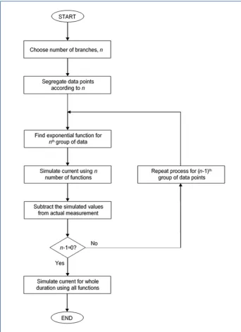
The depolarization current for the insulation can also be simulated as it is made up of the individual current flowing in each branch that has been determined based on the number of branches, n selected. The overall procedure for computing the simulation modeling of PDC can be summarized in the flowchart, shown in Fig. 16.
C. Number of Parallel RC Branches, n in PDC Simulation Modelling
Using the technique given above in part B, the results of current simulation models with different numbers of n against the baseline PDC measurement for Cable 1, were obtained and shown in the following Fig. 17 until Fig. 19.
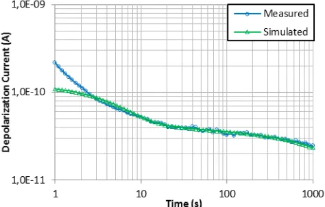
Fig. 17 Comparison between measured and simulated depolarization currents for Cable 1, with n = 4
Fig. 18 Comparison between measured and simulated depolarization currents for Cable 1, with n = 5
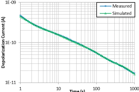
Fig. 19 Comparison between measured and simulated depolarization currents for Cable 1, with n = 6
From these results, it can be seen that the number of parallel RCbranches that is most suitable to represent the current measurement is n = 5 since the result resembles closest to the baseline PDC measurement. For n = 4, the simulation deviates quite significantly from the baseline
PDC measurement, and when n = 6, there was a slight deviation in the early region of the depolarization current. The simulation was also attempted using n = 7, but the result obtained differs significantly from the baseline PDC measurement and therefore will not be discussed further.
From the optimization of n and simulated depolarization current, the values for decay constants Ai and τi were
obtained using (5) for each parallel RC branch. These decay values were then used to calculate for Ri and Ci values for
each branch using (6) and (7). The Ri and Ci values obtained
for XLPE cable 1 are recorded in the following Table 2.
TABLEII
CABLE 1-PARAMETERS OF Ai,τi , Ri AND Ci
Number of parallel RCBranches, n
5 4 3 2 1
Ri
(Ω/m)
8.64 x 10¹²
1.24 x 10¹⁴
1.11 x 10¹⁴
1.67 x 10¹³
1.67 x 10¹²
Ci
(Fm)
3.86 x 10⁻¹⁰
4.05 x 10⁻¹²
2.81 x 10⁻¹³
2.99 x 10⁻¹³
3.86 x 10⁻¹³
D. PDC Comparison between Measured and Simulation Modeling
Similar observations of optimised n = 5, were also obtained for the remaining five XLPE cable samples, Cable 2 until Cable 6, as seen in the following Fig. 20 to Fig. 24.
Fig. 20 Comparison between measured and simulated depolarization currents for Cable 2, with n = 5
Fig. 22 Comparison between measured and simulated depolarization currents for Cable 4, with n = 5
Fig. 23 Comparison between measured and simulated depolarization currents for Cable 5, with n = 5
Fig. 24 Comparison between measured and simulated depolarization currents for Cable 6, with n = 5
Summaries of the Ri and Ci values for the remaining five
XLPE cable samples, Cable 2 to Cable 6, were found to be as per tabulated in Table 3 and Table 4 respectively. These values which were calculated using governing equations of (6) and (7) in MATLAB, influences the exponential decay shape of the simulated polarization currents.
TABLEIII
SUMMARY OF CALCULATED Ri FOR CABLES 2 TO 6
Cable
Resistance per meter for branch i, Ri (Ω/m)
5 4 3 2 1
2 1.50 x 10¹³
3.33 x 10¹³
2.00 x 10¹³
5.00 x 10¹³
3.33 x 10¹²
3 3.16 x 10¹³
3.33 x 10¹³
5.00 x 10¹³
1.11 x 10¹³
1.00 x 10¹²
4 1.26 x 10¹³
1.11 x 10¹³
1.00 x 10¹³
3.33 x 10¹²
1.67 x 10¹¹
5 2.11 x 10¹³
1.00 x 10¹³
5.00 x 10¹²
3.33 x 10¹²
1.67 x 10¹²
6 7.52 x 10¹²
1.43 x 10¹³
3.33 x 10¹³
1.00 x 10¹³
2.00 x 10¹²
TABLEIV
SUMMARY OF CALCULATED Ci FOR CABLES 2 TO 6
Cable Capacitance meter for branch i, Ci (Fm)
5 4 3 2 1
2 1.11 x 10⁻¹⁰
3.75 x10⁻¹²
9.10 x 10⁻¹³
9.56 x 10⁻¹⁴
3.90 x 10⁻¹³
3 3.16 x 10⁻¹¹
2.73 x 10⁻¹²
5.26 x 10⁻¹³
4.76 x 10⁻¹³
6.06 x 10⁻¹³
4 7.91 x 10⁻¹¹
4.50 x 10⁻¹²
7.69 x 10⁻¹³
4.86 x 10⁻¹³
1.50 x 10⁻¹²
5 4.75 x 10⁻¹¹
7.14 x 10⁻¹²
3.57 x 10⁻¹²
1.85 x 10⁻¹²
6.36 x 10⁻¹³
6 2.21 x 10⁻¹⁰
7.00 x 10⁻¹²
4.47 x 10⁻¹³
2.97 x 10⁻¹³
3.84 x 10⁻¹³
From the PDC simulation comparisons done against new and unused XLPE cable samples, it can thus be hypothesized that the optimal number of parallel RC branches in approximating the equivalent circuit parameters for these XLPE cable samples is n = 5, for a 1,000 s duration of the current measurement.
This is consistent with what has been reported in [14] that the optimal number of parallel RC branches can vary from 4 up to 10, dependant on the duration of measurement of insulation test object and decay pattern of its depolarization current. For XLPE cable insulation, it has been found to have a shorter measurement duration of 1,000 s instead of the longer measurement durations of 3,000 s and 10, 000 s respectively , found for oil-impregnated paper insulated power transformer [13] and metal oxide surge arrester [14].
IV.CONCLUSIONS
performed to analyze conditions of insulation for oil-impregnated paper insulated power transformers and metal oxide surge arrester, instead of XLPE cables, and the duration of PDC measurement were set for durations of 3,000 s and 10,000 s respectively, instead of 1,000 s. Therefore, it can be deduced that the type and geometry of insulation under study, and the duration measurement may to some extent dictate the ideal number of parallel RC branches required to represent the linear dielectric circuit equivalence.
The proposed PDC simulation has been validated against the baseline PDC measurements to a very high precision level, seen by the almost overlapping measured and simulated depolarization current trendlines in all six XLPE cable samples.
ACKNOWLEDGMENT
We extend our appreciation to Tenaga Nasional Berhad Research Sdn. Bhd. (TNBR) for providing the necessary equipment, material, and premise for conducting the experiment.
REFERENCES
[1] E. F. Steennis and F. H. Kreuger, “Water Treeing in Polyethylene Cables,” IEEE Trans. Electr. Insul., vol. 25, no. 5, pp. 989–1028, 1990.
[2] M. Dakka, A. Bulinski, and S. Bamji, “On-site diagnostics of medium-voltage underground cross-linked polyethylene cables,” IEEE Electr. Insul. Mag., vol. 27, no. 4, 2011.
[3] B. Jonuz, P. H. F. Morshuis, H. J. Van Breen, J. Pellis, and J. J. Smit, “Detection of water trees in medium voltage XLPE cables by return voltage measurements,” 2000 Annu. Rep. Conf. Electr. Insul. Dielectr. Phenom. Cat No00CH37132, vol. 1, pp. 355–358, 2000.
[4] R. Patsch and J. Jung, “Improvement of the Return Voltage Method for Water Tree Detection in XLPE,” in IEEE Int. Symp. Elect. Insul., 2000, pp. 133–136.
[5] C. S. Pispiris, “Cable Diagnosis. In-situ Tests With Returned Voltage Diagnosis Method in Romania,” in CIRED2001, 2001, no. 482, pp. 18–21.
[6] A. Helgeson and U. Gafvert, “Dielectric response measurements in time and frequency domain on high voltage insulation with different response,” Proc. 1998 Int. Symp. Electr. Insul. Mater. 1998 Asian Int. Conf. Dielectr. Electr. Insul. 30th Symp. Electr. Insul. Mater. (IEEE Cat. No.98TH8286), pp. 393–398, 1998.
[7] P. Werelius, “Development and Application of High Voltage Dielectric Spectroscopy for Diagnosis of Medium Voltage XLPE Cables,” Royal Institute of Technology (KTH), Sweden, 2001. [8] W. S. Zaengl, “Dielectric spectroscopy in time and frequency domain
for HV power equipment. I. Theoretical considerations,” IEEE Electr. Insul. Mag., vol. 19, no. 5, pp. 5–19, 2003.
[9] W. S. Zaengl, “Applications of dielectric spectroscopy in time and frequency domain for HV power equipment,” IEEE Electr. Insul. Mag., vol. 19, no. 6, pp. 9–22, 2003.
[10] S. A. Bhumiwat, “Depolarization index for dielectric aging indicator of rotating machines,” IEEE Trans. Dielectr. Electr. Insul., vol. 22, no. 6, pp. 3126–3132, 2015.
[11] S. Bhumiwat, S. Lowe, P. Nething, J. Perera, P. Wickramasuriya, and P. Kuansatit, “Performance of oil and paper in transformers based on IEC 61620 and dielectric response techniques,” IEEE Electr. Insul. Mag., vol. 26, no. 3, pp. 16–23, 2010.
[12] S. D. Flora, M. S. Divekar, and J. S. Rajan, “Factors Affecting Polarization and Depolarization Current Measurements on Insulation of Transformers,” IEEE Trans. Dielectr. Electr. Insul., vol. 24, 1, no. February, pp. 619–629, 2017.
[13] T. K. Saha, M. K. Pradhan, and J. H. Yew, “Optimal time selection for the polarisation and depolarisation current measurement for power transformer insulation diagnosis,” 2007 IEEE Power Eng. Soc. Gen. Meet. PES, pp. 1–7, 2007.
[14] T. K. . and Saha and K. P. Mardira, “Modeling metal oxide surge arrester for the modern polarization based diagnostics,” IEEE Trans. Dielectr. Electr. Insul., vol. 12, no. 6, pp. 1249–1258, 2005. [15] M. K. Pradhan, J. H. Yew, and T. K. Saha, “Influence of the
geometrical parameters of power transformer insulation on the frequency domain spectroscopy measurement,” IEEE Power Energy Soc. 2008 Gen. Meet. Convers. Deliv. Electr. Energy 21st Century, PES, pp. 1–8, 2008.
[16] M. A. Talib, N. A. Muhamad, and Z. A. Malek, “Fault classification in power transformer using polarization depolarization current analysis,” 2015 IEEE 11th Int. Conf. Prop. Appl. Dielectr. Mater., pp. 983–986, 2015.
[17] S. A. Bhumiwat, “On-site non-destructive diagnosis of in-service power cables by Polarization / Depolarization Current analysis,” in Proceedings of IEEE International Symposium on Electrical Insulation, 2010, pp. 1–5.
[18] A. Mohd. Ariffin, S. Sulaiman, A. Z. C. Yahya, and A. B. A. Ghani, “Analysis of cable insulation condition using dielectric spectroscopy and polarization / depolarization current techniques,” in 2012 IEEE International Conference on Condition Monitoring and Diagnosis, 2012, pp. 145–148.
[19] S. Sulaiman, A. M. Ariffin, and D. T. Kien, “Comparing simulation modelling and measurement results of polarization/depolarization current analysis on various underground cable insulation systems,” in Proceedings of IEEE International Conference on Solid Dielectrics, ICSD, 2013, pp. 137–140.
[20] S. Sulaiman, A. Mohd Ariffin, and D. T. Kien, “Simulation modeling of polarization and depolarization current analysis for underground cable insulation,” Proc. 2013 IEEE 7th Int. Power Eng. Optim. Conf. PEOCO 2013, no. June, pp. 358–361, 2013.
[21] G. Ye, H. Li, F. Lin, J. Tong, X. Wu, and Z. Huang, “Condition assessment of XLPE insulated cables based on polarization/depolarization current method,” IEEE Trans. Dielectr. Electr. Insul., vol. 23, no. 2, pp. 721–729, 2016.
[22] E. Kuffel, W. S. Zaengl, and J. Kuffel, “High Voltage Engineering, Fundamentals,” High Volt. Eng., vol. 1, no. c, p. 552, 2001. [23] S. K. Ojha, P. Purkait, and S. Chakravorti, “Modeling of relaxation
phenomena in transformer oil-paper insulation for understanding dielectric response measurements,” IEEE Trans. Dielectr. Electr. Insul., vol. 23, no. 5, pp. 3190–3198, 2016.
[24] S. A. Bhumiwat, “Insulation condition assessment of transformer bushings by means of polarisation/depolarisation current analysis,” in Conference Record of the 2004 IEEE International Symposium on Electrical Insulation, 2004, no. September, pp. 19–22.