M E T H O D O L O G Y
Open Access
How sample size can effect landslide size
distribution
Langping Li
1, Hengxing Lan
1,2*and Yuming Wu
1Abstract
Background:Landslide size distribution is widely found to obey a negative power law with a rollover in the smaller size, and has been exploited by many researchers to inspect landside physics or to assess landslide erosion and landslide hazard. Yet, sample size has effect on the statistics of landslide size even though we manage to avoid complications associated with landslide datasets and statistical treatments.
Results:In this paper, a series of stochastic simulations were implemented to explicitly and systematically quantify the effect of sample size. The results show that, the errors of parameters estimated based on small sample size can be considerably large. For a sample size of 100, the relative error of the estimated landslide erosion rate that has a probability of 50 % can approach 100 %. In addition, small sample size also obscures the statistical significance of the variances in parameters between different subsets of the same dataset. Although inconsistency was found regarding how the power exponent varies with rainfall intensity, numerical results suggest that the variance observed in a dataset with a small sample size may be not statistically significant.
Conclusions:This paper not only reveals the potential effect of sample size on exploiting landslide size distribution but also presents procedures for quantifying this issue in future studies.
Keywords:Landslide size distribution, Sample size, Statistical significance, Power law, Rollover
Background
The frequency of landslide is widely observed to decrease as a power law with the increase of size after a maximum value (Stark and Hovius 2001; Malamud et al. 2004; Brunetti et al. 2009). This partial power law behav-ior is unique because it is represented by not only a heavy tail as observed in many phenomena (Caers et al. 1999; Cheng 2008; Pinto et al. 2012; Kolyukhin and Tveranger, 2014), but also a rollover in the smaller size. The exponent of the power law tail (γ) and the rollover (R) are therefore the two most characteristic parameters. On one hand, landslide size distribution is crucial for quantitative analysis of landslide hazard (Hungr et al. 1999; Guzzetti et al. 2005) and earth surface processes
(Hovius et al. 1997; Larsen and Montgomery 2012). On the other hand, the emergence of the power law tail and the rollover are mysteries that still lack widely accepted physical explanations (Pelletier et al. 1997; Katz and Aharonov 2006; Stark and Guzzetti 2009; Lehmann and Or 2012; Frattini and Crosta 2013; Alvioli et al. 2014; Li et al. 2014 and references therein). Therefore, landslide size distribution has been exploited by many researchers either to inspect the physics of landslides or to assess landslide erosion and landslide hazard.
The statistics of landslide size could be obscured by complications associated with landslide datasets and statistical treatments in the first place. The following strategies had been adopted to mitigate these compli-cations: 1) using event-based rather than historical landslide datasets (Malamud et al. 2004; Ghosh et al. 2012); 2) using the same dataset prepared by the same author instead of datasets prepared by different authors (Iwahashi et al. 2003; Guzzetti et al. 2008; * Correspondence:[email protected]
1State Key Laboratory of Resources and Environmental Information System,
Institute of Geographic Sciences and Natural Resources Research, Chinese Academy of Sciences, 11A, Datun Road, Chaoyang District, Beijing 100101, China
2Department of Civil and Environmental Engineering, University of Alberta,
Edmonton, Canada
Chen 2009); and 3) using the maximum likelihood estimation (MLE) rather than linear regression to estimate both the power exponent and the rollover (Fiorucci et al. 2011; Ghosh et al. 2012). Nevertheless, even without these complications, limited sample size can also cast a shadow on the statistics of landslide size. Sample size effect is in fact a problem faced by many disci-plines (Lazzeroni and Ray 2012). The error on the esti-mated scaling parameter of power law distributions from sample size effects has been investigated (Clauset et al. 2009). Yet, the potential effect of sample size on the statis-tics of landslide size has not been explicitly addressed. The fact that small differences in parameters of the size fre-quency relationship may produce huge mismatches in the derived landslide erosion rates (Korup et al. 2012) suggests the significance of this issue in some respects. This paper aims to quantitatively inspect the possible effect of sample size on exploiting landslide size distribution. We will focus on the landslide area distribution because so far no satis-factory distribution function for landslide volume has been proposed and most empirical datasets do not have landslide volume data.
Methods
Landslide area distribution
The widely adopted double Pareto function (Stark and Hovius 2001) and Inverse Gamma function (Malamud et al. 2004) were used to characterize the landslide area distributions. And parameters of the two distributions were estimated by the maximum likelihood estimation (MLE). It is inconclusive whether the two functions are mathematically and physically eligible to represent the landslide area distributions in the real world, but they are a practical choice since there are capable of characterizing both the power law tail and the rollover of landslide area distribution. To examine the assumption that landslide size distribution is characterized by a power law tail goes beyond the topic of this paper, we therefore did not test that hypothesis. For the same reason, we did not examine whether log-normal function (ten Brink et al. 2009; Mackey and Roering 2011), logarithmic function (Issler et al. 2005; Che et al. 2011) or exponential function (Montgomery et al. 1998) is an alternative to characterize the empirical data of landslide size. Analytical distribution function for landslide area yielded by maximizing Tsallis entropy (Chen et al. 2011) were not used as it is accom-panied by complications (Li et al. 2012).
The expression of the double Pareto distribution is:
pdpð Þ ¼A β
tð1−δÞ
1þðm=tÞ−α
½ β=α
1þðA=tÞ−α
½ 1þβ=αðA=tÞ
−α−1 ð 1Þ
where
δ¼ 1þðm=tÞ−α
1þð Þc=t −α
β=α
ð2Þ
A is landslide area, pdp(A) is probability density of
landslide area, α, β, andt are constants, while cand m
are two cutoffs define the interval within which the normalization condition satisfies. This function can be approximated by a negative power law (tail) with an ex-ponent of -α-1 for large size events and a positive power law with an exponent ofβ-1 for small size events sepa-rated by a maximum (rollover). With the maximum probability density, we have the rollover at area value:
RAdp¼ exp 1
αðlnðβ−1Þ−lnðαþ1ÞÞ þ lnt
ð3Þ
We therefore do not usetas the“crossover”ofpdp(A)
as suggested by Stark and Hovius (2001), but use the area with maximum probability density as the“rollover”. We chose 1 and 1010as the two cutoffs to ensure all the landslide area values in empirical datasets fall into this scope and found similar choices (e.g., 1 and 108) get al-most the same estimates of parameters.
The expression of the Inverse Gamma distribution is:
pigð Þ ¼A 1
aΓ ρð Þ a A−s
h iρþ1
exp − a
A−s
h i
ð4Þ
whereAis landslide area,pig(A) is probability density of landslide area, Γ(ρ) is the gamma function of ρ, whileρ,
a, and s are constants. The normalization condition is satisfied within [s, +∞). This function can be approxi-mated by a negative power law (tail) with an exponent of -ρ-1 for large size events and an exponential function for small size events separated by a maximum (rollover). With the maximum probability density, we have the roll-over at area value:
RAig¼
a
ρþ1þs ð5Þ
Average landslide volume
The landslide volume (V) is found to relate to landside
area (A) with a scaling exponent τ and an intercept ε
(Guzzetti et al. 2009; Larsen et al. 2010; Klar et al. 2011) such that:
V Að Þ ¼εAτ ð6Þ
Then, an average landslide volume (Va) can be defined
and calculated by:
Va¼ Z
V Að Þp Að ÞdA¼
Z
within which the normalization condition satisfies. The average volume is important because it leads to the amount of landslide erosion and further the landslide erosion rate if the total landslide number is given. In other words, Eq. (6) makes it possible to inspect how the parameter estimation of landslide area distribution affects the estimation of landslide erosion rate. In our study, the relationship V= 2.59A1.05 deduced from the Fujian historical landslide inventory (Li et al. 2014) is used, and Eq. (y6) is calculated numerically.
Stochastic simulation
A straightforward procedure is designed to inspect the effect of sample size on the reliability of the parameter estimation of landslide size distribution. It is assumed that: 1) the theoretical distribution of landslide size with respect to a certain event within a certain area is constrained by physical factors and is therefore predeter-mined; 2) the number of landslides occurring in a certain event within a certain area is finite; and 3) the size of each individual occurred landslide is stochastic. So, we firstly introduce a predefined theoretical
distribu-tion of landslide area, and then draw N values of area
from the theoretical distribution using Monte Carlo simulation, whereNis the sample size. Values of sample size span from 100 to 10,000 and are logarithmic spaced. With regard to each sample size, 1,000 Monte Carlo samples are produced to reveal the stochasticity of the estimated parameters. If the sample size is large enough, the estimated parameters of the 1,000 Monte Carlo sam-ples are expected to have a mean value similar to the parameters of the theoretical distribution and a low standard deviation. On the contrary, if the sample size is small, a mean value far different to the theoretical value and a high standard deviation are expected.
Similarly, we also use a straightforward way to inspect how the sample size influences the statistical significance of the comparison of the parameters of landslide size distribution between different subsets. Firstly, with re-gard to each sample size, the sample with parameters most similar to the theoretical values is picked out from the formerly produced 1,000 Monte Carlo samples as the test sample for this sample size. Then, for each sam-ple size, the corresponding test samsam-ple is randomly sub-divided into two subsets according to a subdividing ratio. And six subdividing ratios, namely 1:1, 2:1, 3:1, 4:1, 5:1, and 6:1, are used to inspect the effect of subdiv-iding ratio as well. For each test sample, the random subdivision is repeated 1,000 times for each subdividing ratio. If we take“the observed differences in parameters between the two subsets are attributed to random
pro-cesses” as the null hypothesis, the region of rejection
and also the region of acceptance for a certain signifi-cance level (e.g., 0.05) can be estimated according to the
statistics of the variances in parameters observed in the 1,000 random trials.
Landslide dataset
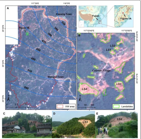
Heavy rainfall struck Fujian in the mid-to-late June, 2010 and induced large numbers of landslides. The
Xiayang-Wangtai (XW as an abbreviation) area, for which SPOT
images with 2.5 m spatial resolution taken shortly after this rainfall event are available (Fig. 1), suffered greatly from this rainfall event. Rainfall records show that the
cu-mulative rainfall in the XW area in this period exceeds
300 mm and approaches 600 mm (Fig. 1a). Landslides in the study area were manually mapped on the SPOT im-ages in a GIS platform. The bright brownish area repre-senting both the failure and the deposition zones were visually delineated as fresh landslide areas (Fig. 1b). Field reconnaissance had helped to link real landslide scenarios with features on the SPOT images (Fig. 1c, d, e). In addition, the topography was inspected through a digital elevation model (DEM) with 5 m spatial resolution to support the mapping. The brownish area in gullies that represents the traces of debris flows and floods were not delineated. As seen during field surveys, shallow earth slides account for most of the landslides in theXWarea in this event. Totally 12,524 landslides were identified in the study area which means a density of about 43 landslides per square kilometer. We will refer to this inventory as “XWdataset”.
The high resolution of the SPOT images and DEM im-plies that this event-based landslide dataset ought to be substantially complete for landslides with area larger than 25 m2regarding this rainfall event within thisXW
area. In addition, only one interpreter was involved in the mapping procedures. This suggests that potential er-rors due to the diversity of the skills and experience of the interpreters are avoided in the following statistical
analysis. Two subsets of theXW dataset, namelyR1 and
R2, were produced according to the 450 mm cumulative
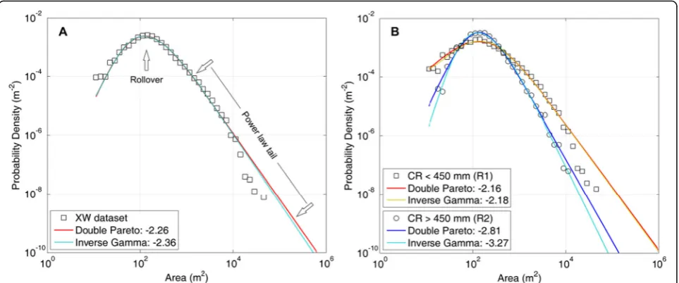
rainfall isoline as shown in Fig. 1a. The probability distri-butions of landslide area fitted to the empirical datasets using MLE are shown in Fig. 2. The statistical parame-ters, including the estimated exponents of the power law tail (γ) and the estimated rollovers (R), are presented in Table 1. In the following analysis, we will take the fitted landslide size distributions of theXWdataset as the pre-defined theoretical distributions for the Monte Carlo simulations, and will also test whether the observed
vari-ances in parameters between the R1 and R2 subsets is
statistically significant or not.
Results
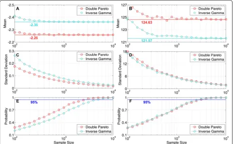
The reliability of estimating parameters
presented in Fig. 3. For both the double Pareto distribu-tion and the Inverse Gamma distribudistribu-tion, as sample size gets smaller, the mean of the estimated parameters gets more deviated from the theoretical value (Fig. 3a, b) while the standard deviation gets larger (Fig. 3c, d). In addition, the probability that the estimated value has a relative error less than 5 % is calculated to quantify the performance of parameter estimation. Not surprisingly, for both the exponent and the rollover, this probability decreases
dramatically as sample size gets smaller (Fig. 3e, f). Com-pared with the Inverse Gamma distribution, the estimated exponents using the double Pareto distribution have lower standard deviations. Therefore, the performance of the double Pareto distribution on estimating the exponent is relatively better than the Inverse Gamma distribution (Fig. 3e). On the contrary, on estimating the rollover, the performance of the Inverse Gamma distribution is slightly better than the double Pareto distribution (Fig. 3f).
If we take 95 % as a rule of thumb (Fig. 3e, f ), the minimum sample size required for reliable parameter es-timation can be inferred. However, finding a threshold universally applicable is unrealistic. It is related to not only the distribution function but also the theoretical parameters. Numerical experiments show that larger theoretical parameters (absolute values) require larger sample size to guarantee a high probability of low relative error. Nevertheless, Fig. 3 shows that 6,000 is a roughly safe choice for most landslide datasets. In view of this standard, utilizations of the parameters esti-mated based on small sample size, for example less than 1,000 (Fiorucci et al. 2011; Ghosh et al. 2012; Regmi et al. 2014), especially for quantitative use (Larsen and Montgomery 2012; Tsai et al. 2013), should be
cautious. We will specifically inspect how sample size affects the reliability of landslide erosion estimates in the discussion.
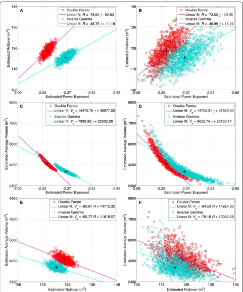
The shape of landslide size distribution is defined by all the parameters, although the power law tail and the rollover are the two most characteristic features. As both double Pareto function and Inverse Gamma function have three variables, a good estimation of one parameter cannot guarantee a good estimation of another param-eter. Thus, it is necessary to inspect the correlations between the estimated parameters besides inspecting them separately. The correlations between the estimated power exponents, rollovers and average volumes for sample size 10,000 and 1,000 are presented in Fig. 4. Generally, larger power exponents (absolute values) come with larger rollovers, while the average volume is inversely proportional to the power exponent (absolute value) and the rollover. Although these trends are distinct, scattering is also obvious in the plots. The less scattered results of larger sample size suggests more reliable estimates.
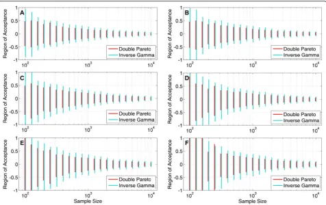
The statistical significance of comparing parameters
The regions for accepting the null hypothesis that “the
differences in parameters between two different subsets of the same landslide dataset are derived from stochastic
processes” are shown in Figs. 5 and 6 forγ and R,
re-spectively. The significance level is 0.05, and the differ-ences in parameters are the results of the parameters of the subsets with larger sample size subtracting that of the subsets with smaller sample size. Narrower region of
Fig. 2Probability distributions of landslide area fitted to theXWdataset using the maximum likelihood estimation are shown. The scattered open squares and circles showing the empirical data represent the probability densities estimated based on histogram with logarithmic bins. Numerical values indicate the scaling exponents of the fitted power law tails.aThe entireXWdataset.bThe two subsets of theXWdataset identified according to cumulative rainfall
Table 1Statistical characteristics of landslide dataset and subsets
Dataseta Nb Areac(m2) Double Pareto Inverse Gamma
Min Max Mean γd Re(m2) γ R(m2)
XW 12,524 8 48,846 695 −2.26 124.63 −2.36 121.57
R1 6,297 8 48,846 1,021 −2.16 133.82 −2.18 137.85
R2 6,227 18 10,224 365 −2.81 136.33 −3.27 128.49
a
Dataset:“XW”indicates the entireXWdataset,“R1”and“R2”indicate subsets of theXWdataset characterized by a cumulative rainfall of lower and higher than 450 mm, respectively
bN
: number of landslides in a dataset (sample size)
c
Area:“Min”,“Max”and“Mean”indicate the minimum, maximum and mean landslide area of a dataset respectively
d
γ: scaling exponent of the power law tail of the landslide area probability distribution fitted using the maximum likelihood method
eR
acceptance means we have wider region of rejection in which we are confident in attributing the observed vari-ances in parameters to physical constraints other than random processes.
It is shown that, regardless of distribution function, for bothγandR, as sample size gets smaller or subdividing ratio gets larger, the region of acceptance gets wider (worse). It means smaller sample size and larger subdiv-iding ratio expect larger differences in parameters to be observed for the sake of statistical significance. It also shows that the double Pareto distribution performs bet-ter on estimating the exponent (Fig. 5) while the Inverse Gamma distribution performs slightly better on estimat-ing the rollover (Fig. 6). The regions of acceptance go beyond the range of figures for sample sizes less 250 if the subdividing ratio is large. This is because small sam-ple size together with large subdividing ratio will yield unrealistic wide regions of acceptance. For example, with regard to a sample size of 100 and a subdividing ratio of
5, the regions of acceptance for γ estimated using the
double Pareto distribution and the Inverse Gamma dis-tribution are [−14.69, 13.75] and [−18.22, 15.24], respect-ively. Therefore, comparing the parameters of different subsets of a landslide dataset with an extreme small
sample size, for instance less than 100 (Iwahashi et al. 2003), is practically statistically meaningless.
Numerical experiments show that, for the same sam-ple size and subdividing ratio, larger parameters (abso-lute values) of the“mother dataset”yields wider regions of acceptance. Therefore, it is hard to find a universal standard for statistical significance. It is also hard to tell whether some published variances in parameters be-tween different subsets is statistical significant or not, because either the MLE is not used (Chen 2009) or the information is not sufficient (Guzzetti et al. 2008). Nevertheless, test of statistical significance is highly recommended prior to physical interpretations of the variation of landslide size distribution between different subsets, especially for those with small sample size (Santangelo et al. 2013; Guns and Vanacker 2014). In the discussion, we will show that small sample size can cast a shadow on interpreting the physical constraints on landslide size distribution.
Discussion
The proposed statistical procedures in this paper is of potential use for exploiting landslide size distribution, in-cluding such as estimating landslide erosion rate, assessing
Fig. 3The statistical characteristics of the estimated power exponents (γ) and rollovers (R) regarding different sample size are presented.aMean ofγ.bMean ofR.cStandard deviation ofγ.dStandard deviation ofR.eThe probability that the estimatedγhas a relative error less than 5 %.
landslide hazard and inspecting the physics of landslides. In this section, the effect of sample size on estimating landslide erosion rate is specifically discussed, and an example is presented to show that sample size can affect the confidence in attributing the variation of landslide size distribution to the spatial heterogeneity of rainfall intensity.
The estimation of landslide erosion rate
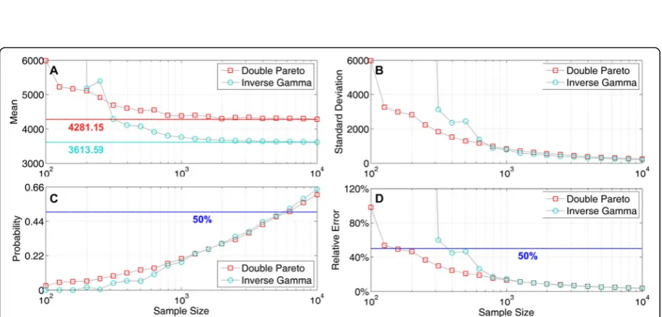
The statistical characteristics of the estimated average volume (Va) with respect to each sample size are
pre-sented in Fig. 7. Similar to the power exponent and roll-over, as sample size gets smaller, the mean of the
estimated Va gets more deviated from the theoretical
value (Fig. 7a) while the standard deviation gets larger (Fig. 7b). However, the potential error of volume estima-tion is more significant compared with that of the power exponent and rollover. This can be seen from the prob-ability that the estimated value has a relative error less than 5 % (Fig. 7c). A sample size of 6,000 can only guar-antee a probability of about 50 % that the estimated Va
has a relative error less than 5 %. The relative error of the estimatedVathat has a probability equal to 50 % is
also calculated (Fig. 7d). It shows that, for the double Pareto distribution and Inverse Gamma distribution re-spectively, when sample size gets around 150 and 350, there will be half a chance that the estimated Va has a
relative error of 50 %. The double Pareto distribution performs relatively better on estimating the average vol-ume than the Inverse Gamma distribution. However, even for the double Pareto distribution, there will be a probability of 50 % that the estimated Va has a relative
error near 100 % if the sample size is 100 (Fig. 7d). As landslide erosion rate is positively proportional to aver-age landslide volume, the error of estimatingVawill
dir-ectly bring the same error to the estimation of landslide erosion rate. In similar way, the potential error of asses-sing landslide hazard caused by insufficient sample size can be estimated, given the relationship between land-slide size and landland-slide intensity is provided.
The variation of landslide size distribution with rainfall intensity
The significance of the observed variances inγandR
be-tween the two subsets (R1 and R2) of the XW dataset
(Table 1) had been tested. We randomly subdivide the
Fig. 6The regions of acceptance for the null hypothesis that“the observed differences in rollover (R) between two different subsets of the same dataset is derived from random processes”at a significance level of 0.05 are shown.a,b,c,d,eandfpresent the results for subdividing ratio 1:1, 2:1, 3:1, 4:1, 5:1 and 6:1, respectively. Please note that the lower bounds of region of acceptance for sample sizes near 100 go beyond the range of this picture (less than−100) when the subdividing ratio is 5:1 or 6:1
Fig. 7The statistical characteristics of the estimated average landslide volume (Va) regarding different sample size are presented.aMean ofVa.
12,524 landslides into two subsets with 6,297 and 6,227 landslides respectively for 1,000 times. The results show that, all the differences in parameters observed between theR1 andR2 subsets is statistical significant at a signifi-cant level of 0.05, except for the difference in rollover
es-timated using the double Pareto distribution (−2.51),
which has a significant level of about 0.21. Therefore, from the conservative point of view, we attribute the observed variances in rollover to random processes but suggest a physical explanation for the variances in power exponent.
We find that larger cumulative rainfall produces a steeper power law tail of the landslide area distribution (Fig. 2b). This is opposite to the previously reported result that the power law tail becomes flatter with an increase of the cumulative rainfall (Chen 2009). The variation of power exponent with rainfall intensity is essential because it concerns the problem whether increased rainfall intensity will increase the relative pro-portion of small size landslides or large size landslides. The explanation of this disagreement goes beyond the scope of this paper. Instead, we suggest a test of signifi-cance prior to physical interpretation. However, the stat-istical significance of the result published by Chen (2009) cannot be exactly told since the MLE was not used. Nevertheless, a variance of power exponent 0.27 is obtained by subdividing a landslide dataset with a sam-ple size less than 600. This result falls into the region of acceptance according to our numerical experiments (Fig. 4). Therefore, from a statistical point of view, there may be no adequate confidence to exclude the possibility that the variance of power exponent with rainfall intensity observed in Chen (2009) is due to random processes.
Conclusions
A series of numerical experiments were implemented in this paper to systematically quantify the effect of sample size on exploiting landslide area distribution. The results show that, as sample size gets smaller, both the reliability of the parameter estimation and the statistical signifi-cance of the variances in parameters observed between different subsets get worse. Therefore, quantitative ana-lysis of landslide hazard and land surface erosion based on the statistics of landslide dataset with small sample size may be accompanied by considerable errors. Specif-ically, with a sample size of 100, the relative error of the estimated landslide erosion rate that has a probability of 50 % can approach 100 %. Furthermore, inconsistency was found regarding how the power exponent of land-slide area distribution varies with rainfall intensity. Our numerical results suggest that the variance observed in a dataset with a small sample size may be not statistically significant. Although this study had focused on landslide
area distribution and adopted the double Pareto distribu-tion and the Inverse Gamma distribudistribu-tion, the presented procedures can be also used to quantify the potential effects of sample size regarding landslide volume distribu-tion and other distribudistribu-tion funcdistribu-tions.
Nevertheless, because the results of numerical simula-tions are affected by the statistical characteristics of the concerned landslide dataset, it is hard to find universally applicable criteria for adequate (large enough) sample size. A design for testing the potential effects of sample size on landslide size statistics but not a rule of thumb was proposed in this paper. It must be emphasized that, only larger sample size cannot guarantee reliable statis-tical results, a landslide dataset with physically represen-tative sample distribution is usually a prerequisite.
Acknowledgments
This research was supported by National Natural Science Foundation of China (NO. 41525010, 41272354 and 41472282) and Research Foundation for Youth Scholars of IGSNRR, CAS. The authors also wish to thank Fujian Centre for Geological Environment Monitoring for SOPT images and relevant data. Mr. Zhiwei Wang is particularly appreciated for helping to prepare the landslide dataset in the Xiayang-Wangtai area.
Authors’contributions
LP designed the study, carried out the statistical analysis and drafted the manuscript. HX conceived of the study, and participated in its design and coordination and helped to draft the manuscript. YM participated in the statistical analysis. All authors read and approved the final manuscript.
Competing interests
The authors declare that they have no competing interests.
Received: 2 July 2016 Accepted: 4 October 2016
References
Alvioli, M., F. Guzzetti, and M. Rossi. 2014. Scaling properties of rainfall-induced landslides predicted by a physically based model.Geomorphology213: 38–47. Brunetti, M.T., F. Guzzetti, and M. Rossi. 2009. Probability distributions of landslide
volumes.Nonlinear Proc Geophys16(2): 179–188.
Caers, J., J. Beirlant, and M.A. Maes. 1999. Statistics for modelling heavy tailed distributions in geology: Part I. Methodology.Mathematical Geoscience31(4): 391–410. Che, V.B., M. Kervyn, G.G.J. Ernst, P. Trefois, S. Ayonghe, P. Jacobs, E. van Ranst,
and C.E. Suh. 2011. Systematic documentation of landslide events in Limbe area (Mt Cameroon Volcano, SW Cameroon): geometry, controlling, and triggering factors.Natural Hazards59(1): 47–74.
Chen, C.Y. 2009. Sedimentary impacts from landslides in the Tachia River Basin, Taiwan.Geomorphology105(3–4): 355–365.
Chen, C.C., L. Telesca, C.T. Lee, and Y.S. Su. 2011. Statistical physics of landslides: New paradigm.EPL95(4): 49001.
Cheng, Q.M. 2008. Non-linear theory and power-Law models for information integration and mineral resources quantitative assessments.Mathematical
Geoscience40: 503–532.
Clauset, A., C.R. Shalizi, and M.E.J. Newman. 2009. Power-law distributions in empirical data.SIAM Review51(4): 661–703.
Fiorucci, F., M. Cardinali, R. Carlà, M. Rossi, A.C. Mondini, L. Santurri, F. Ardizzone, and F. Guzzetti. 2011. Seasonal landslide mapping and estimation of landslide mobilization rates using aerial and satellite images.Geomorphology 129(1–2): 59–70.
Frattini, P., and G.B. Crosta. 2013. The role of material properties and landscape morphology on landslide size distributions.Earth and Planetary Science Letters 361: 310–319.
Guns, M., and V. Vanacker. 2014. Shifts in landslide frequency–area distribution after forest conversion in the tropical Andes.Anthropocene6: 75–85. Guzzetti, F., P. Reichenbach, M. Cardinali, M. Galli, and F. Ardizzone. 2005. Probabilistic
landslide hazard assessment at the basin scale.Geomorphology72(1–4): 272–299. Guzzetti, F., F. Ardizzone, M. Cardinali, M. Galli, P. Reichenbach, and M. Rossi. 2008.
Distribution of landslides in the Upper Tiber River basin, central Italy.
Geomorphology96(1–2): 105–122.
Guzzetti, F., F. Ardizzone, M. Cardinali, M. Rossi, and D. Valigi. 2009. Landslide volumes and landslide mobilization rates in Umbria, central Italy.Earth and
Planetary Science Letters279(3–4): 222–229.
Hovius, N., C.P. Stark, and P.A. Allen. 1997. Sediment flux from a mountain belt derived by landslide mapping.Geology25(3): 231–234.
Hungr, O., S.G. Evans, and J. Hazzard. 1999. Magnitude and frequency of rock falls and rock slides along the main transportation corridors of southwestern British Columbia.Canadian Geotechnical Journal36(2): 224–238.
Issler, D., F.V. De Blasio, A. Elverhøi, P. Bryn, and R. Lien. 2005. Scaling behaviour of clay-rich submarine debris flows.Mar Petrol Geol22(1–2): 187–194. Iwahashi, J., S. Watanabe, and T. Furuya. 2003. Mean slope-angle frequency
distribution and size frequency distribution of landslide masses in Higashikubiki area, Japan.Geomorphology50(4): 349–364.
Katz, O., and E. Aharonov. 2006. Landslides in vibrating sand box: What controls types of slope failure and frequency magnitude relations?Earth and
Planetary Science Letters247(3–4): 280–294.
Klar, A., E. Aharonov, B. Kalderon-Asael, and O. Katz. 2011. Analytical and observational relations between landslide volume and surface area.Journal
of Geophysical Research116(F02), F02001.
Kolyukhin, D., and J. Tveranger. 2014. Statistical analysis of fracture-length distribution sampled under the truncation and censoring effects.
Mathematical Geoscience46: 733–746.
Korup, O., T. Görüm, and Y. Hayakawa. 2012. Without power? Landslide inventories in the face of climate change.Earth Surf Proc Land37(1): 92–99. Larsen, I.J., and D.R. Montgomery. 2012. Landslide erosion coupled to tectonics
and river incision.Nature Geoscience5(7): 468–473.
Larsen, I.J., D.R. Montgomery, and O. Korup. 2010. Landslide erosion controlled by hillslope material.Nature Geoscience3(4): 247–251.
Lazzeroni, L.C., and A. Ray. 2012. The cost of large numbers of hypothesis tests on power, effect size and sample size.Molecular Psychiatry17(1): 108–114. Lehmann, P., and D. Or. 2012. Hydromechanical triggering of landslides: From
progressive local failures to mass release.Water Resources Research48(3), W03535. Li, L.P., H.X. Lan, and Y.M. Wu. 2012. Comment on“Statistical physics of landslides:
New paradigm”by Chen C.-c. et al.EPL100(2): 29001.
Li, L.P., H.X. Lan, and Y.M. Wu. 2014. The volume-to-surface-area ratio constrains the rollover of the power law distribution for landslide size.Eur Phys J Plus129(5): 89. Mackey, B.H., and J.J. Roering. 2011. Sediment yield, spatial characteristics, and
the long-term evolution of active earthflows determined from airborne LiDAR and historical aerial photographs, Eel River, California.Geological
Society of America Bulletin123(7–8): 1560–1576.
Malamud, B.D., D.L. Turcotte, F. Guzzetti, and P. Reichenbach. 2004. Landslide inventories and their statistical properties.Earth Surf Proc Land29(6): 687–711. Montgomery, D.R., K. Sullivan, and H.M. Greenberg. 1998. Regional test of a
model for shallow landsliding.Hydrological Processes12(6): 943–955. Pelletier, J.D., B.D. Malamud, T. Blodgett, and D.L. Turcotte. 1997. Scale-invariance
of soil moisture variability and its implications for the frequency–size distribution of landslides.Engineering Geology48(3–4): 255–268. Pinto, C.M.A., A. Mendes Lopes, and J.A. Tenreiro Machado. 2012. A review of power
laws in real life phenomena.Commun Nonlinear Sci Numer Simuln17(9): 3558–3578. Regmi, N.R., J.R. Giardino, and J.D. Vitek. 2014. Characteristics of landslides in
western Colorado, USA.Landslides11(4): 589–603.
Santangelo, M., D. Gioia, M. Cardinali, F. Guzzetti, and M. Schiattarella. 2013. Interplay between mass movement and fluvial network organization: An example from southern Apennines, Italy.Geomorphology188: 54–67. Stark, C.P., and F. Guzzetti. 2009. Landslide rupture and the probability distribution of
mobilized debris volumes.Journal of Geophysical Research114: F00A02. Stark, C.P., and N. Hovius. 2001. The characterization of landslide size distributions.
Geophysical Research Letters28(6): 1091–1094.
ten Brink, U.S., R. Barkan, B.D. Andrews, and J.D. Chaytor. 2009. Size distributions and failure initiation of submarine and subaerial landslides.Earth and
Planetary Science Letters287(1–2): 31–42.
Tsai, Z.X., G.J.Y. You, H.Y. Lee, and Y.J. Chiu. 2013. Modeling the sediment yield from landslides in the Shihmen Reservoir watershed, Taiwan.Earth Surf Proc Land38(7): 661–674.
Submit your manuscript to a
journal and benefi t from:
7 Convenient online submission 7 Rigorous peer review
7 Immediate publication on acceptance 7 Open access: articles freely available online 7 High visibility within the fi eld
7 Retaining the copyright to your article