Adv. Radio Sci., 7, 133–137, 2009 www.adv-radio-sci.net/7/133/2009/
© Author(s) 2009. This work is distributed under the Creative Commons Attribution 3.0 License.
Advances in
Radio Science
Resolving longitudinal amplitude and phase information of two
continuous data streams for high-speed and real-time processing
A. Guntoro and M. Glesner
Institute of Microelectronic Systems, Department of Electrical Engineering and Information Technology, Technische Universit¨at Darmstadt, Germany
Abstract. Although there is an increase of performance in
DSPs, due to its nature of execution a DSP could not perform high-speed data processing on a continuous data stream. In this paper we discuss the hardware implementation of the amplitude and phase detector and the validation block on a FPGA. Contrary to the software implementation which can only process data stream as high as 1.5 MHz, the hardware approach is 225 times faster and introduces much less la-tency.
1 Introduction
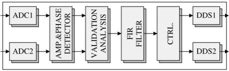
Digital signal processing which replaces the analog control system in our heavy ion acceleration environment is depicted in Fig. 1. Two analog input signals which correspond to the ion states at a specific time are received from the cav-ity sensors and go to the A/D block (with 14-bit resolution at 28.5 MHz sampling rate). Longitudinal amplitude and phase information of both signals are extracted by the detector and go to the validation block. The validation block outputs the longitudinal amplitude and phase differences of both signals. Special phase-corrector filter tunes up the phase of the sig-nal. The corrected signal is used at the end by the controller to control the DDS (Direct Digital Synthesis). In this paper we focus on the amplitude and phase detector and the vali-dation block which should be able to process two high-speed continuous data streams.
Correspondence to: A. Guntoro ([email protected])
2 Longitudinal amplitude and phase
Given a discrete signalf[n], the longitudinal amplitude in-formation of the signal is defined as Iverson (2004); Hind et al. (2003):
χX=
q
x2+y2
and the corresponding longitudinal phase information is φX=arctan
y x
withx=Q1−Q2andy=I1−I2whereI1,I2,Q1, andQ2are the in-phase and quadrature components of the signal.
To resolve the magnitude information, one square root, two square, and one addition operations are involved. Ac-cordingly one division operation and one arctan function are involved to compute the phase.
The magnitude and phase difference of two signals are eas-ily computed with:
χ1=χ1−χ2 φ1=φ1−χ2
Our original implementation of the amplitude and phase de-tector and the validation block which are performed on DSP C6713 is only capable to receive two input data streams as high as 1.5 MHz on each channel Klingbeil (2004). Thus the signals are decimated by 19 which introduces friction and information loss.
2.1 CORDIC
134 A. Guntoro and M. Glesner: Resolving longitudinal amplitude and phase information of two continuous data streams
RESOLVING LONGITUDINAL AMPLITUDE AND PHASE INFORMATION OF TWO
CONTINUOUS DATA STREAMS FOR HIGH-SPEED AND REAL-TIME PROCESSING
Andre Guntoro and Manfred Glesner
Institute of Microelectronic Systems
Department of Electrical Engineering and Information Technology
Technische Universit¨at Darmstadt
email: [email protected], [email protected]
ABSTRACT
Although there is an increase of performance in DSPs, due to its nature of execution a DSP could not perform high-speed data processing on a continuous data stream. In this paper we discuss the hardware implementation of the am-plitude and phase detector and the validation block on a FPGA. Contrary to the software implementation which can only process data stream as high as 1.5 MHz, the hardware approach is 225 times faster and introduces much less la-tency.
1. INTRODUCTION
Digital signal processing which replaces the analog con-trol system in our heavy ion acceleration environment is depicted in Fig. 1. Two analog input signals which corre-spond to the ion states at a specific time are received from the cavity sensors and go to the A/D block (with 14-bit res-olution at 28.5 MHz sampling rate). Longitudinal ampli-tude and phase information of both signals are extracted by the detector and go to the validation block. The validation block outputs the longitudinal amplitude and phase differ-ences of both signals. Special phase-corrector filter tunes up the phase of the signal. The corrected signal is used at the end by the controller to control the DDS (Direct Digital Syn-thesis). In this paper we focus on the amplitude and phase detector and the validation block which should be able to process two high-speed continuous data streams.
ADC1
ADC2
AMP.&PHASE DETECTOR VALIDATION ANALYSIS
FIR
FILTER CTRL.
DDS1
DDS2
Fig. 1. Digital Signal Processing Chain.
2. LONGITUDINAL AMPLITUDE AND PHASE
Given a discrete signalf[n], the longitudinal amplitude in-formation of the signal is defined as [1, 2]:
χX = p
x2+y2
and the corresponding longitudinal phase information is
φX =arctan
y x
withx=Q1−Q2andy=I1−I2whereI1,I2,Q1, andQ2
are the in-phase and quadrature components of the signal. To resolve the magnitude information, onesquare root, twosquare, and oneadditionoperations are involved. Ac-cordingly onedivisionoperation and onearctanfunction are involved to compute the phase.
The magnitude and phase difference of two signals are easily computed with:
χ∆=χ1−χ2 φ∆=φ1−χ2
Our original implementation of the amplitude and phase de-tector and the validation block which are performed on DSP C6713 is only capable to receive two input data streams as high as 1.5 MHz on each channel [3]. Thus the signals are decimated by 19 which introduces friction and information loss.
2.1. CORDIC
The CORDIC (COordinate Rotation DIgital Computer) al-gorithm is a method to compute elementary functions by means of planar rotation and vectoring. The basic of CORDIC principle utilizes only shift and add/sub operations which are simple and cheap from the resource allocation point of view [4]. The coordinate system of the input parameter is rotated through constant angles until the angle is reduced to zero.
Fig. 1. Digital signal processing chain.
parameter is rotated through constant angles until the angle is reduced to zero.
Planar rotation for a vectorAof(Xj, Yj)can be defined in matrix form as:
Xj Yj =
cosθ−sinθ sinθ cosθ
Xi Yi
To calculate the rotation, trigonometric functions (cos and sin) are involved. This rotation angleθ in fact can be exe-cuted in steps by means of iterative process. With a slight rearrangement, Eq. (1) defines this process which performs the rotation stepwise.
Xn+1 Yn+1
=cosθn
1 −tanθn tanθn 1
Xn Yn
(1) By selecting the angle stepsθnsuch that the tangent of a step (tanθn) is a power of 2, the multiplication operation can be eliminated and substituted by shift operation. Equation (2) gives the angle parameter for each step.
θn=arctan
1
2n
(2) Their sums must equal to the rotation angleθ:
∞
X
n=0
Snθn=θ
whereSn={−1; +1}in respect to addition or substraction is determined later. Rewriting Eq. (1), we have:
Xn+1 Yn+1
=cosθn
1 −Sn2−n Sn2−n 1
Xn Yn
Except for the common coefficient cosθn which can be treated as a constantK and computed at the end, multipli-cations are replaced with shift operations.
Residue Z which defines then angle difference between the expected rotation and the iterative rotations is:
Zn+1=θ− n
X
i=0
θi =θ− n
X
i=0
arctan1 2i The rotation parameterSnis determined by:
Sn=
(
−1 ifZn<0 +1 ifZn≥0
Practically, the iteration does not go up to infinity. In the hardware implementation, for each iteration the resolution of the result is increased by one bit (16 iterations deliver 16 bits result). Thus, it is not necesarry to compute the arctan on the fly. Look-up table of 16 entries is enough to store the precomputed arctan values in this case.
DrivingZto zero, the CORDIC performs:
Xj Yj Zj =
P (XicosZi−YisinZi) P (YicosZi+XisinZi)
0
With initial valuesXi=1/P,Yi=0, andZi=θwe will have at the end of the iteration:
Xj Yj Zj = cosθ sinθ 0
To suit our demand, we need to driveY to zero instead of Z. The obtained result is:
Xj Yj Zj = P q
X2i +Yi2 0 Zi+arctan
Yi Xi
Again withXi=X,Yi=Y, andZi=0 we obtain
Xj Yj Zj = P √
X2+Y2 0 arctanYi
Xi (3)
Neglecting the amplification factorP,XjandZjcorrespond to the magnitude and phase information we need.
3 Hardware Realization
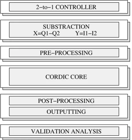
The critical constraint is to process two continuous data streams at a minimum of 28.5 MHz each without introduc-ing any decimation. We exploit a pipeline structure within our design to guarantee this real-time demand. Figure 2 con-cisely depicts the tasks for each pipeline stage.
3.1 2-to-1 controller
This stage receives two input data streams. It collects four samples from each input and feeds them to the subtraction block. To save resources, two input data streams are pro-cessed alternately (i.e. the first clock cycle for the first input, the next clock cycle for the second input and so on).
3.2 Substraction
A. Guntoro and M. Glesner: Resolving longitudinal amplitude and phase information of two continuous data streams 135
Planar rotation for a vector
A
of
(
X
j, Y
j)
can be defined
in matrix form as:
X
jY
j=
cos
θ
−
sin
θ
sin
θ
cos
θ
X
iY
iTo calculate the rotation, trigonometric functions (
cos
and
sin
) are involved. This rotation angle
θ
in fact can be
exe-cuted in steps by means of iterative process. With a slight
rearrangement, Eq. 1 defines this process which performs
the rotation stepwise.
X
n+1Y
n+1= cos
θ
n1
−
tan
θ
ntan
θ
n1
X
nY
n(1)
By selecting the angle steps
θ
nsuch that the tangent of a
step (
tan
θ
n) is a power of 2, the multiplication operation
can be eliminated and substituted by shift operation. Eq. 2
gives the angle parameter for each step.
θ
n= arctan
1
2
n(2)
Their sums must equal to the rotation angle
θ
:
∞
X
n=0
S
nθ
n=
θ
where
S
n=
{−
1; +1
}
in respect to addition or substraction
is determined later. Rewriting Eq. 1, we have:
X
n+1Y
n+1= cos
θ
n1
−
S
n2
−nS
n2
−n1
X
nY
nExcept for the common coefficient
cos
θ
nwhich can be treated
as a constant
K
and computed at the end, multiplications are
replaced with shift operations.
Residue
Z
which defines then angle difference between
the expected rotation and the iterative rotations is:
Z
n+1=
θ
−
n
X
i=0
θ
i=
θ
−
n
X
i=0
arctan
1
2
iThe rotation parameter
S
nis determined by:
S
n=
(
−
1
if
Z
n<
0
+1
if
Z
n≥
0
Practically, the iteration does not go up to infinity. In the
hardware implementation, for each iteration the resolution
of the result is increased by one bit (16 iterations deliver 16
bits result). Thus, it is not necesarry to compute the
arctan
on the fly. Look-up table of 16 entries is enough to store the
precomputed
arctan
values in this case.
Driving
Z
to zero, the CORDIC performs:
X
jY
jZ
j
=
P
(
X
icos
Z
i−
Y
isin
Z
i)
P
(
Y
icos
Z
i+
X
isin
Z
i)
0
With initial values
X
i= 1
/P
,
Y
i= 0
, and
Z
i=
θ
we will
have at the end of the iteration:
X
jY
jZ
j
=
cos
θ
sin
θ
0
To suit our demand, we need to drive
Y
to zero instead
of
Z
. The obtained result is:
X
jY
jZ
j
=
P
p
X
2i
+
Y
2
i
0
Z
i+ arctan
Y
iX
i
Again with
X
i=
X
,
Y
i=
Y
, and
Z
i= 0
we obtain
X
jY
jZ
j
=
P
√
X
2+
Y
20
arctan
Y
iX
i
(3)
Neglecting the amplification factor
P
,
X
jand
Z
jcorre-spond to the magnitude and phase information we need.
3. HARDWARE REALIZATION
The critical constraint is to process two continuous data streams
at a minimum of 28.5 MHz each without introducing any
decimation. We exploit a pipeline structure within our
de-sign to guarantee this real-time demand. Fig 2 concisely
depicts the tasks for each pipeline stage.
X=Q1−Q2
Y=I1−I2
2−to−1 CONTROLLER
SUBSTRACTION
PRE−PROCESSING
CORDIC CORE
POST−PROCESSING
OUTPUTTING
VALIDATION ANALYSIS
Fig. 2
. Pipeline stages of the Amplitude and Phase detector
and Validation Analysis block.
Fig. 2. Pipeline stages of the amplitude and phase detector and validation analysis block.
3.3 Preprocessing
The CORDIC vectoring is only capable of processing the sig-nals arranged on quadrant I and IV. Since the combination of inputsX andY may also lay on quadrant II or III, prepro-cessing and rearrangement of the inputs are necessary. The quadrant preprocessing conversion is formulated as
f0(x, y)=
f (x, y) x ≥0
f (−x,−y)+π x <0, y≥0 f (−x,−y)−π x <0, y <0
which tells that quadrant II is mapped to quadrant IV, thus the result will be corrected by addingπ, and quadrant III is mapped to quadrant I and will be corrected by subtractingπ from the result.
3.4 CORDIC core
The core stage expands the CORDIC iteration into micro pipelines to fulfill our high-speed requirement. 16 pipeline stages are needed to provide 16-bits resolution at the output. To have a full resolution swing, 16-bits two’s complement binary format is used to represent the value between−πand +π for the angle component. LUT-based precalculated arc-tan 2−nis used to store 16 arctan entries. Similar to the angle representation, two’s complement is also used to represent the magnitude component. This is done because the iterative process inside of the core employs also addition and subtrac-tion in estimating the magnitude.
3.1. 2-to-1 Controller
This stage receives two input data streams. It collects four samples from each input and feeds them to the subtraction block. To save resources, two input data streams are pro-cessed alternately (i.e. the first clock cycle for the first input, the next clock cycle for the second input and so on).
3.2. Substraction
This stage handles the extraction of incoming quadrature and in-phase signals into correspondingXandY which will be fed to the CORDIC core. These variables represent di-rectly the vector of which the core operates.
3.3. Preprocessing
The CORDIC vectoring is only capable of processing the signals arranged on quadrant I and IV. Since the combina-tion of inputsX andY may also lay on quadrant II or III, preprocessing and rearrangement of the inputs are necessary. The quadrant preprocessing conversion is formulated as
f′
(x, y) =
f(x, y) x≥0
f(−x,−y) +π x <0, y≥0
f(−x,−y)−π x <0, y <0
which tells that quadrant II is mapped to quadrant IV, thus the result will be corrected by addingπ, and quadrant III is mapped to quadrant I and will be corrected by subtractingπ
from the result.
3.4. CORDIC Core
The core stage expands the CORDIC iteration into micro pipelines to fulfill our high-speed requirement. 16 pipeline stages are needed to provide 16-bits resolution at the output. To have a full resolution swing, 16-bits two’s complement binary format is used to represent the value between−πand
+πfor the angle component. LUT-based precalculated arc-tan 2−n is used to store 16 arctan entries. Similar to the angle representation, two’s complement is also used to rep-resent the magnitude component. This is done because the iterative process inside of the core employs also addition and subtraction in estimating the magnitude.
3.5. Postprocessing and Outputting
The Postprocessing stage corrects the output by adding or subtracting the result withπbased on the information col-lected at the preprocessing stage. Additionally, the amplifi-cation factor which is introduced by CORDIC as defined in Eq. 3 might also be eliminated at this stage if it is demanded. Although it depends on the application, while most appli-cations demand no unity gain correction for the magnitude output.
3.6. Validation Analysis
This stage calculates the difference between two longitudi-nal magnitudes and two longitudilongitudi-nal phases.
4. PERFORMANCE
Three different input sources are utilized to analyze the per-formance of the CORDIC hardware. Fig. 3 depicts these sources. Three cases are considered here: (a) a linear phase and constant magnitude input source, (b) a signal with de-cayingXcomponent and (c) a signal with decayingY com-ponent.
−1−0.8−0.6−0.4−0.2 0 0.20.4 0.60.8 1 −1 −0.8 −0.6 −0.4 −0.2 0 0.2 0.4 0.6 0.8 1
−1−0.8−0.6−0.4−0.2 0 0.2 0.4 0.60.8 1 −1 −0.8 −0.6 −0.4 −0.2 0 0.2 0.4 0.6 0.8 1
−1−0.8−0.6−0.4−0.2 0 0.2 0.40.6 0.8 1 −1 −0.8 −0.6 −0.4 −0.2 0 0.2 0.4 0.6 0.8 1
(a) (b) (c)
Fig. 3. Different test input sources.
Fig. 4 maps the errors (the difference between the ex-pected values and the computed version) of magnitude and phase result of each input source. Here it can be seen that the hardware computation with 16-bit resolution produces the same results with some minor errors compared to the expected results. Tables. 1 and 2 summarize the statistical parameters of the error for both magnitude and phase com-ponents.
Table 1. Maximum error, absolute mean, and standard de-viation of the resulting error for the magnitude component (normalized to 1) for each input source.
Source Max Error |x¯| σ
Const. Mag. 0.000338 0.000111 0.000069 Decaying X 0.000316 0.000118 0.000072 Decaying Y 0.000359 0.000120 0.000072
Table 2. Maximum error, absolute mean, and standard de-viation (all in degree) of the resulting error for the phase component for each input source.
Source Max Error |x¯| σ
Const. Mag. 0.027466 0.007682 0.008817 Decaying X 0.047844 0.007344 0.009223 Decaying Y 0.040306 0.007084 0.008829
Here we can see that by using 16-bit data representation to perform the computation, the introduced errors are
tol-Fig. 3. Different test input sources.
Table 1. Maximum error, absolute mean, and standard deviation of the resulting error for the magnitude component (normalized to 1) for each input source.
Source Max Error |x¯| σ Const. Mag. 0.000338 0.000111 0.000069 Decaying X 0.000316 0.000118 0.000072 Decaying Y 0.000359 0.000120 0.000072
3.5 Postprocessing and outputting
The Postprocessing stage corrects the output by adding or subtracting the result withπ based on the information col-lected at the preprocessing stage. Additionally, the ampli-fication factor which is introduced by CORDIC as defined in Eq. (3) might also be eliminated at this stage if it is de-manded. Although it depends on the application, while most applications demand no unity gain correction for the magni-tude output.
3.6 Validation analysis
This stage calculates the difference between two longitudinal magnitudes and two longitudinal phases.
4 Performance
Three different input sources are utilized to analyze the per-formance of the CORDIC hardware. Figure 3 depicts these sources. Three cases are considered here: (a) a linear phase and constant magnitude input source, (b) a signal with de-cayingXcomponent and (c) a signal with decayingY com-ponent.
136 A. Guntoro and M. Glesner: Resolving longitudinal amplitude and phase information of two continuous data streams
erable. For the magnitude component, the maximum error is in order of3×10−3
; and for the phase component, the maximum phase error does not exceed0.05◦
.
5. SYNTHESIS
The amplitude and phase detector and validation block are written in VHDL. The code has been synthesized using Xil-inx ISE. As the target device, we use XilXil-inx XC2V2000-4 which is employed in our DSP chain. Table. 3 details the re-source usage of the implemented blocks on the target device. It is clear that the implemented block consumes only a small amount of resources and has high operation speed. Due to the pipeline structure, the amplitude and phase detector and the validation block can receive two input data streams as high as 337.78 MHz each (the core operated on 4 samples per clock cycle). Additionally, the computational latency de-termined by the number of pipeline stages (1+1+1+16+2+1=22) is very low (i.e 130 ns).
Table 3. Resource utilization on Xilinx XC2V2000-4. Usage / Cap. Percentage Slices 478 / 10752 4% Flip-Flops 788 / 21504 3% 4 input LUTs 792 / 21504 3% Max. Frequency 168.89 MHz
6. CONCLUSIONS
Contrary to the DSP implementation which is only capable to process data streams as high as 1.5 MHz, the dedicated hardware block is 225 times faster and introduces only a very small amount of computational latency. Thus, the dec-imation by 19 which was taken on our original implementa-tion is no longer required.
7. REFERENCES
[1] J. Iverson, “Digital Control Technology Enhances Power Sys-tem Reliability and Performance,” in Technical Information from Cummins Power Generation. Cummins Power Genera-tion, 2004.
[2] M. Hind, V. Rajan, and P. Sweeney, “Phase shift detection: a problem classification,” inIBM Research Report, 2003.
[3] H. Klingbeil, “A Fast DSP-based Phase-detector for Closed-loop RF Control in Synchrotrons,” IEEE Transaction on In-strumentation and Measurement, 2004.
[4] R. Andraka, “A survey of CORDIC algorithms for FPGA based computers,”FPGA 98 Monterey CA USA, 1998.
−1 −0.8 −0.6 −0.4 −0.2 0 0.2 0.4 0.6 0.8 1 −4
−2 0 2x 10
−4
Magnitude
−1 −0.8 −0.6 −0.4 −0.2 0 0.2 0.4 0.6 0.8 1 −0.03
−0.02 −0.01 0 0.01 0.02
Phase
(a)Constant Magnitude
−1 −0.8 −0.6 −0.4 −0.2 0 0.2 0.4 0.6 0.8 1 −4
−2 0 2x 10
−4
Magnitude
−1 −0.8 −0.6 −0.4 −0.2 0 0.2 0.4 0.6 0.8 1 −0.06
−0.04 −0.02 0 0.02 0.04
Phase
(b)Decaying X Component
−1 −0.8 −0.6 −0.4 −0.2 0 0.2 0.4 0.6 0.8 1 −4
−2 0 2x 10
−4
Magnitude
−1 −0.8 −0.6 −0.4 −0.2 0 0.2 0.4 0.6 0.8 1 −0.06
−0.04 −0.02 0 0.02 0.04
Phase
(c)Decaying Y Component
Fig. 4. The difference between the expected and computed values of every given input source.
Fig. 4. The difference between the expected and computed values of every given input source.
Table 2. Maximum error, absolute mean, and standard deviation (all in degree) of the resulting error for the phase component for each input source.
Source Max Error |x¯| σ Const. Mag. 0.027466 0.007682 0.008817 Decaying X 0.047844 0.007344 0.009223 Decaying Y 0.040306 0.007084 0.008829
Table 3. Resource utilization on Xilinx XC2V2000-4.
Usage/Cap. Percentage Slices 478/10752 4% Flip-Flops 788/21504 3% 4 input LUTs 792/21504 3% Max. Frequency 168.89 MHz
Here we can see that by using 16-bit data representation to perform the computation, the introduced errors are tolerable. For the magnitude component, the maximum error is in or-der of 3×10⁻³; and for the phase component, the maximum phase error does not exceed 0.05◦.
5 Synthesis
The amplitude and phase detector and validation block are written in VHDL. The code has been synthesized using Xil-inx ISE. As the target device, we use XilXil-inx XC2V2000-4 which is employed in our DSP chain. Table 3 details the re-source usage of the implemented blocks on the target device. It is clear that the implemented block consumes only a small amount of resources and has high operation speed. Due to the pipeline structure, the amplitude and phase detector and the validation block can receive two input data streams as high as 337.78 MHz each (the core operated on 4 samples per clock cycle). Additionally, the computational latency deter-mined by the number of pipeline stages (1+1+1+16+2+1=22) is very low (i.e. 130 ns).
6 Conclusions
A. Guntoro and M. Glesner: Resolving longitudinal amplitude and phase information of two continuous data streams 137
References
Andraka, R.: A survey of CORDIC algorithms for FPGA based computers, FPGA 98 Monterey CA USA, 1998.
Hind, M., Rajan, V., and Sweeney, P.: Phase shift detection: a prob-lem classification, in: IBM Research Report, 2003.