M E T H O D O L O G Y
Open Access
Quantifying heterogeneity in individual
participant data meta-analysis with binary
outcomes
Bo Chen
1and Andrea Benedetti
1,2*Abstract
Background: In meta-analyses (MA), effect estimates that are pooled together will often be heterogeneous. Determining how substantial heterogeneity is is an important aspect of MA.
Method: We consider how best to quantify heterogeneity in the context of individual participant data meta-analysis (IPD-MA) of binary data. Both two- and one-stage approaches are evaluated via simulation study. We consider conventionalI2andR2statistics estimated via a two-stage approach andR2estimated via a one-stage approach. We propose a simulation-based intraclass correlation coefficient (ICC) adapted from Goldstein et al. to estimate theI2, from the one-stage approach.
Results: Results show that when there is no effect modification, the estimatedI2from the two-stage model is underestimated, while in the one-stage model, it is overestimated. In the presence of effect modification, the estimatedI2from the one-stage model has better performance than that from the two-stage model when the prevalence of the outcome is high. TheI2from the two-stage model is less sensitive to the strength of effect modification when the number of studies is large and prevalence is low.
Conclusions: The simulation-basedI2based on a one-stage approach has better performance than the conventional I2based on a two-stage approach when there is strong effect modification with high prevalence.
Keywords: Individual participant data meta-analysis (IPD-MA), Heterogeneity, Two-stage and one-stage approaches,I2
Background
Meta-analysis (MA) is a statistical method used to draw an overall conclusion based on the total evidence by review-ing previous research work systematically and poolreview-ing effect estimates together [1]. MA is an important tool, widely used, and applied in evidence-based medicine [2].
Individual participant data meta-analyses (IPD-MA), collect line by line participant data from each included study, rather than estimates of the parameter of inter-est. IPD-MA offer several advantages over aggregate data MA (AD-MA) and are considered the gold standard in meta-analytic techniques [3].
*Correspondence: [email protected]
1Department of Epidemiology, Biostatistics and Occupational Health, McGill University, Purvis Hall, 1020 Pine Avenue West, Montreal, Canada
2Respiratory Epidemiology and Clinical Research Unit, McGill University, 2155 Guy St. 4th Floor, Office 412, 24105 Montreal, Canada
Heterogeneity of effect estimates is an important con-sideration in both AD-MA and IPD-MA. Heterogeneity exists if the true effects vary across studies more than would be expected by chance alone. The estimated inter-study variance (τ2) of the parameter of interest is the most direct measure of heterogeneity, but interpretation, particularly deciding what might be a problematic level of heterogeneity, is difficult, despite some practical sug-gestions [4]. TheI2, originally proposed by Higgins and Thompson, meets three important criteria for any mea-sure of heterogeneity: it monotonically increases with between-study variance; it is not varied by changing the scale; and it is not affected by the number of studies [5]. Importantly, despite some limitations [4], theI2remains the most often reported measure of heterogeneity and is easily interpretable, appealing to clinicians.
There are two approaches to analyze the data from IPD-MA: the two-stage approach and the one-stage approach.
In the two-stage approach, each study is analyzed sepa-rately, then standard meta-analytic techniques are applied, and heterogeneity may be quantified by usual methods. Alternatively, in the one-stage approach, a mixed model is fit and the data is analyzed altogether, accounting for the correlation that may exist between subjects in the same study and allowing the estimated effect to vary across studies. A review of statistical methods used in IPD-MA of binary outcomes found that most do not report any measure of heterogeneity [6]. While some measures of heterogeneity are easily obtained from a one-stage model, the I2 is not. Our objective in this work was to con-sider various approaches to quantifying heterogeneity in IPD-MA of binary outcomes analyzed via the one-stage approach. We propose a method to obtain an I2 from a one-stage model and evaluate it and other possible measures via simulation study.
Metrics of heterogeneity in IPD-MA with binary outcomes
In this section, we describe various measures of hetero-geneity that may be used. Here, we consider that the primary analysis is a one-stage analysis of IPD-MA of dichotomous outcome data. Below, we describe four pos-sible measures of heterogeneity: (1) the conventional I2 from the corresponding two-stage analysis; (2) theRfrom the corresponding two-stage analysis; (3) a new metric: theI2from the one-stage approach; and (4) theRfrom the one-stage approach.
Between-study variance (τ2)
The between-study variance, τ2, quantifies the hetero-geneity in IPD-MA directly. A large value ofτˆ2indicates that heterogeneity exists among the studies. However, the
τ2is not ideal, since interpretation is difficult: there is no standard criteria to determine the level of heterogeneity (low, moderate, substantial), because the range is from 0 to∞[5, 7]. All other approaches to quantify heterogeneity rely onτ2.
We might estimate the τ2 via the two-stage or the one-stage approach. For the two-stage approach, we esti-mateτtwo2 −stagevia the method described by DerSimonian, Laird, and Whitehead [7–9]:
ˆ
τ2=max ⎛ ⎜
⎝Q−(N−1)
N i=1ωˆi−
N i=1ωˆ2i
N i=1ωˆi
, 0 ⎞ ⎟
⎠ (1)
whereNis the number studies,ωˆiis the reciprocal of
esti-mated within-study variance, andQrepresents Cochran’s heterogeneity statistic [5, 10, 11].
A two-stage analysis proceeds as follows. Consider a MA of a binary outcome inNstudies. In the first stage, we fit the logistic regressions in each of theNstudies:
yj∼Bernoulli(pj)
logit(pj)=β0+β1xj (2)
wherepjis the true response probability for the positive
result of the jth individual in this study, β0 represents the intercept, andxjindicates their treatment status. This
model could be expanded to include effect modifiers. In the first stage, we obtainβˆ1i the estimated log odds
ratio in studyifori = 1, 2, ..,N[12], and the variance of the estimated log odds ratio (var(βˆ1i)) for each one of the
Nstudies.
In the second stage, we consider: ˆ
β1i∼Normal β1,τβ21+var(βˆ1i)
(3)
whereτβ2
1 (τ
2
two−stage) represents the respective degree of heterogeneity between studies [12]. Here, we assume the covariance between the parameter estimates (β0iandβ1i)
are equal to 0, which means that we pool the treatment-outcome associations (β1i) together [12]. This is similar to
the classic DerSimonian and Laird random-effects model [8, 13] and allows us to obtain an estimate of the between-study varianceτ2
two−stage[12], as in Eq. 1.
For the one-stage approach, with binary data, we may estimate the τone2 −stage from a generalized linear mixed model (GLMM) [14–16]. Under the one-stage random-effects model, for each study, a study-specific intercept and treatment effect may be estimated. The study-specific intercept and treatment effects are assumed to come from a bivariate normal distribution [3, 17, 18]. Considering again a MA of a binary outcome inNstudies:
yij∼Bernoulli(pij)
logit(pij)=(β0+μ0i)+(β1+μ1i)xij (4)
μ0i μ1i
∼MVN
0 0
,
τ2
0 ρτ0τ1
ρτ0τ1 τ12
(5)
wherepijrepresents the true response probability for the
positive result of the jth individual in theith study and xijindicates their treatment status.β1is the parameter of interest, which represents the pooled log odds ratio, and
τ2
1is the between-study variance (τone2 −stage).
I2statistic
Using a two-stage approach, consider a MA ofNstudies for the parameter of interest, calledθ. Under the assump-tion that the estimated sampling variances are known and equal for all studies (σ12 = σ22 = σ32 = ... = σN2 = σ2 = 1/ωi), Higgins and Thompson [5] defined a measurement
functionI2 for quantifying the unexplained heterogene-ity, where E(θi) = θ,V(θi) = τ2,E(θˆi|θi) = θi, and
V(θˆi|θi)=σ2.
They proposed to estimateI2two−stageas [5]:
ˆ
I2= τˆ 2
ˆ
where
ˆ
σ2= N−1
N
i=1ωˆi− N
i=1ωˆi2
N i=1ωˆi
. (7)
While theI2is usually presented as a percentage varying from 0 to 100%, we present it as a proportion varying from 0 to 1.
In clustered data analyses, theI2is very similar to the intraclass correlation coefficient (ICC) [5, 19]. The ICC is the ratio of the between-cluster variance to the total variance in the outcome [20]. It provides a quantitative measure of the amount of heterogeneity across clusters [14]. With binary data, estimating the ICC from a GLMM is possible, though more complicated [14–16]. Several measures have been proposed as estimators of the ICC for binary data [14, 21, 22], though none have been evaluated as measures of inter-study heterogeneity for IPD-MA. Goldstein et al. proposed a simulation-based approach that relies on partitioning the variation in the multilevel model to estimate an ICC for binary outcomes [22]. We propose to adapt this ICC estimator to estimate theI2in a one-stage IPD-MA. The algorithm is as follows:
Step 1 Fit a random effects model to the data by using a GLMM, and adjust for possible effect modifiers if desired.
Step 2 Simulate a large number (e.g.m=5000) of values from a normal distribution (e.g. Eq. 5), using the esti-mated covariance matrix from the multilevel random effect logistic regression fitted in Step 1. We denote these asμ0,ij,μ1,ij.
Step 3 Using the fitted model from Step 1, we estimate the log odds ratio for each subject (ν1,ij= ˆβ1+μ1,ij)
in the dataset, and then estimate the variance asν1= V(ν1,ij).
Step 4 Estimatepijby using the fitted model (from Step 1)
and simulated random effect values (from Step 2).
• replacing (μ0i,μ1i) by(μ0,ij,μ1,ij)for each subject
• plugging in the fixed effect estimator from the fitted model and the covariates from the dataset
• taking the inverse logit, we obtain thepˆijfor each individual
Step 5 Using the results from Step 4, it is easy to deduce the variance of the estimated log odds ratio via the Delta method,ν2,ij = npˆij(11−ˆpij), wherenis the
aver-age number of subjects among all of the studies. Finally, we obtainν2=E(ν2,ij).
Step 6 TheIone-stage2 is now estimated as
ˆ
I2= ν1 ν1+ν2
. (8)
R statistic
TheRstatistic is the square root of the ratio of the vari-ance of the summary statistic from the random-effects model divided by the variance of the summary statistic from the fixed-effects model. It quantifies the inflation of the confidence interval in the presence of inter-study het-erogeneity [5]. If the estimated value of Ris close to 1, then inference from the random- and fixed-effects mod-els are similar [5]. However, unexplained between-study heterogeneity may exist when the estimate ofRis greater than 1. Interpretation ofRis difficult, for the same reasons as forτ2.
For the two-stage approach, we may estimateRtwo−stage as
ˆ
R= se(βˆ1R) se(βˆ1F)
(9)
where se(βˆ1F) is the standard error of the estimated
pooled log odds ratio in the fixed-effects model and se(βˆ1R)is the standard error of the estimated pooled log
odds ratio in the random-effects model (Eq. 3).
For the one-stage approach, we may fit a GLMM with random intercept and fixed slope. The standard error of the estimatedβ1(pooled log odds ratio) from that model with fixed intercept may be denoted asse(βˆ1F). We denote
the standard error of the estimatedβ1 from model 4 as se(βˆ1R). The estimatedRone−stagefrom a one-stage model may then be estimated using Eq. 9.
Methods
We use simulations to investigate the performance of (i) conventional I2 and R2 based on a two-stage approach and (ii) simulation-basedI2andR2based on a one-stage approach. We generated datasets that consisted of three variables: the binary treatment status, a binary effect mod-ifier, and a binary outcome. Each combination of data gen-eration parameters was used to generate 1000 datasets. We considered 84 distinct data generation scenarios (see Table 1).
Data generation details
The treatment variable is the covariate of primary interest in the IPD-MA; the effect modifier changes the effect of treatment on the outcome when present.
The number of studies and subjects
The number of studies in each dataset was given byNand was set to 15 or 30. The number of the subjects within each study(ni,i = 1, ...,N)followed a log-normal
Table 1Parameter values for generating datasets
Parameter Value
The number of studies (N) 15, 30
Prevalence (ppre) 0.3, 0.7
True between-study variance (τ2) 0.5, 1, 1.5
No effect modification (βw,βxw) (0, 0)
With weak effect modification (βw,βxw) (1, 1) With moderate effect modification (βw,βxw) (1, 3) With moderate effect modification (βw,βxw) (2, 1) With moderate effect modification (βw,βxw) (2, 3) With strong effect modification (βw,βxw) (1, 5) With strong effect modification (βw,βxw) (2, 5)
Treatment status
The prevalence of treatment for each study was gener-ated from a uniform distribution, pxi ∼ U(θlower =
0.4,θupper = 0.6). Using these study specific
treat-ment prevalences, we generated ni random variables
from a Bernoulli distribution for each subject, as xij ∼
Bernoulli(pxi). Thesexijrepresented the treatment status
of subjectjin studyi.
Effect modifier
We generated a binary effect modifier. First, N study-specific effect modifier prevalences were generated as pwi ∼ Uniform(θwlower = 0.1,θwupper = 0.9). Then, using
these probabilities, we obtained the effect modifiers from the Bernoulli distributions,wij∼Bernoulli(pwi).
Outcomes
We generated the outcomeyijbased on the generated
val-ues of the treatment and effect modifier, as well as the regression coefficients that described the association of each of these with the binary outcome, using the following equation:
logit(pij)=β0+μ0,i+(β1+μ1,i)xij+βwwij+βxwxijwij.
(10)
β0, the fixed intercept, was set based on the given value of prevalenceppre, whereβ0 = log 1−ppreppre
. The preva-lence (ppre) was set at 0.3 or 0.7. The random intercepts for individuals within each study wereμ0,i∼Normal(0,σμ20),
where σμ20 was given. The true pooled treatment effect
wasβ1. Furthermore,μ1,iwas the study-specific random
effect for the slope, which followed a normal distribu-tion with zero mean and varianceτ2.βwand (βw+βxw)
were the log odds ratio of the effect modifier in untreated and treated individuals, respectively. The parameter value used to generate the random intercepts (σ2
μ0) was given by
1 and the fixed interestedβ1 was given by log(1.3). The
parameter used to generate the random slopes (τ2) was set to 0.5, 1, or 1.5.
Using Eq. 10, we obtainedpij. Participant level
probabil-ities of outcome were calculated asπij = e
pij
1−epij, thenyij
was generated from a Bernoulli(πij)distribution.
Datasets
We contemplated two scenarios, including (i) no effect modification and (ii) effect modification, by varying the data generation parameters (βw,βxw).
Our rationale was to evaluate each measure of hetero-geneity according to the following:
(i) Did the measures of heterogeneity increase with increasingτ2 in datasets that were generated such that there was no effect modification?
(ii) Did the measures of heterogeneity decrease when the effect modifier and an interaction term between treatment and the effect modifier were included in the model when effect modification was present?
Furthermore, we investigate whether the simulation-basedI2satisfied the criteria proposed by Higgins et al.: (i) monotonically increasing with increasing between-study variance; (ii) not varied by changing scale; and (iii) not affected by the number of studies [5].
IPD-MA with no effect modification
To generate datasets with no effect modification, we set
βwandβxwto zero.
IDP-MA with effect modification
We variedβwandβxw to generate datasets with weak or
strong effect modification, as presented in Table 1.
Data analysis
For each generated dataset, we considered both two-stage and one-stage approaches to quantifying heterogeneity.
Two-stage approach
In this approach, each study is analyzed separately then pooled together using methods described in “Between-study variance (τ2)” section [12].
In the first stage, we considered two logistic regression models for each study in the dataset: (i) a crude model (logit(pj) = β0 +β1xj) and (ii) an effect modification
model ( logit(pj)=β0+β1xj+β2wj+β3xjwj), wherepjwas
the true response probability for the positive result of the jth individual in this study,β0represented the intercept, xj indicated the treatment status, and wj was the effect
modifier for thejth individual in this study.
model that included the effect modifier, the treatment, and an interaction term between the effect modifier and the treatment to estimate the pooled treatment effect.
In the first stage, we estimated the log odds ratioβˆ1i(i=
1, ...,N) from each study. In the second stage, we pooled these together via the DerSimonian and Laird method and, estimated the between-study variance (τˆ2) and the pooled treatment effect. We also applied the methods described in “I2 statistic” and “R statistic” sections to estimate theItwo2 −stageandR2two−stagefor quantifying the heterogeneity in a two-stage IPD-MA.
One-stage approach
For each generated dataset, we fitted a logistic regression with random intercept and slope for studies, estimated via adaptive Gauss-Hermite quadrature. Similar to the two-stage approach, we considered the following models: (i) a crude model (logit(pij) =(β0+μ0i)+(β1+μ1i)xij) and
(ii) an effect modification model (logit(pij)=(β0+μ0i)+ (β1+μ1i)xij+β2wij+β3xijwij).
In all models,pij was the true response probability of
disease for thejth individual in theith study,xijindicated
treatment status, andwij represented the effect modifier.
The random intercept and slope wereμ0i,μ1i, such that:
μ0i μ1i
∼MVN
0 0
,
τ2
0 ρτ0τ1
ρτ0τ1 τ12
,
where τˆ1 was the estimated between-study variance of the treatment effect. We estimated Ione2 −stage via the simulation-based method, and R2one−stage was computed by the ratio of the estimated variance of β1 under a random slopes model and a fixed slope model with ran-dom intercepts, as described in the “I2 statistic” and “Rstatistic” sections.
Metrics and performance
We collectedI2,R2, andτ2as estimated from both two-stage and one-two-stage approaches in each generated dataset
for all combinations of data generation parameters. We estimated the median and interquartile range (IQR) from 1000 datasets. If the dataset was generated with effect modification, then the median and IQR of the ratio of the I2as estimated from a crude model to that estimated from a model that included the effect modifier and the inter-action between the effect modifier and treatment status
Iemod2 Icrude2
was collected. Similar measures were reported
forR2andτ2. We collected the ratios because we wanted to investigate the differences inˆI2,Rˆ2, andτˆ2before and after taking effect modification into account. All statistical analysis were carried out inR, version 3.2.3 [23].
Results
With no effect modification
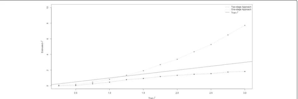
Figure 1 shows the estimated between-study varianceτˆ2 from both the two-stage (dashed line) and the one-stage (dotted line) approaches versus the true between-study variance,τ2(solid line). As the trueτ2increased, the esti-matedτˆ2from both approaches also increased. Compared with the estimatedτˆ2from a two-stage model, theτˆ2from the one-stage model increased more rapidly. The two-stage model always underestimatedτˆ2. On the other hand, the one-stage approach very slightly underestimated τˆ2 when the trueτ2was small, and it overestimatedτˆ2when the trueτ2was larger than 1.3.
Figure 2 shows the conventional I2 from the two-stage model (dashed line) and the simulation-based I2 from one-stage model (dotted line) versus the true between-study variance τ2. Both measures increased, then leveled off as the true between-study variance increased.
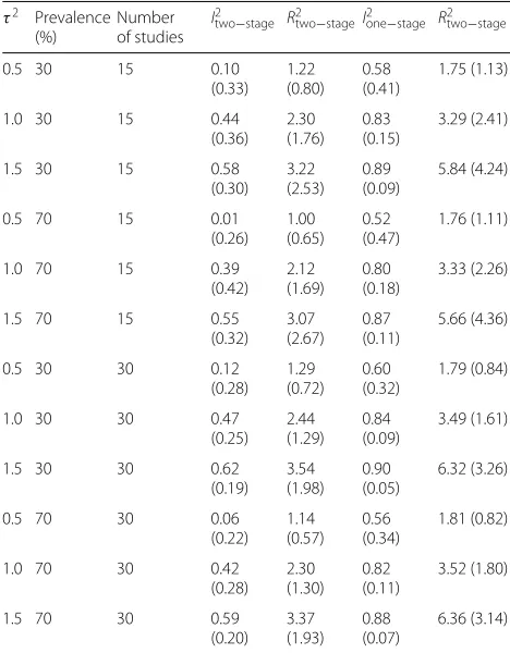
Table 2 presents the median value and IQR of the ˆI2 andRˆ2across 1000 datasets from the two-stage and one-stage models for different combinations of data generation parameter values. The median estimatedI2andR2from
Fig. 2Trueτ2versus estimatedI2. The estimatedI2from a conventional two-stage model and a simulation-based one-stage model are compared with the true between-study variance. The dashed line and dotted line represented the estimatedI2from the two-stage and one-stage models based on its median value across 1000 datasets
both the two-stage and one-stage model increased as the true between-study variance increased.ˆItwo2 −stageand ˆ
Ione2 −stage were very similar for N = 15 and N = 30.
However, the R2 statistic from both approaches slightly increased as the number of studies increased. Varying the
Table 2Median (IQR) of heterogeneity metrics for the treatment
effect when no effect modification was presenta
τ2 Prevalence (%)
Number of studies
I2two−stage R2two−stageI2one−stage R2two−stage
0.5 30 15 0.10
(0.33) 1.22 (0.80)
0.58 (0.41)
1.75 (1.13)
1.0 30 15 0.44
(0.36) 2.30 (1.76)
0.83 (0.15)
3.29 (2.41)
1.5 30 15 0.58
(0.30) 3.22 (2.53)
0.89 (0.09)
5.84 (4.24)
0.5 70 15 0.01
(0.26) 1.00 (0.65)
0.52 (0.47)
1.76 (1.11)
1.0 70 15 0.39
(0.42) 2.12 (1.69)
0.80 (0.18)
3.33 (2.26)
1.5 70 15 0.55
(0.32) 3.07 (2.67)
0.87 (0.11)
5.66 (4.36)
0.5 30 30 0.12
(0.28) 1.29 (0.72)
0.60 (0.32)
1.79 (0.84)
1.0 30 30 0.47
(0.25) 2.44 (1.29)
0.84 (0.09)
3.49 (1.61)
1.5 30 30 0.62
(0.19) 3.54 (1.98)
0.90 (0.05)
6.32 (3.26)
0.5 70 30 0.06
(0.22) 1.14 (0.57)
0.56 (0.34)
1.81 (0.82)
1.0 70 30 0.42
(0.28) 2.30 (1.30)
0.82 (0.11)
3.52 (1.80)
1.5 70 30 0.59
(0.20) 3.37 (1.93)
0.88 (0.07)
6.36 (3.14)
aPlease note thatI2is presented here as a proportion varying from 0 to 1, rather than as a percentage
prevalence from 30 to 70% did not affect the estimates of I2andR2via two- and one-stage models.
Furthermore, τˆ2 from the two- and one-stage approaches were similar for different prevalence and number of studies (Additional file 1: Table S1).
With effect modification
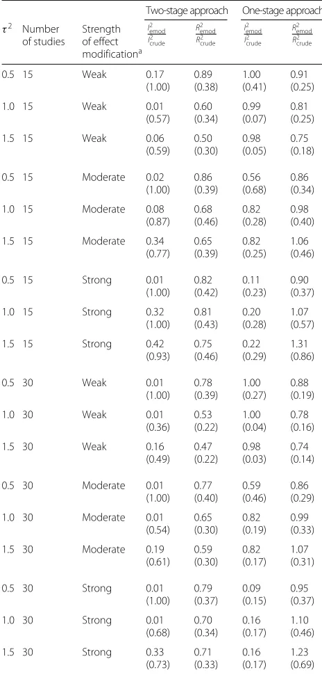
Table 3 presents the median value and IQR of the ratio ofI2andR2from a model that ignored the effect mod-ifier to one that included the effect modmod-ifier and an interaction term between it and the treatment status across 1000 datasets from the two-stage and one-stage approaches with prevalence = 30%. Any measure of heterogeneity should be sensitive to changes in hetero-geneity. If we did not account for effect modification when it existed, then heterogeneity might arise due to this effect modification [24]. Hence, if the ratio esti-mators reported in the Table 3 are less than 1, they indicate good sensitivity of the measure to changing heterogeneity.
Table 3Sensitivity of heterogeneity measures to accounting for effect modification when prevalence of the outcome was 30%
Two-stage approach One-stage approach τ2 Number
of studies Strength of effect modificationa I2 emod I2 crude R2 emod R2 crude I2 emod I2 crude R2 emod R2 crude
0.5 15 Weak 0.17
(1.00) 0.89 (0.38) 1.00 (0.41) 0.91 (0.25)
1.0 15 Weak 0.01
(0.57) 0.60 (0.34) 0.99 (0.07) 0.81 (0.25)
1.5 15 Weak 0.06
(0.59) 0.50 (0.30) 0.98 (0.05) 0.75 (0.18)
0.5 15 Moderate 0.02
(1.00) 0.86 (0.39) 0.56 (0.68) 0.86 (0.34)
1.0 15 Moderate 0.08
(0.87) 0.68 (0.46) 0.82 (0.28) 0.98 (0.40)
1.5 15 Moderate 0.34
(0.77) 0.65 (0.39) 0.82 (0.25) 1.06 (0.46)
0.5 15 Strong 0.01
(1.00) 0.82 (0.42) 0.11 (0.23) 0.90 (0.37)
1.0 15 Strong 0.32
(1.00) 0.81 (0.43) 0.20 (0.28) 1.07 (0.57)
1.5 15 Strong 0.42
(0.93) 0.75 (0.46) 0.22 (0.29) 1.31 (0.86)
0.5 30 Weak 0.01
(1.00) 0.78 (0.39) 1.00 (0.27) 0.88 (0.19)
1.0 30 Weak 0.01
(0.36) 0.53 (0.22) 1.00 (0.04) 0.78 (0.16)
1.5 30 Weak 0.16
(0.49) 0.47 (0.22) 0.98 (0.03) 0.74 (0.14)
0.5 30 Moderate 0.01
(1.00) 0.77 (0.40) 0.59 (0.46) 0.86 (0.29)
1.0 30 Moderate 0.01
(0.54) 0.65 (0.30) 0.82 (0.19) 0.99 (0.33)
1.5 30 Moderate 0.19
(0.61) 0.59 (0.30) 0.82 (0.17) 1.07 (0.31)
0.5 30 Strong 0.01
(1.00) 0.79 (0.37) 0.09 (0.15) 0.95 (0.37)
1.0 30 Strong 0.01
(0.68) 0.70 (0.34) 0.16 (0.17) 1.10 (0.46)
1.5 30 Strong 0.33
(0.73) 0.71 (0.33) 0.16 (0.17) 1.23 (0.69)
Median (IQR) was presented
We present the ratios of the measure estimated from a model that ignored the effect modifier to one that included the effect modifier and an interaction term between it and the treatment status
aEffect modification was classified as weak whenβ
w=1,βxw=1, as moderate
whenβw=1,βxw=3, and as strong whenβw=2,βxw=5
for one-stage approach decreased as the strength of effect modification became stronger (data not shown).
When the number of studies and prevalence were 30 and 30%, most of ratio estimators forItwo2 −stagewere equal to 0.01. This occurred because the estimated τtwo2 −stage
from the effect modification model was close to zero (Additional file 1: Table S3).
Furthermore, in Additional file 1: Table S3, the ratio esti-mators forτ2in the two-stage model were all less than or equal to 1. However, most of ratio estimators forτ2in the one-stage model were larger than 1.
Discussion
IPD-MA are the gold standard of meta-analytic approaches. While the primary objective of most IPD-MA is to estimate pooled treatment effects, quan-tifying inter-study heterogeneity of those effects is also an important goal. Most statisticians agree that a one-stage approach is the best and most flexible approach to use when analyzing data from IPD-MA. However, how best to quantify inter-study heterogene-ity in that case is unclear [3, 5, 12], and most IPD-MA of binary outcomes do not report any measure of heterogeneity [6].
In this work, we considered using usual measures of heterogeneity based on two-stage approaches, as well as novel approaches based on a one-stage model. We evalu-ated both two-stage and one-stage approaches via simula-tion studies. In the two-stage approach, we used the usual I2andR2statistics proposed by Higgins et al. to measure heterogeneity [5]. In the one-stage approach, we adapted a simulation-based ICC proposed by Goldstein et al. to estimate theI2, as well as considering theR2based on the one-stage model.
Our results demonstrated that when there was no effect modification, the estimatedτ2from the two-stage model was always underestimated. When using a one-stage approach, the estimated τ2 was underestimated when the trueτ2was small, but overestimated when the trueτ2was large. Correspondingly, we may assume that the estimatedI2from the two-stage model was underes-timated, whereas the simulation-basedI2in the one-stage model was underestimated when inter-study heterogene-ity was small and overestimated when it was large. Both the two-stageI2and one-stageI2increased as the trueτ2 increased.
using the simulation-basedI2based on one-stage model is preferable.
Differences between measures of heterogeneity in the two-stage and one-stage approaches might be due to real differences in the methods, or because slightly differ-ent models were used. In the one-stage approach, we only considered models that fit a random intercept and slope, while the two-stage approaches fit just a random slope. However, these are the approaches most commonly used [6].
Strengths of the work
We have proposed a simulation-based I2to use in one-stage IPD-MA of binary outcomes. We have shown that this I2 satisfies the conditions proposed by Higgins et al., for any measures quantifying heterogeneity, i.e., (i) the measurement function should monotonically increase with increasing between-study varianceτ2and (ii) not be affected by the number of studies N [5]. Moreover, we have shown that the simnulation-basedI2is sensitive to changes in heterogeneity.
When the outcome is binary, the within-study vari-ance varies across the studies as between-study varivari-ance increases [7]. As a result, the assumption of equal esti-mated sampling variances across all studies, as in Higgins and Thompson’s paper [5], does not hold, and Higgins’s I2 may be biased. For that reason, we would expect the simulation-basedI2based on the one-stage approach to have better performance than the conventionalI2based on the two-stage approach.
Using a heterogeneity measure based on the one-stage model is also advantageous, because the one-one-stage approach allows investigation of patient- and study-level covariates, and the treatment effect can be adjusted for covariates at the participant- or study-level [18]. More-over, the one-stage model allows MA of dose-response curves (e.g., allowing non-linearity), improves power for interactions [25, 26], and allows better control of effect modification by patient- and study-level covariates than the two-stage approach [3, 17, 27].
While we investigated its performance for binary out-comes, using the ICC as anI2for continuous outcomes in the context of a mixed model would be possible, though to our knowledge has not been used like this.
Limitations
There are several limitations in this work. We only con-sidered the ICC estimator proposed by Goldstein to esti-mate the I2 in one-stage IPD-MA of binary outcomes. However, there are several other measures that have been proposed as estimators of the ICC for binary data [14, 21, 22]. Wu et al. discussed five different methods to estimate the ICC with binary outcomes: an analysis of variance (ANOVA) estimator, the Fleiss-Cuzick estimator,
the Pearson estimator, an estimator based on general-ized estimating equations (GEE), and an estimator from the random intercept logistic model [20]. These could be adapted to estimateI2in one-stage IPD-MA. On the other hand, the measure we have proposed is easy to estimate.
Moreover, GLMMs estimated via adaptive quadrature sometimes do not converge in the one-stage model [19]. Indeed, we observed a sometimes important rate of non-convergence when the strength of effect modification was strong and the prevalence was high. Other estimation approaches such as penalized quasi-likelihood (PQL) or Bayesian multilevel models might be interesting to explore [28, 29]. While convergence of PQL is more likely, esti-mates can be biased with few subjects per cluster, low event rates, or high inter-cluster variability [7, 29, 30].
For the two-stage approaches, we estimatedτ2via the method of moments estimator of DerSimonian and Laird, despite more recent evidence suggesting that the Paule and Mandel estimator is preferred [31].
Finally, we invsestigated a finite number of data gener-ation parameters. In particular, we considered datasets of 15 or 30 studies, whereas it may have been interesting to consider fewer (e.g., 5).
Conclusion
When a one-stage approach for IDP-MA of binary out-comes is preferred, heterogeneity should be quantified via the model estimated. In that case, we have proposed a simulation-basedI2that performs as well or better than the conventionalI2based on a two-stage approach. TheR2 based on the one-stage model also performed adequately but is more difficult to interpret.
Additional file
Additional file 1: Table S1.The Median (IQR) of the estimatedτ2when
no effect modification was present.Table S2.Sensitivity of heterogeneity measures to accounting for effect modification when prevalence of the outcome was 70%. Median (IQR) was presented.Table S3.Sensitivity of
heterogeneity measures
τ2 emod τ2
crude
to accounting for effect modification.
Median (IQR) was presented. (PDF 145 kb)
Abbreviations
AD-MA: Aggregate data meta-analysis; ANOVA: Analysis of variance; GEE: Generalized estimating equation; GLMM: Generalized linear mixed model; ICC: Intraclass correlation coefficient; IPD-MA: Individual participant data meta-analysis; IQR: Interquartile range; MA: Meta-analysis; PQL: Penalized quasi-likelihood
Acknowledgements
We thanks the reviewers for their suggestions. A research grant from the Canadian Insitutes of Health Research (CIHR) supporterd this research. Andrea Benedetti is supported by the Fonds de recherche de Québec Santé.
Funding
Availability of data and materials
Rcode for dataset generation is avaliable by request.
Authors’ contributions
AB gave the original idea to conduct this research work. BC implemented this research work under the guidance of AB. Both authors read and approved the final manuscript.
Ethics approval and consent to participate Not applicable.
Consent for publication Not applicable.
Competing interests
The authors declare that they have no competing interests.
Publisher’s Note
Springer Nature remains neutral with regard to jurisdictional claims in published maps and institutional affiliations.
Received: 9 November 2016 Accepted: 17 November 2017
References
1. Lyman GH, Kuderer NM. The strengths and limitations of meta-analyses based on aggregate data. BMC Med Res Methodol. 2005;5(14):14–14. 2. What Is Meta-analysis? http://www.bandolier.org.uk/painres/download/
whatis/Meta-An.pdf. Accessed 5 Mar 2016.
3. Riley RD, Lambert PC, Abo-Zaid G. Meta-analysis of individual participant data: rationale, conduct, and reporting. BMJ. 2010;340:521–5.
4. Rücker G, Schwarzer G, Carpenter JR, Schumacher M. Undue reliance on i2 in assessing heterogeneity may mislead. BMC Med Res Methodol. 2008;8(1):79.
5. Higgins JPT, Thompson SG. Quantifying heterogeneity in a meta-analysis. Stat Med. 2002;21(11):1539–58.
6. Thomas D, Radji S, Benedetti A. Systematic review of methods for individual patient data meta- analysis with binary outcomes. BMC Med Res Methodol. 2014;14(1):79.
7. Zhou Y, Dendukuri N. Statistics for quantifying heterogeneity in univariate and bivariate meta-analyses of binary data: the case of meta-analyses of diagnostic accuracy. Stat Med. 2014;33(16):2701–17. 8. DerSimonian R, Laird N. Meta-analysis in clinical trials. Control Clin Trials.
1986;7(3):177–88.
9. Whitehead A, Whitehead J. A general parametric approach to the meta-analysis of randomized clinical trials. Stat Med. 1991;10(11):1665–77. 10. Biggerstaff BJ, Jackson D. The exact distribution of Cochran’s
heterogeneity statistic in one-way random effects meta-analysis. Stat Med. 2008;27(29):6093–110.
11. Jackson D, White IR, Riley RD. Quantifying the impact of between-study heterogeneity in multivariate meta-analyses. Stat Med. 2012;31(29): 3805–20.
12. Debray TPA, Moons KGM, Abo-Zaid GMA, Koffijberg H, Riley RD. Individual participant data meta-analysis for a binary outcome: one-stage or two-stage? pone. 2013;8(4):60650.
13. Jackson D, Bowden R, Baker J. How does the DerSimonian and Laird procedure for random effects meta-analysis compare with its more efficient but harder to compute counterparts? J Stat Plan Infer. 2010;48(4): 961.
14. Ridout MS, Demetrio CGB, Firth D. Estimating intraclass correlation for binary data. Biometrics. 1999;55(1):137–48.
15. Yelland LN, Salter AB, Ryan P, Laurence CO. Adjusted intraclass correlation coefficients for binary data: methods and estimates from a cluster-randomized trial in primary care. Clin Trials. 2011;8(1):48–58. 16. Thomson A, Hayes R, Cousens S. Measures of between-cluster variability
in cluster randomized trials with binary outcomes. Stat Med. 2009;28(12): 1739–51.
17. Riley RD, Lambert PC, Staessen JA, Wang J, Gueyffier F, Thijs L, Boutitie F. Meta-analysis of continuous outcomes combining individual patient data and aggregate data. Stat Med. 2008;27(11):1870–93.
18. Higgins JPT, Whitehead A, Turner RM, Omar RZ, Thompson SG. Meta-analysis of continuous outcome data from individual patients. Stat Med. 2001;20(15):2219–41.
19. Diggle P. Analysis of longitudinal data. Oxford: Oxford University Press; 2002.
20. Wu S, Crespi CM, Wong WK. Comparison of methods for estimating the intraclass correlation coefficient for binary responses in cancer prevention cluster randomized trials. Contemp Clin Trials. 2012;33(5):869–80. 21. Browne WJ, Subramanian SV, Jones K, Goldstein H. Variance partitioning
in multilevel logistic models that exhibit overdispersion. J R Stat Soc Ser A (Stat Soc). 2005;168(3):599–613.
22. Goldstein H, Browne W, Rasbash J. Partitioning variation in multilevel models. Underst Stat. 2002;1(4):223.
23. The R project for statistical computing. https://www.r-project.org/. Accessed 5 Jan 2016.
24. Gentles SJ, Stacey D, Bennett C, Alshurafa M, Walter SD. Factors explaining the heterogeneity of effects of patient decision aids on knowledge of outcome probabilities: a systematic review sub-analysis. Syst Rev. 2013;2:95.
25. Lambert PC, Sutton AJ, Abrams KR, Jones DR. A comparison of summary patient-level covariates in meta-regression with individual patient data meta-analysis. J Clin Epidemiol. 2002;55(1):86–94.
26. Schmid CH, Stark PC, Berlin JA, Landais P, Lau J. Meta-regression detected associations between heterogeneous treatment effects and study-level, but not patient-level, factors. J Clin Epidemiol. 2004;57(7): 683–97.
27. Riley RD. Commentary: like it and lump it? Meta-analysis using individual participant data. Int J Epidemiol. 2010;39(5):1359–61.
28. Brewlow NE, Clayton DG. Approximate inference in generalized linear mixed models. J Am Stat Assoc. 1993;88:421.
29. Jang W, Lim J. A numerical study of PQL estimation biases in generalized linear mixed models under heterogeneity of random effects. Commun Stat Simul Comput. 2009;38:692–702.
30. Lin X, Breslow NE. Bias correction in generalized linear mixed models with multiple components of dispersion. J Am Stat Assoc. 1996;91(435):1007. 31. Veroniki AA, Jackson D, Viechtbauer W, Bender R, Bowden J, Knapp G,
Kuss O, Higgins JP, Langan D, Salanti G. Methods to estimate the between-study variance and its uncertainty in meta-analysis. Res Synth Meth. 2016;7(1):55–79.
• We accept pre-submission inquiries
• Our selector tool helps you to find the most relevant journal
• We provide round the clock customer support
• Convenient online submission
• Thorough peer review
• Inclusion in PubMed and all major indexing services
• Maximum visibility for your research
Submit your manuscript at www.biomedcentral.com/submit