Adding Constraints to Bayesian Inverse Problems

The Thirty-Third AAAI Conference on Artificial Intelligence (AAAI-19)

Adding Constraints to Bayesian Inverse Problems

Jiacheng Wu

Berkeley, CA, 94706

Jian-Xun Wang

Notre Dame, IN, 46556

Shawn C. Shadden

Abstract

Using observation data to estimate unknown parameters in computational models is broadly important. This task is of-ten challenging because solutions are non-unique due to the complexity of the model and limited observation data. How-ever, the parameters or states of the model are often known to satisfy additional constraints beyond the model. Thus, we propose an approach to improve parameter estimation in such inverse problems by incorporating constraints in a Bayesian inference framework. Constraints are imposed by construct-ing a likelihood function based on fitness of the solution to the constraints. The posterior distribution of the parameters conditioned on (1) the observed data and (2) satisfaction of the constraints is obtained, and the estimate of the parame-ters is given by the maximum a posteriori estimation or pos-terior mean. Both equality and inequality constraints can be considered by this framework, and the strictness of the con-straints can be controlled by constraint uncertainty denot-ing a confidence on its correctness. Furthermore, we extend this framework to an approximate Bayesian inference frame-work in terms of the ensemble Kalman filter method, where the constraint is imposed by re-weighing the ensemble mem-bers based on the likelihood function. A synthetic model is presented to demonstrate the effectiveness of the proposed method and in both the exact Bayesian inference and ensem-ble Kalman filter scenarios, numerical simulations show that imposing constraints using the method presented improves identification of the true parameter solution among multiple local minima.

1

Introduction

Computational models are pervasively used in wide-ranging engineering applications. Recent advances in computer plat-forms and numerical methods have enabled models to be increasingly sophisticated and comprehensive.With greater model complexity comes greater challenge to determine model parameters (including initial/boundary conditions), which are often unknown or uncertain. To address this challenge, one typically solves aninverse problem by us-ing observational data to specify model parameters so that the model output matches the observational data. Many in-version techniques have been developed and used by dif-ferent communities. These methods can be roughly cat-Copyright c⃝2019, Association for the Advancement of Artificial Intelligence (www.aaai.org). All rights reserved.

egorized into two classes: variational and statistical ap-proaches (Asch, Bocquet, and Nodet 2016). The varia-tional approach aims to minimize a specific cost function based on classical optimization theory and calculus of vari-ations (Smedstad and O’Brien 1991), while the statistical approach aims to evaluate or maximize posterior functions based on statistics and Bayesian theory (Cotter et al. 2009).

Because of its robustness and capability for uncertainty quantification, Bayesian inversion techniques are widely used for hidden state and parameter estimation for many physical systems (Iglesias, Lin, and Stuart 2014; Wang et al. 2017; Wang and Xiao 2016; Li et al. 2017). In the Bayesian framework, both the hidden state/parameters (prior) and observable quantities (likelihood) are described as random variables with statistical distributions. The Bayesian esti-mation aims to calculate the posterior distributions of the inferred quantities from the prior and likelihood based on Bayes theorem. Directly computing the posterior distribu-tion based on the prior and likelihood funcdistribu-tions is referred to as the exact Bayesian approach. In general, the posterior is obtained by sampling the prior and likelihood distributions based on efficient Monte Carlo sampling such as the Markov chain Monte Carlo (MCMC) method. However, since MCMC requires an enormous amount of samples, which is computationally infeasible when the likelihood calcula-tion involves expensive model evaluacalcula-tions, many approxi-mate Bayesian inversion approaches have been developed, such as the extended Kalman filter (EKF) (Haykin 2004), unscented Kalman filter (UKF) (Wan and Van Der Merwe 2000), ensemble Kalman filter (EnKF) (Evensen 2003), and sequential Monte Carlo (SMC) method (Del Moral, Doucet, and Jasra 2006).

help regularize the inversion results to consistent ranges and relieve ill-posedness. Fortunately, for many physical sys-tems, constraints on the state and parameters are available based on existed knowledge (He and Xiu 2016). Nonethe-less, most existing Bayesian methods do not take constraints into account (Shao, Huang, and Lee 2010).

Initial progress has been made to incorporate constraints into certain Bayesian filters. For example, Simon et al. (Si-mon and Chia 2002) considered equality constraints in the standard Kalman filter by projecting the Kalman updated solution onto the state constraint surface. Shao et al. (Shao, Huang, and Lee 2010) developed a constrained sequential Monte Carlo algorithm based on acceptance/rejection and an optimization strategy. Most recently, Gardner et al. (Gard-ner et al. 2014) also considered inequality constraints in the context of Bayesian optimization. However, the existing ap-proaches to incorporate constraints have been developed for each specific Bayesian filter, and most of them are based on a linearized form of the constraints, which is limiting when constraint functions are complicated and highly nonlinear. Moreover, in many complex systems, the constraints are ap-proximations to reality and formulating the constraint in a deterministic way may neglect the uncertainties associated with constraint itself. In this work, we proposed a general approach to incorporate physics-based constraints into the Bayesian inversion framework, where uncertainty associated with the constraint itself can also been considered. More-over, this idea is also extended to an approximate Bayesian approach–the ensemble Kalman filter.

2

Methodology

A mathematical model of system defines aforward problem

that can be formulated as

x=F(θ), (1)

whereθ ∈ Rdθ are model parameters and x ∈ Rdx are the

states of the system. The forward operatorF is nominally assumed to describe a physical system, wherebyFtypically represents a suite of algebraic and/or differential equations. In most cases, the model parametersθare uncertain or un-known, and the state variables xare largely unobservable.

Therefore, the unknown parameters and hidden states need to be inferred from observationsy∈Rdy. These observations

indirectly and incompletely describe the state of the system, which can be formulated mathematically as

y=Hx+ϵ, (2)

where H is a projection operator projecting the full state to the observed space and ϵrepresents measurement error. The standard inverse problem deals with estimating the un-known parametersθ (or the hidden states x) based on the observationsy. In practice, approximate Bayesian inversion frameworks, such as Kalman filtering and Sequential Monte Carlo, are used for computational efficiency.

Constraints in Exact Bayesian Inference

Inverse problems are typically ill-posed because the obser-vational data is not sufficient to uniquely determine the un-known parameters. Thus, specification of additional con-straints can be useful to regularize the inverse problem.

Equality constraints can be defined with respect to the state variablesxas,

G(x) =[g₁₍x), g₂₍x)_{, ..., gdg}(x)]T =0, (3) where _gi(x), i = 1,2, ..., dg represent different equality con-straints. In many application, the constraint only approxi-mates reality. Thus, instead of directly imposing a hard con-straint, we assume that each constraint satisfies a zero-mean Gaussian distribution, expressed as

G(x)∼ N(0,Σc). (4) where theΣcis a covariance matrix used to control the strict-ness of each constraint. Sincexis intrinsically a function of θ, the constraints can alternatively be expressed in terms of the parameters

G(x) =G(F(θ))∼ N(0,Σc). (5) As such, these constraints on the parametersθcan be more naturally considered within the Bayesian framework by im-posing additional likelihood functions introduced by these nondeterministic constraints.

Without loss of generality, both the prior and likelihood are assumed Gaussian. Namely, the prior of the parameters θis defined by

p(θ) = _√ 1 (2π)dθ|Σ_θ|

exp

(

−1

2(θ− ˆ

θ)TΣ−1_θ (θ−_θˆ₎)_{, (6)}

where_θˆ_andΣ

θare the prior mean and covariance, which are based on existing knowledge or preliminary estimation. The observation data errors are also assumed to follow a zero-mean Gaussian distribution, i.e.,ϵ∈N(0,Σ_l), thus the

likeli-hood of the observed data set onyis, p(D|θ) =_√ 1

(2π)dy|Σ_l| exp

(

−1

2(y−HF(θ))

T_Σ−1

l (y−HF(θ)) )

.

(7) The covariance matrixΣ_lis obtained by estimating the

sam-ple variance of the observed data setsD. The constraints are imposed by considering the following likelihood function,

p(G(x) =0|θ)

=_√ 1

(2π)dg|Σc| exp

(

−1

2G(F(θ))

T_Σ−1

c G(F(θ)) )

. (8)

The likelihood of the constraints defines a fitness of a spe-cific value ofθbased on the satisfaction of the constraints. By introducing this Gaussian-type likelihood function, we enable a “soft” enforcement of the constraints. The strictness of the constraint can be controlled by the diagonal variance matrixΣc,

Σc=diag{σ2_c,1, σ2_c,2, ..., σ2_c,dg}. (9) where the variance _σi represent a confidence on the accu-racy of the constraint. Smaller_σc,icorresponds to a stricter constraint.

Inequality constraints can be converted to equivalent equality constraints. For example, a scalar inequality con-straintg(x)≤0can be expressed as

and thus the corresponding likelihood can be expressed as

p(g(x)≤0|θ) =√1

2πσ_c2

exp

(

− 1

2σ2_c [max (0, g(x))]

2

) . (11)

Imposing constraints through a likelihood function can also be extended to disjunctive constraints. For example, consider a constraint of the formg₁₍x) = 0∨g₂₍x) = 0. By

the union rule of probability

p(g₁₍x) = 0∨g₂₍x) = 0|θ)

=p(g₁₍x) = 0|θ) +p(g₂₍x) = 0|θ)−p(g₁₍x) = 0∧g₂₍x) = 0|θ)

=√ 1

2πσ_c,2₁

exp

⎛

⎝−

g₁₍F(θ))2 2σ2_c,1

⎞

⎠+

1

√

2πσ_c,2₂

exp

⎛

⎝−

g₂₍F(θ))2 2σ2_c,2

⎞

⎠

−√ 1

(2π)2|Σc| exp

⎛

⎝−

1 2

[ g₁₍F(θ))

g₂₍F(θ))

]T

Σ−1_c

[ g₁₍F(θ))

g₂₍F(θ))

]⎞

⎠ , (12)

whereΣcagain defines the covariance matrix of constraints. With the prior distribution, likelihood of the data, and likelihood of the constraints now defined, the posterior prob-ability distribution conditioned on the observed dataDand the constraintsG(x)can be defined as

p(θ|D, G(x) =0) = p(D|θ)p(G(x) =0|θ)p(θ)

p(D, G(x) =0)

∝p(D|θ)p(G(x) =0|θ)p(θ). (13)

Since the posterior distribution cannot be solved analytically in general, it is commonly evaluated based on MCMC sam-pling.

Constraints in Approximate Bayesian Inference

The direct Bayesian inference based on MCMC sampling is usually intractable when the likelihood calculation in-volves a computationally expensive model; instead approx-imate Bayesian approaches are commonly used to provide a more computationally tractable solution. The EnKF is one such method, which is a variant of the standard Kalman fil-ter where the covariance matrix is replaced by Monte Carlo samples.

For EnKF, we combine the original hidden statesxand the unknown parametersθinto a new augmented state

z=[θT, xT]T , (14) which will be updated during the filtering process accord-ing to the observed dataD. The initial ensemble is first ob-tained by sampling the prior distributionp(θ)and evaluating

the model at each ensemble member

{

ˆ

z(j) }J

j=1 =

{_[

ˆ

θ(j); ˆx(j) ]T}J

j=1 =

{_[

ˆ

θ(j);F (

ˆ

θ(j) )]T}J

j=1

,

(15) whereJis the number of ensemble members. The probabil-ity associated with each ensemble member is initially set to be uniform

wj,p(z= ˆz(j)) = 1

J, j= 1,2, ..., J . (16)

Then the expectation and covariance matrix of the state vari-ables are estimated from the ensemble as

E(ˆz) =

J ∑

j=1

wjzˆ(j), (17)

C(ˆz) =

J ∑

j=1

wj(ˆz(j)−E(ˆz))(ˆz(j)−E(ˆz))T. (18)

If the observed data follows a normal distributionN(¯y,Σ_l),

the prior ensemble can be updated by the observed dataD

according to the Kalman update

z(j)= ˆz(j)+C(ˆz)HT(HC(ˆz)HT+ Σ_l)−1(¯y−Hz(j)), j= 1,2, ..., J . (19)

The posterior ensemble{ z(j)}J

j=1represents a sampling for

the posterior probability distributionp(z|D), with the proba-bility associated with each ensemble member equal to

p(z(j)|D) =_{wj ,} ∀j= 1,2, ..., J . (20)

Now we consider inclusion of constraints. The likelihood of the constraintG(x) =0to be satisfied conditioned on each

member of the posterior ensemble can be computed as

Lg(j),p (

G(x) =0|z(j) )

=√ 1

(2π)dg|Σc| exp

(

−1

2G

( x(j)

)T

Σ−1_c G (

x(j) ))

.

(21) By Bayes theorem, the posterior probability density of each ensemble member conditioned on the observed dataDand

constraintsG(x) =0is given by

p (

z(j)|D, G(x) =0

)

= 1

Zp (

G(x) =0, z(j)|D

)

= 1

Zp (

G(x) =0|z(j) )

p (

z(j)|D

)

= 1

Zwj Lg

(j) ₍₂₂₎

whereZis the normalization constant defined as

Z=

J ∑

j=1

p (

G(x) =0|x(j) )

p (

x(j)|D

)

=

J ∑

j=1

wj Lg(j). (23)

The empirical distribution for p(z|D, G(x) =0) can be

de-scribed by the posterior ensemble{ z(j)}J

j=1, and the

associ-ated probability mass

p (

z=z(j)|D, G(x) =0

)

= wj Lg (j)

∑J

p=1wj Lg(p)

, ∀j= 1,2, ..., J,

(24) for each ensemble member. We here re-define the new weights for each ensemble members as

w′_j, wj Lg

(j)

∑J

p=1wj Lg(p)

. (25)

thatG(x) =0according to

¯

z=E(z|D, G(x) =0) =

J ∑

j=1

p (

z=z(j)|D, G(x) =0

) z(j)

=

J ∑

j=1

w_{j z}′ (j). (26)

Then the estimation of the unknown parameters _θ¯_{can be}

extracted from the estimation of the full augmented state. Also, the covariance of the parameter θ with respect to p(z|D, G(x) =0)can be computed as

Σ_θ=

J ∑

i=1

(

θ(j)−_θ¯)_diag{ w′_j}J

j=1

(

θ(j)−_θ¯)T _{. (27)}

The new prior ensemble for the next iteration step is ob-tained by sampling the following normal distribution

ˆ

θ(j)∼N( ¯θ,Σ_θ), j= 1,2, ..., J , (28) to maximize the next step prior entropy (Penfield Jr 2010) while keeping the mean and covariance the same as the pre-vious posterior distribution. The iterative process continues until a stopping criterion is satisfied or the maximum itera-tion number is reached.

3

Results and Discussion

Model Test Problem

To verify the effectiveness of the constrained Bayesian infer-ence framework described above, a simple test case is pre-sented here. The forward model mapping from the parameter spaceΘ⊂R2to the state spaceX⊂R2is defined as

[ x₁ x₂ ]

=F(θ) =

[

exp(−(θ_{1 + 1)}2−(θ_{2 + 1)}2)

exp(−(θ₁−1)2−(θ₂−1)2)

]

. (29) The projection matrix mapping from state space to output is given by

H= [−1.5,−1.0], (30)

and thus the reconstructed output is

HF(θ) =−1.5 exp(−(θ_{1 + 1)}2−(θ_{2 + 1)}2)

−1.0 exp(−(θ₁−1)2−(θ₂−1)2), (31) whereHF(θ)∈R1. We consider the following constraint:

G(x) =−0.25 logx_{1 + 0}.25 logx₂−2 = 0, (32)

which can be equivalently written in terms ofθ,

G(F(θ)) =θ_{1 +}θ₂−2 = 0. (33)

We assume the observed data follow the normal distribution N(¯y,Σ_l)where the meany¯=−1.0and the covariance matrix

Σ_lis chosen based on the uncertainty associated with data.

This model is chosen to create a simple scenario with mul-tiple local minimums. Namely, regardless of the prior infor-mation and constraints, we seek the model parameters that minimize the difference between the observed output and re-constructed output, quantified by the cost function

I(θ) =∥¯y−HF(θ)∥2

=(1.5 exp(−(θ_{1 + 1)}2−(θ_{2 + 1)}2)

+1.0 exp(−(θ₁−1)2−(θ₂−1)2)−1.0)2 . (34)

θ1

-3 -2 -1 0 1 2 3

θ2

-3 -2 -1 0 1 2 3

0.1

0.1

0.1 0.1

0.1

0.1

0.2 0.2

0.2 0.2

0.2

0.2

0.3

0.3

0.3 0.3

0.3

0.3

0.4 0.4

0.4

0.4

0.4

0.4

0.4

0.5

0.5

0.5 0.5

0.5

0.5

0.5 0.6 0.6

0.6 0.6

0.6

0.6

0.6 0.7 0.7

0.7

0.7

0.7

0.7

0.7

0.8 0.8

0.8

0.8

0.8

0.8

0.8 0.9

0.9

0.9

0.9 0.9

0.9

0.9

0.9

Cost function: I(θ)

local minimums

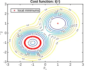
Figure 1: Contour plot of the cost functionI(θ)with respect

to parametersθ= [θ₁, θ_2]The red “+” denote the local min-ima of the cost function.

θ1

-5 0 5

θ2

-8 -6 -4 -2 0 2 4 6

8 (a)

θ1

-5 0 5

θ2

-8 -6 -4 -2 0 2 4 6

8 (b)

θ1

-5 0 5

θ2

-8 -6 -4 -2 0 2 4 6

8 (c)

θ1

-5 0 5

θ2

-8 -6 -4 -2 0 2 4 6

8 (d)

Figure 2: (a) Sampling of the prior distribution; (b) Sam-ple + data likelihood p(D|θ); (c) Sample + constraint

like-lihood p(G(x) = 0|θ); (d) Sample + posterior distribution

p(θ|D, G(x) =0)

which has minimums at (a)θ∗= (1,1); and (b)θon the circle defined by

(θ_{1 + 1)}2+ (θ_{2 + 1)}2= log 1.5. (35)

The contour plot of the cost function and the local mini-mums are visualized in Figure 1. Here we assumeθ∗= (1,1)

is the true value of the parameterθ, and the constraint (33) will help to eliminate convergence to other local minima.

The situation of multiple local minima is a common chal-lenge in solving inverse problems, because the observed out-put information is usually not enough to uniquely determine the unknown parameters. We show below that imposing con-straints can help the solution to converge to the true value.

Exact Bayesian Inference

The prior distribution (6) is first sampled withJ= 5000

sam-ples. The mean and the covariance matrix are set to

ˆ

θ=

[

0

0

] , Σ_θ=

[

3 0

0 3

]

. (36)

θ1 θ2 x1 x2 y

True values 1 1 0 1 -1

No constraint -0.0448 -0.0722 0.1698 0.1063 -0.3610

With constraint: EXP 0.9926 0.9449 0.0004 0.9969 -0.9976

With constraint: MAP 0.9845 0.9698 0.0004 0.9988 -0.9994

Table 1: Parametersθ, statesx and output y estimated us-ing sample-based Bayesian inference with no constraint im-posed and with constraint imim-posed.

knowledge ofθ, and the large variance defined byΣ_θabove

denotes large uncertainty about the prior. Ideally if better prior knowledge exists, we can specify a better prior here, with more accurate mean and less uncertainty. After sam-pling the prior, the likelihood function of datap(D|θ)is

eval-uated at each individual sample point{ θ(j)}J

j=1. The

like-lihood of the data is plotted with respect to each sample in Figure 2(b). The value of the likelihood is indicated by the brightness of the sample. It can be clearly observed that the brightest regions coincide with the local minimums in Fig-ure 1, which shows the region of the highest likelihood of data . Similarly, we evaluate the likelihood function of the constraintp(G(x) =0|θ)at each sample, and the likelihood is

visualized in Figure 2(c). The region with the highest likeli-hood represents the form of the constraint in(θ₁, θ₂₎space, which isθ_{1 +}θ₂−2 = 0. The variance for the constraint is

set to beΣc= 0.5, which controls how strict the constraint is

enforced. Lastly, the posteriorp(θ|D, G(x) =0)is evaluated at

each samples, and the distribution of the sample along with the posterior weights are plotted in Figure 2(d). It is clearly observed that the location with the highest posterior density correspond to the intersection between the regions with high likelihood of data D and high likelihood of the constraint

satisfaction. This intersection region picks out the true value of the parameter θ. Computing the weighted sum of the parameter samples {

θ(j)}J

j=1 with respect to the posterior

weights yields the final estimation of the unknown parame-terθ∗

Exp= ∑J

j=1p

(

θ(j)|D, G(x) =0)θ(j) =∑J

j=1wj θ(j).Or

simply taking the sample θ(j) that maximize the posterior p(θ(j)|D, G(x) =0)yields the maximum a posteriori

estima-tion (MAP) of the unknown parameter, i.e.θ∗

MAP. Once the parameter is estimated, the estimated value of the state vari-ablesxand outputycan be computed by evaluating the for-ward modelF(θ∗). These estimated values are listed in Table

1 for the case of including and not including constraint. It can be seen from this table that imposing the constraint sig-nificantly increase the estimation accuracy in the case where multiple local minimums exist.

Approximate Bayesian Inference

No constraint imposed. Iterative ensemble Kalman fil-ter estimates the unknown model paramefil-tersθin a iterative manner. Since the cost functionI(θ)has multiple local

mini-mums, different initial guesses ofθwill converge to different

θ

1

-3 -2 -1 0 1 2 3

θ2

-3 -2 -1 0 1 2 3

0.1 0.1

0.1 0.1

0.1

0.1

0.2 0.2

0.2 0.2

0.2

0.2

0.3

0.3

0.3 0.3

0.3

0.3

0.4 0.4

0.4

0.4 0.4

0.4

0.4

0.5 0.5

0.5 0.5

0.5

0.5

0.5 0.6

0.6

0.6 0.6

0.6

0.6

0.6 0.7

0.7

0.7

0.7

0.7

0.7

0.7 0.8

0.8

0.8

0.8

0.8

0.8

0.8 0.9

0.9

0.9

0.9 0.9

0.9

0.9

0.9

Cost function: I(θ)

local minimums initial guesses converged values

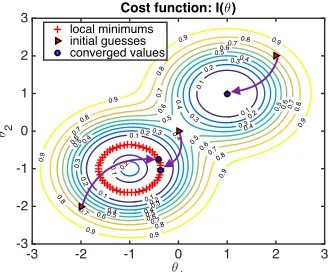
Figure 3: Different initial guesses of the unknown parameter θ(marked with red triangles) and their corresponding con-verged values after 1000 EnKF iteration steps (marked with blue circles), with no constraint imposed.

local minimums. We here define

Group I,{θ∗∈R2|θ∗= (1,1)} , (37) Group II,{θ∗∈R2|(θ∗1 + 1)2+ (θ∗2 + 1)2= log 1.5

} , (38) which represent two different local minimum regions. θ∗ represents the converged value of the parameter after ensem-ble Kalman filter iterations.

Here we simulated three different cases with different ini-tial guesses: (a)θ0 = (−2,−2); (b)θ0 = (0,0); (c)θ0 = (2,2).

The covariance matrix of the prior and the covariance of the data likelihood are given asΣ_θ= [1,0; 0,1]andΣ_l= 0.01. The results for the three different simulations are visualized in the parameter space ofθin Figure 3. It can be seen that the upper right initial guess at(2,2)converges to local minimum

Group I, and the other two initial guesses both converge to local minimum Group II. The convergence processes of the parameterθ for the three different initial guesses are plot-ted in Figure 4. It can be seen that all converge to the corre-sponding local minimum groups within about 400 iterations. The main difference is that while Case (c) converges to the local minimum(1,1), i.e., Group I, directly after a few

iter-ations, Case (a) and (b) converge toθ= (−1,−1)first, which

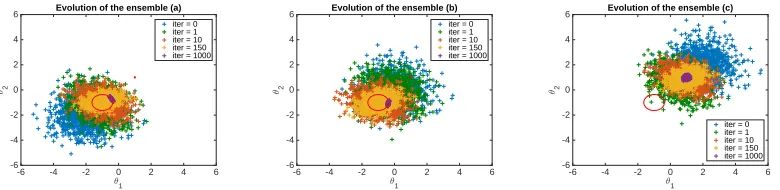
is the center of the local minimum circle of Group II, and then shift to a local minimum on the circle of Group II at around the 200th iteration (indicated by the “jump”). The reason behind this is that we use the mean of the ensemble of each step as the estimated parameter value. When the en-semble converges to the local neighborhood of Group II, the mean of the ensemble will generally be the center of the lo-cal minimum circle because the high likely ensemble mem-bers are roughly symmetrically distributed around the cen-ter(−1,−1). The mean of the ensemble will gradually shift to certain points on the circle based on the distribution of the ensemble members. The evolution of the ensemble for different initial guesses is shown in Figure 5. It can be seen that the variance of the ensemble gradually decrease until all ensemble members collapse to the corresponding local minimum.

iteration number

200 400 600 800 1000

θ

-2 -1.8 -1.6 -1.4 -1.2 -1 -0.8 -0.6 -0.4

-0.2 Convergence of the parameter θ (a)

θ1

θ2

iteration number

200 400 600 800 1000

θ

-1.4 -1.2 -1 -0.8 -0.6 -0.4 -0.2

0 Convergence of the parameter θ (b)

θ1

θ2

iteration number

200 400 600 800 1000

θ

0.6 0.8 1 1.2 1.4 1.6 1.8

2 Convergence of the parameter θ (c)

θ1 θ2

Figure 4: Results for the convergence of the parameterθwith no constraint imposed. (a) Initial guessθ0 = (−2,−2); (b) initial

guessθ0 = (0,0); (c) initial guessθ0 = (2,2).

θ1

-6 -4 -2 0 2 4 6

θ2

-6 -4 -2 0 2 4

6 Evolution of the ensemble (a)

iter = 0 iter = 1 iter = 10 iter = 150 iter = 1000

θ1

-6 -4 -2 0 2 4 6

θ2

-6 -4 -2 0 2 4

6 Evolution of the ensemble (b)

iter = 0 iter = 1 iter = 10 iter = 150 iter = 1000

θ1

-6 -4 -2 0 2 4 6

θ2

-6 -4 -2 0 2 4

6 Evolution of the ensemble (c)

iter = 0 iter = 1 iter = 10 iter = 150 iter = 1000

Figure 5: Evolution of the ensemble of the parameterθwith no constraint imposed. The points on the red circle centered at (-1,-1) and the red point at (1,1) denote the local minimums of the cost functionI(θ). (a) Initial guessθ0 = (−2,−2); (b) initial guessθ0 = (0,0); (c) initial guessθ0 = (2,2).

guesses are summarized here,

θ0= (−2,−2)→θ∗= (−0.4080,−0.7598)∈Group II, θ0= (0,0)→θ∗= (−0.3654,−1.0421)∈Group II, θ0= (2,2)→θ∗= (0.9998,0.9812)∈Group I.

The reconstructed outputs HF(θ∗) for the above cases all

converge to the target valuey¯=−1within 1000 EnKf

itera-tions. However, with no constraint is imposed, the estimate of the parameter θwill converge to the closer local mmum group based on where the initial guesses are. The ini-tial guess in the middle(0,0)converges to the local minimum

Group II because Group II contains more local minimums than Group I, and therefore the the solution is more likely to converge to Group II when initial guess is in the middle. More broadly, there is no guarantee that the estimate of the parameter will converge to the the true parameter value(1,1).

With constraint imposed For the local minimums in Group I and Group II, only the true parameter value (1,1)

satisfies the constraint. We test here whether imposing the constraint can help the convergence of the parameter esti-mation to the true value.

Three cases of different initial guesses are simulated with constraint imposed by re-weighing individual ensembles based on their likelihood of satisfying the constraint (see (26)). The covariances areΣ_θ= [1,0; 0,1]andΣ_l= 0.01, which

are kept the same as previous simulations. The covariance of the constraint used here isΣc= 2.0, which defines a certainty about the constraint. The simulation results are shown in Ta-ble 2 and visualized in Figure 6 (left). It can be seen that the solution converges to the true value(1,1)when starting from

(0,0)and(2,2), and the solution converges to the local

min-imum Group II when starting from(−2,−2). It is interesting to note that the middle initial point(0,0), which originally

converges to Group II, now is able to converge to the true value(1,1).

The reason that the solution starting from the lower left initial guess(−2,−2)cannot converges to the true value(1,1)

is because it is too far way from the true value and the vari-ance of the prior is not large enough to sample the parame-ter space near the true value(1,1). Therefore, even though the

constraint has been imposed, the solution cannot converge to the true value. To verify this, we simulated the three different starting locations with a larger prior varianceΣ_θ= [3,0; 0,3],

while the covariance of the data likelihoodΣ_l= 0.01and the

covariance of the the constraintΣc = 2.0are kept the same.

The simulation results are shown in Table 3 and visualized in Figure 6 (middle), demonstrating that all the three initial guesses lead to the true parameter value(1,1).

As a further test, we decreased the variance of the con-straintΣcto1.0to see how this influences the parameter

es-timation. The results in Table 4 and Figure 6 (right) demon-strate that (contrary to original conditions in the left panel) all three initial guesses converge to the true parameter value θ∗ = (1,1). Thus decreasing the variance of the constraint

can also improve convergence to the true parameter value in cases where the constraint is more certain.

Relation between Bayesian inference and

optimization

θ₁

-3 -2 -1 0 1 2 3

θ2 -3 -2 -1 0 1 2 3 0.1 0.1 0.1 0.1 0.1 0.1 0.2 0.2 0.2 0.2 0.2 0.2 0.3 0.3 0.3 0.3 0.3 0.3 0.4 0.4 0.4 0.4 0.4 0.4 0.4 0.5 0.5 0.5 0.5 0.5 0.5 0.5 0.6 0.6 0.6 0.6 0.6 0.6 0.6 0.7 0.7 0.7 0.7 0.7 0.7 0.7 0.8 0.8 0.8 0.8 0.8 0.8 0.8 0.9 0.9 0.9 0.9 0.9 0.9 0.9 0.9

Cost function: I(θ)

local minimums initial guesses converged values

θ₁

-3 -2 -1 0 1 2 3

θ2 -3 -2 -1 0 1 2 3 0.1 0.1 0.1 0.1 0.1 0.1 0.2 0.2 0.2 0.2 0.2 0.2 0.3 0.3 0.3 0.3 0.3 0.3 0.4 0.4 0.4 0.4 0.4 0.4 0.4 0.5 0.5 0.5 0.5 0.5 0.5 0.5 0.6 0.6 0.6 0.6 0.6 0.6 0.6 0.7 0.7 0.7 0.7 0.7 0.7 0.7 0.8 0.8 0.8 0.8 0.8 0.8 0.8 0.9 0.9 0.9 0.9 0.9 0.9 0.9 0.9 Cost function: I(θ) local minimums initial guesses converged values

θ₁

-3 -2 -1 0 1 2 3

θ2 -3 -2 -1 0 1 2 3 0.1 0.1 0.1 0.1 0.1 0.1 0.2 0.2 0.2 0.2 0.2 0.2 0.3 0.3 0.3 0.3 0.3 0.3 0.4 0.4 0.4 0.4 0.4 0.4 0.4 0.5 0.5 0.5 0.5 0.5 0.5 0.5 0.6 0.6 0.6 0.6 0.6 0.6 0.6 0.7 0.7 0.7 0.7 0.7 0.7 0.7 0.8 0.8 0.8 0.8 0.8 0.8 0.8 0.9 0.9 0.9 0.9 0.9 0.9 0.9 0.9 Cost function: I(θ) local minimums initial guesses converged values

Figure 6: Parameter convergence results with constraint imposed. (Left) WhenΣ_θ= [1,0; 0,1]andΣc = 2.0, the initial guesses

at the(2,2)and(0,0)converge to the true local minimum(1,1); (Middle) WhenΣ_θ= [3,0; 0,3]andΣc = 2.0, all initial guesses

converge to the true local minimum(1,1); (Right) WhenΣ_θ= [1,0; 0,1]andΣc= 1.0, all initial guesses converge to the true local

minimum(1,1).

θ0 _{(-2, -2) (0, 0) (2, 2)}

θ∗ (-0.5685, -0.5173) (0.9839, 1.0013) (0.9837, 1.0015)

HF(θ∗_{) -0.9948 -0.9958 -0.9958}

Group II I I

Table 2: Simulation results with the constraint imposed for different initial guesses with Σ_θ = [1,0; 0,1],Σ_l = 0.01and Σc= 2.0.

θ0 (-2 , -2) (0, 0) (2, 2)

θ∗ (0.9947, 0.9962) (0.9958, 0.9943) (0.9955, 0.9942)

HF(θ∗) -0.9859 -0.9897 -0.9908

Group I I I

Table 3: Simulation results with the constraint imposed for different initial guesses with Σ_θ = [3,0; 0,3],Σ_l = 0.01and

Σc= 2.0.

a corresponding optimization problem (Aravkin, Burke, and Pillonetto 2014). To see this, we write out the posterior prob-ability distribution of the unknown parameterθconditioned on the observed dataDand the fact that the constraint needs

to be satisfied,

p(θ|D, G(x) =0)∝p(D|θ)p(G(x) =0|θ)p(θ)

= 1

Z′exp ⎛ ⎝− 1 2      Σ− 1 2

θ (θ−θˆ)      2 −1 2      Σ− 1 2

l (y−HF(θ))      2 −1 2      Σ− 1 2

c G(F(θ))      2⎞

⎠ , (39)

whereZ′is a normalization constant. As mentioned before, the final estimation of the parameterθcan be taken as the posterior expectation E(θ|D, G(x) = 0), or as the value that

maximizes the posterior probability (MAP)

θ∗= arg max

θ p(θ|D, G(x) =0). (40)

θ0 _{(-2, -2) (0, 0) (2, 2)}

θ∗ (0.9976, 0.9984) (0.9888, 1.0063) (0.9863, 1.0087)

HF(θ∗_{) -0.9888 -0.9957 -0.9962}

Group I I I

Table 4: Simulation results with the constraint imposed for different initial guesses with Σ_θ = [1,0; 0,1], Σ_l = 0.01and Σc= 1.0.

Based on (39), solving the MAP estimation ofθis equivalent to the following optimization problem:

min θ      Σ− 1 2

θ (θ−θˆ)      2 +      Σ− 1 2

l (y−HF(θ))      2 +      Σ− 1 2

c G(F(θ))      2 , (41) where the three terms in the cost function from left to right represent the contributions from the prior, the data and the constraint. Therefore using Bayesian inference to estimate model parameters is equivalently solving an optimization problem of minimizing the miss-match between the ob-served output and the reconstructed output, while penaliz-ing based on the prior and satisfaction of the constraints. It is easier to see the relations between different terms if we assume all quantities are scalar:

min

θ

1

σ2 θ

∥θ−θˆ∥2+ 1

σ2 l

∥y−HF(θ)∥2+ 1

σ2_c∥

G(F(θ))∥2. (42)

Extensions

The constrained Bayesian inference approach here was de-veloped to address non-uniqueness of the solutions for in-verse problems. However, it can also be extended as a way to solve more general constrained optimization prob-lems. An advantage of this approach, compared to traditional gradient-based optimization, is that it is derivative-free and does not require construction of the cost function gradient. Gradient information is implicitly represented by the ensem-ble. This approach can also provide a potential framework to incorporate domain knowledge in learning models to accel-erate convergence and improve accuracy.

Although we assumed Gaussian distributions, this ap-proach can be extended to non-Gaussian distributions. This ultimately leads to a different “weighting” on the ensem-ble members (see Eq. (25)). Applying different distributions for the constraints, prior or data can be useful. For exam-ple, assuming a Laplace likelihood for the constraint results inL₁-regularization instead ofL₂-regularization in (41), and a skew likelihood for the constraint will result in different strictness on either side of the constraint surface in parame-ter space.

4

Conclusion

To address the non-uniqueness of the feasible solutions for ill-posed inverse problems due to model complexity and lack of observation dimension, we here proposed a general method to constrain the inverse problem in a Bayesian in-ference framework. The constraint is imposed by construct-ing a likelihood function denotconstruct-ing the fitness of a solution. Then the posterior distribution for the unknown parameter conditioned on both the observation data and the constraint is obtained, and the final parameter estimation is given by the MAP estimation or the posterior mean. This method was also extended to an approximate Bayesian inference frame-work in terms of the ensemble Kalman filter, which was shown to lead to a re-weighing of ensemble members based on their fitness to the constraint. Numerical simulations were carried out to demonstrate the effectiveness of this approach for basic proof-of-concept.

Acknowledgements

This work was supported in part by the American Heart As-sociation, Award No. 18EIA33900046.

References

Aravkin, A. Y.; Burke, J. V.; and Pillonetto, G. 2014. Opti-mization viewpoint on Kalman smoothing with applications to robust and sparse estimation. InCompressed Sensing and

Sparse Filtering. Springer. 237–280.

Asch, M.; Bocquet, M.; and Nodet, M. 2016. Data

assim-ilation: methods, algorithms, and applications, volume 11.

SIAM.

Cotter, S. L.; Dashti, M.; Robinson, J. C.; and Stuart, A. M. 2009. Bayesian inverse problems for functions and applica-tions to fluid mechanics.Inverse problems25(11):115008.

Del Moral, P.; Doucet, A.; and Jasra, A. 2006. Sequential monte carlo samplers. Journal of the Royal Statistical

Soci-ety: Series B (Statistical Methodology)68(3):411–436.

Evensen, G. 2003. The ensemble Kalman filter: Theoretical formulation and practical implementation. Ocean dynamics

53(4):343–367.

Gardner, J. R.; Kusner, M. J.; Xu, Z. E.; Weinberger, K. Q.; and Cunningham, J. P. 2014. Bayesian optimization with inequality constraints. InICML, 937–945.

Haykin, S. 2004. Kalman filtering and neural networks, volume 47. John Wiley & Sons.

He, Y., and Xiu, D. 2016. Numerical strategy for model cor-rection using physical constraints.Journal of Computational

Physics313:617–634.

Iglesias, M. A.; Lin, K.; and Stuart, A. M. 2014. Well-posed Bayesian geometric inverse problems arising in subsurface flow. inverse problems30(11):114001.

Li, Z.; Zhang, H.; Bailey, S. C.; Hoagg, J. B.; and Martin, A. 2017. A data-driven adaptive Reynolds-averaged Navier– Stokes k–ωmodel for turbulent flow. Journal of

Computa-tional Physics345:111–131.

Penfield Jr, P. 2010. Principle of maximum entropy.

Infor-mation, Entropy and Computation104–12.

Shao, X.; Huang, B.; and Lee, J. M. 2010. Constrained Bayesian state estimation–a comparative study and a new particle filter based approach. Journal of Process Control

20(2):143–157.

Simon, D., and Chia, T. L. 2002. Kalman filtering with state equality constraints. IEEE transactions on Aerospace and

Electronic Systems38(1):128–136.

Smedstad, O. M., and O’Brien, J. J. 1991. Variational data assimilation and parameter estimation in an equatorial pa-cific ocean model. Progress in Oceanography 26(2):179– 241.

Wan, E. A., and Van Der Merwe, R. 2000. The unscented Kalman filter for nonlinear estimation. InAdaptive Systems for Signal Processing, Communications, and Control

Sym-posium 2000. AS-SPCC. The IEEE 2000, 153–158. Ieee.

Wang, J.-X., and Xiao, H. 2016. Data-driven CFD modeling of turbulent flows through complex structures.International

Journal of Heat and Fluid Flow62:138–149.

Wang, J.-X.; Tang, H.; Xiao, H.; and Weiss, R. 2017. In-ferring tsunami flow depth and flow speed from sediment deposits based on ensemble Kalman filtering. Geophysical