Adjoint-consistent formulations of slip models for coupled electroosmotic flow systems

R E S E A R C H A R T I C L E

Open Access

Adjoint-consistent formulations of slip models

for coupled electroosmotic flow systems

Vikram V Garg

, Serge Prudhomme

, Kris G van der Zee

and Graham F Carey

*Correspondence: [email protected] ˆDeceased

1Massachusetts Institute of Technology, 77 Massachusetts Avenue, Cambridge, MA 02139, USA Full list of author information is available at the end of the article

Abstract

Background: Models based on the Helmholtz ‘slip’ approximation are often used for the simulation of electroosmotic flows. The objectives of this paper are to construct adjoint-consistent formulations of such models, and to develop adjoint-based numerical tools for adaptive mesh refinement and parameter sensitivity analysis. Methods: We show that the direct formulation of the ‘slip’ model is adjoint inconsistent, and leads to an ill-posed adjoint problem. We propose a modified formulation of the coupled ‘slip’ model, which is shown to be well-posed, and therefore automatically adjoint-consistent.

Results: Numerical examples are presented to illustrate the computation and use of the adjoint solution in two-dimensional microfluidics problems.

Conclusions: An adjoint-consistent formulation for Helmholtz ‘slip’ models of electroosmotic flows has been proposed. This formulation provides adjoint solutions that can be reliably used for mesh refinement and sensitivity analysis.

Keywords: Adjoint techniques; Electroosmosis; Microfluidics; Slip boundary conditions

Background

Introduction

Emerging micro- and nano-electromechanical systems (MEMS/NEMS) have a growing number of applications, ranging from lab-on-a-chip DNA analysis to micro-actuators [1]. By scaling down processes, these systems offer savings in space, cost, and energy for scientific and technological advancement [2]. However, the high manufacturing costs and complex architectures of these systems necessitate the use of numerical simulation tools for optimal design and precise control of their operation [3]. Microfluidic devices operate over various length scales and are best described using multiphysics modeling that involves hydrodynamics, electroosmosis, and chemical species transport models. The development of accurate and efficient computational simulators of these devices is therefore challenging and resource intensive.

Numerical simulations of such complex engineering systems are typically targeted towards the calculation of specific Quantities of Interest (QoI) associated with the systems. Accurate estimation of local QoIs can be achieved using goal-oriented error estimation and adaptive techniques based on the use of adjoint methods [4,5]. Adjoint methods can also be used to improve the computational performance of parameter

sensitivity analyses [6], especially for systems with a large number of parameters. How-ever, the application of adjoint methods to such coupled flow systems is an open area of study.

The objective of the current research work is to apply an adjoint-based Adaptive Finite Element Method (AFEM) to microfluidics problems for mesh refinement and parame-ter sensitivity analysis. There has been a growing inparame-terest in the modeling and numerical simulation of microfluidic systems [7-12]. A key issue that one faces while modeling and simulating microfluidic systems is the application of ‘slip’ boundary conditions. Prachittham et al. [13] presented a space-time adaptive finite element method applied to an electroosmotic flow using large aspect ratio elements. However, their work did not consider adjoint techniques and did not use the ‘slip’ boundary coupling condition. On the other hand, van Brummelen et al. [14] and Estep et al. [15] have shown the impor-tance of the treatment of boundary flux coupling for the use of adjoint-based techniques. To our best knowledge, no advances in the application of adjoint-based techniques to microfluidics applications, particularly those involving ‘slip’ boundary coupling, have yet been published in the literature.

In this work, we investigate coupled systems arising in electroosmotic flow (EOF). We show that a naive formulation of the ‘slip’ model leads to an ill-posed adjoint problem and adjoint inconsistency [14]. We provide numerical evidence that the corresponding adjoint solution exhibits spurious oscillations on a simple example dealing with a straight channel flow. Accordingly, we propose a modified variational formulation of the ‘slip’ model, for which the adjoint problem is well-posed and can be computed and used in adaptive mesh refinement and parameter sensitivity analysis.

The paper is organized as follows: Section “Microfluidics modeling” describes the ‘slip’ electroosmotic flow (EOF) model, with a brief discussion of the relevant physics and the applicability of such a model. Then, a variational formulation for a modified version of the ‘slip’ model is presented and its adjoint is derived in Section “Variational formula-tion of the slip BC EOF model”. An analysis of the ill-posed adjoint problem for the naive formulation is presented in Section “Ill-posedness of the adjoint problem for the naive formulation”. Next, a variational formulation using penalty boundary conditions (hence-forth called the penalty formulation) is proposed in Section “Penalty formulation of the slip BC EOF model”. This new formulation is also employed to derive the corresponding adjoint problem and it is shown that the adjoint problem thus obtained is asymptotically consistent with the one derived in Section “Variational formulation of the slip BC EOF model”. Numerical experiments are presented in Section “Results and discussion” that support the fact that the adjoint problem obtained using the penalty formulation is well-posed and that the adjoint solution is free of spurious artifacts. The adjoint obtained using the penalty formulation is used for goal-oriented adaptive mesh refinement and sensitiv-ity analyses for a T-channel problem. Section “Conclusions” provides some concluding remarks, followed by a discussion of further work and future applications related to this class of coupled flow models. Finally, the appendix elaborates on the well-posedness of the modified formulation and presents relevant theoretical developments.

Microfluidics modeling

length (L) is of the order 10−6m. Squires and Quake [16], and later Whitesides [17], have presented reviews of the physics and applications of microfluidics. Prominent among them are microflows driven by applied electric fields, through electroosmosis, elec-trophoresis, or both. In this paper, we consider electroosmotic flow devices, which find wide use in commercial and industrial applications [8,18]. These devices utilize the prop-erties of the electric double layer (also called the Debye layer) to drive a bulk fluid flow. More detailed descriptions of the electric double layer and electroosmotically driven microfluidic devices can be found in the microfluidics literature [1,19,20].

Consider a rectangular open domain ⊂ Rd, with d = 2, and boundary∂. The

boundary ∂ is composed of the channel wall w and its inlet/outlet io, such that

∂=w∪io. For simplicity, we consider a single species flow through the channel. The one-way coupled, steady-state EOF in a straight rectangular channel can be modeled with the following system of equations,

−=K2sinh() in, (1a)

−∇ ·(σc∇φ)=0 in, (1b)

−μu+ ∇p= −ρe()∇φ in, (1c)

∇ ·u=0 in, (1d)

whereis the non-dimensional electric potential associated with the double layer,Kis a non-dimensional constant, called the Debye-Huckel parameter,φis the applied potential,

σcis the fluid conductivity, anduandpare the flow velocity and pressure, respectively. The charge density is given byρe= −2zvn∞esinh()andμis the viscosity of the fluid. The parameters that the charge density depends on are the ion valencezv, electron charge

e, and the bulk concentration of ionsn∞. The above equations are supplemented with the boundary conditions,

=0 onw, (2a)

n· ∇ =0 onio, (2b)

n·(σc∇φ)=0 onw, (2c)

φ=φio onio, (2d)

u=0 onw, (2e)

u·t=0 onio, (2f)

n·(σ·n)=0 onio, (2g) where0is the electric zeta potential on the wallswof the channel,φiois the external potential applied at the inlet and outlet of the channelio,nis the unit outward normal vector to∂,tis a unit tangential vector along∂, andσis the stress tensor:

σ = −pI+μ

∇u+(∇u)T

. (3)

boundary (Eq. (2f) and (2g)) conditions imply that the velocity is normal toioand that the pressure vanishes onio(this is in the case of planar boundaries, see [21]), i.e.

p=0 onio. (4)

Eqs. 1 and (2) define the complete EOF model and constitute a challenging system of coupled multiscale equations. They are computationally expensive, especially for complex geometries, due to the presence of extremely sharp layers near the channel walls because of the electric double layer. Therefore, to reduce the complexity and the computational cost associated with the full model, the Helmholtz-Smoluchowski velocity approximation is introduced into the model. The approximation states that the body-force term in the Stokes equations can be replaced by an effective ‘slip velocity’ onwas,

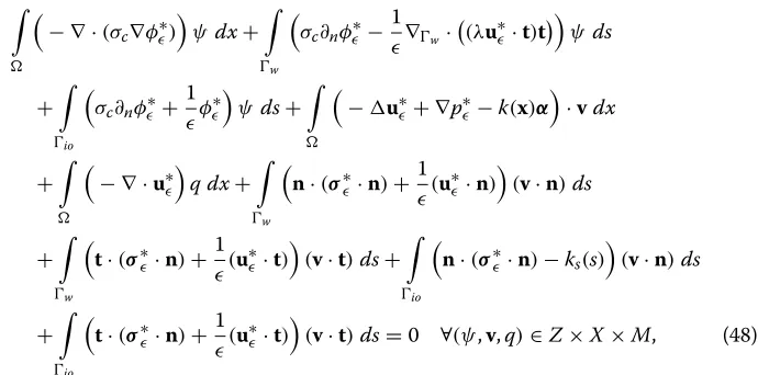
uwall= 0

μ (−∇φ)=λE, (5)

whereEdenotes the applied electric field, and a new parameterλ = 0/μhas been

introduced. Here, is the permitivity (or dielectric constant) of the fluid medium. A detailed derivation of this approximation can be found in a standard reference [19]. The validity of this approximation has been verified for several examples through both experiments and numerical simulations [10].

The associated slip model of EOF can thus be written as:

−∇ ·(σc∇φ)=0 in, (6a)

−μu+ ∇p=0 in, (6b)

∇ ·u=0 in, (6c)

complemented by the boundary conditions,

σc∂nφ=0 onw, (7a)

φ =φio onio, (7b)

u+λ∇φ =0 onw, (7c)

u·t=0 onio, (7d)

problem. This ill-posedness will also be illustrated on numerical examples in Section “Results and discussion”. We decouple one of the velocity components from the potential as follows,

u·t+λ∂tφ =0

u·n+λ∂nφ =0

⇒

u·t+λ∂tφ=0,

u·n=0, (8)

where we have denoted the normal (∇φ·n) and tangential (∇φ·t) derivatives ofφby∂nφ and∂tφ, respectively. This coupling is equivalent to the one given by Eq. (7c). We now proceed to derive the weak formulation for Eq. (6) using the modified coupling given by Eq. (8).

Methods

Variational formulation of the slip BC EOF model Variational formulation of primal problem

We derive here the weak formulation of the equations in Eq. (6) and then combine them to give the coupled problem. The potentialφsatisfies,

−∇ ·(σc∇φ)=0 in, (9a)

φ=φio onio, (9b)

σc∂nφ =0 onw, (9c)

We define C+() as the space of continuous, strictly positive functions on , and assume that the conductivityσc∈C+(). This assumption allows us to simplify the anal-ysis later on and can be easily relaxed. We now introduce the spaces of admissible trial and test functions:

Z=H1(), (10)

Z0= {v∈Z; v=0 onio}, (11)

Zio= {v∈Z; v=φioonio}. (12)

We can use a lift functionφ˜ ∈ Ziosuch thatφ = ϕ+ ˜φwithϕ ∈Z0. In this case, the weak form of the problem is given by:

Givenσc∈C+()andφ˜∈Zio, findϕ∈Z0such that

σc∇ϕ· ∇ψdx= −

σc∇ ˜φ· ∇ψdx, ∀ψ ∈Z0. (13)

We now consider the non-dimensionalized stationary Stokes equations (withμ = 1)

with slip boundaries,

−u+ ∇p=0 in, (14a)

∇ ·u=0 in, (14b)

u·t+λ∂tφ =0 onw, (14c)

u·n=0 onw, (14d)

u·t=0 onio, (14e)

We look for the velocity and pressure fields in the function spaces,

X=H1()2, (15a)

X0=

v∈X; v=0onw, v·t=0 onio , (15b)

M=p∈L2();

p dx=0 . (15c)

Eq. (14c) requires thatφlie in the spaceH2(). Note that if∂is Lipschitz and convex, or C1-continuous, then the elliptic regularity theorem guarantees thatφ ∈H2_(). How-ever, to derive a well-posed adjoint problem for the slip EOF model, we need to enforce the coupling boundary conditions in a weak sense. In fact, if we enforce the condition in a weak sense, the curl theorem shows that it is sufficient to haveφ ∈ Z. Consider the

function spaceH

1 2

0(∂),

H

1 2

0(∂)= {v∈H

1

2(∂)_;v=_{0 onio}}_{. (16)}

We have the following proposition.

Proposition 1.Letbe Lipschitz. Further, let∈Z,λ∈Rand w,g∈H12

0(∂). Define

b(g,w)=g,w

H12,H12

_{and f(w)= −λ ∂t,w}

H−12,H12

_{. Then, the variational problem,}

Find g∈H

1 2

0(∂),such that

b(g,w)=f(w) ∀w∈H12(∂)_{, (17)}

is well-posed, and

g

H12(∂)≤c()|λ| H1(), (18)

where c() is a positive constant that depends only on the domain.

Proof. Since the bilinear formb(g,w)is defined using theH12(∂)_{inner product, it is} bounded and coercive. We can use the curl theorem and a special extension ofwto show the boundedness off(w),

f(w)= −λ∂t,w H−12,H12

₌

∂

−λ∂tw ds.

Consider anH1_{()extension of the functionw, denoted byw˜. From corollary B. 53,} on page 488 in [22], we know that for eachw∈ H12(∂)_{, there exists an extensionw}∗ ∈

H1(), such that,

w∗_H1₍₎≤c()w

H12(∂). (19)

From Proposition 12 in (F.J. Sayas: Weak normal derivatives, normal and tangential traces, and tangential differential operators on Lipschitz boundaries, unpublished), we have,

f(w)= −λ∂t,w H−12,H12

_=λ

Using the fact that the gradient of the curl is the zero vector, and the vector cross product identity, we have,

f(w)= −λ

∇× ∇w∗·k. (20)

We then easily have the following bound on|f(w)|,

|f(w)| ≤ |λ| _H1₍₎w∗_H1₍₎,

≤ |λ| H1₍₎c()w

H12(∂). (21)

Therefore, f

H−12 ≤ c()|λ| H1(), and an application of the Lax-Milgram theorem gives the well-posedness of the variational problem, and the boundg

H12(∂)≤ c()|λ| _H1₍₎.

We can now define the operator:Z→X,

()=(g, 0)on∂, wheregsatisfies Eq. (17), (22a)

()X ≤cg

H12(∂). (22b)

The bounded extension corollary B. 53, on page 488 in [22] implies that there is at least one possible lift for any given. For the purposes of deriving the variational formula-tion, we can pick any admissible lift. It is trivial to show that the operator is linear. Proposition 1 further gives,

()X ≤cg

H12(∂)≤c()|λ| H1(). (23)

Therefore,is a bounded operator. Using this lift operator, we can writeu=w+(φ)= w+(ϕ)+(φ)˜ , wherew∈X0, and write a weak form for Eq. (14),

Givenφ∈Z, find(w,p)∈X0×Msuch that,

∇w· ∇v−p∇ ·v−q∇ ·wdx

= −

∇(φ)· ∇v−q∇ ·(φ)dx ∀(v,q)∈X0×M.

(24)

Combining Eq. (13) and Eq. (24) together, we get the coupled variational statement:

Givenσc∈C+()andφ˜∈Zb, find(ϕ,w,p)∈Z0×X0×Msuch that,

σc∇ϕ· ∇ψdx

+

∇[w+(ϕ)]·∇v−p∇ ·v−q∇·[w+(ϕ)]dx

= −

σc∇ ˜φ· ∇ψdx

−

∇(φ)˜ · ∇v−q∇ ·(φ)˜ dx ∀(ψ,v,q)∈Z0×X0×M,

where we emphasize that the integrals involving the lift velocity, which depend on the solutionϕ, will be part of the bilinear form for this coupled problem. We can recast the bilinear form above in more compact notation as,

Givenσc∈C+()andφ˜∈Zb, findU∈Z0×X0×Msuch that,

A(U,V)=F(V) ∀V∈Z0×X0×M, (26)

whereU=(ϕ,w,p)andV=(ψ,v,q).

We have thus incorporated the coupling condition within our bilinear form and can prove that the coupled problem (26) is well-posed. We refer the interested reader to Appendix A and proceed with the derivation of the corresponding adjoint problem.

Adjoint problem

Given the primal weak form Eq. (26), we have the corresponding weak form for the adjoint problem associated with the quantity of interestQ:Z0×X0×M→R

Givenσc∈C+(), findU∗∈Z0×X0×Msuch that ,

A(V,U∗)=Q(V) ∀V∈Z0×X0×M, (27)

whereU∗=(ϕ∗,w∗,p∗)is the adjoint solution andQ(U)is a linear functional that cor-responds to the quantity of interest (QoI). The full weak form for the adjoint problem reads,

σc∇ψ· ∇ϕ

∗_dx+

(∇v· ∇w

∗_{−q∇ ·w}∗_−p∗_{∇ ·v)dx}

+

(∇(ψ)· ∇w

∗_{− ∇ ·(ψ)p}∗_)dx

=Q(V) ∀V=(ψ,v,q)∈Z0×X0×M. (28)

Note that the adjoint Stokes problem solutionw∗ andp∗ are coupled to the adjoint potentialϕ∗ through the lift operator(·) acting on the test functionψ. The adjoint problem (28) is also well-posed, see Corollary 2 in Appendix A.

We recall that applying the forward coupling condition Eq. (14c) in a strong sense required that the forward potentialφ ∈H2_{(). Correspondingly, to obtain a strong form} corresponding to Eq (28), we require that the adjoint velocityw∗ ∈ H2()2and the adjoint pressurep∗∈H1(). We also have the adjoint stress tensor,

σ∗= −p∗I+(∇u∗+(∇u∗)T). (29) Now integrating by parts we obtain,

− ∇ ·(σc∇ϕ∗) ψdx+

∂

σc∂nϕ∗ψ ds

+

−∇ ·σ∗_·v+(ψ)+ ∂

v+(ψ)·(σ∗·n)ds

+

The boundary term in the formulation of the adjoint problem becomes

∂

v+(ψ)·(σ∗·n)ds

=

w

v+(ψ)·(σ∗·n)ds+

io

v+(ψ)·(σ∗·n)ds

=

w

n·v+(ψ)

0

n·(σ∗·n)+t·v+(ψ) t·(σ∗·n)

−λ∂tψ

t·(σ∗·n)

ds

+

io

n·v+(ψ) n·(σ∗·n)+t·v+(ψ)

0

t·(σ∗·n)ds

=

w

∇w·

λt·(σ∗·n)tψ ds+

io

n·v n·(σ∗·n)ds,

(31)

where we have used integration by parts for the tangential derivative term alongw[23],

w

−(λ∂tψ)(t·z)ds=

w

∇w·

λt·ztψ ds, (32)

where∇w·vdenotes the surface divergence of the vectorv. Replacing these terms in the adjoint formulation and setting,

Q(U)=

k(x)u·αdx+

io

ks(s)u·nds. (33)

We can write Eq. (31) as,

ψ− ∇ ·(σc∇ϕ∗)

dx+

w

ψn·(σc∇ϕ∗) + ∇w·

λt·(σ∗·n)tds

−

v+(ψ)·∇ ·σ∗+k(x)α+

io

n·v+(ψ) n·(σ∗·n−ks(s))

ds

−

q∇ ·w∗dx=0 ∀(ψ,v,q)∈Z0×X0×M. (34)

The strong form of the adjoint system then reads:

∇ ·(σc∇ϕ∗)=0 in, (35a)

−w∗+ ∇p∗=kα in, (35b)

w∗=0 in, (35c)

with three boundary conditions onio:

ϕ∗_{=0 onio, (36a)}

w∗·t=0 onio, (36b)

n·(σ∗·n)=ks onio, (36c)

and three boundary conditions onw:

σc∂nϕ∗+ ∇w·

λt·(σ∗·n)t=0 onw, (37a)

We readily observe that the adjoint Stokes problem can be solved first, independently of the adjoint potential problem, but that the latter does depend on the former through the Neumann coupling condition Eq. (37a). We also note that this coupling condition involves the tangential derivatives of the adjoint stress tensor on the boundary.

Ill-posedness of the adjoint problem for the naive formulation

If both the normal and tangential coupling components are considered in the formulation of the primal problem, the corresponding adjoint boundary integrals (see Eq. (31)) would read,

∂

v+(ψ)·(σ∗·n)ds

=

w

v+(ψ)·(σ∗·n)ds+

io

v+(ψ)·(σ∗·n)ds

=

w

n·v+(ψ) n·(σ∗·n)+t·v+(ψ) t·(σ∗·n)

−λ∂tψ

t·(σ∗·n)

ds

+

io

n·v+(ψ) n·(σ∗·n)+t·v+(ψ)

0

t·(σ∗·n)ds

=

w

−λ ∂nψ

n·(σ∗·n)+

w

∇w·

λt·(σ∗·n)tψ ds

+

io

n·v n·(σ∗·n)ds.

The boundary conditions onwfor the strong form of the adjoint system would then read:

n·(σc∇ϕ∗)+ ∇w·

λt·(σ∗·n)t=0 onw, (38a)

n·(σ∗·n)=0 onw, (38b)

w∗=0 onw. (38c)

Thus the adjoint problem for the ill-posed primal problem contains four boundary con-ditions, despite there being only three variables. Therefore, the ill-posed primal problem leads to an adjoint inconsistent formulation, specifically in the boundary terms. Such an adjoint inconsistency can lead to oscillations in the discrete solutions of the adjoint problem [24].

Penalty formulation of the slip BC EOF model Penalty formulation of the primal problem

the primal solution and the adjoint. The penalty method is an easy and robust approach for applying Dirichlet boundary conditions. See [25] and [26] for analysis of the method. As we shall see, the penalty method is a natural method for weak enforcement of the coupling. In addition, the penalty formulation gives us an adjoint that is asymptotically consistent with the one obtained using the lift technique. The variational formulation Eq. (25) with equivalent penalty boundary conditions can be given as:

Givenσc∈C+()andφio∈H 1

2(_io)_{, find}(φ_,u,p)∈_Z×_X×_{Msuch that,}

σc∇φ· ∇ψ dx+ 1

io

φψ ds+

∇u· ∇v−p∇ ·v−q∇ ·udx

+1

w

(u·n) (v·n)ds+ 1

w

(u·t) (v·t)ds+1

io

(u·t) (v·t)ds

+1

w

λ(∂tφ) (v·t)ds= 1

io

φioψ ds ∀(ψ,v,q)∈Z×X×M. (39)

As was done in Eq. (26), we can recast the bilinear form above in more compact notation as,

Givenσc∈C+()andφio∈H 1

2(_io)_{, findU}∈_Z×_X×_{Msuch that,}

A(U,V)=F(V) ∀V∈Z×X×M, (40)

whereU=(φ,u,p)andV=(ψ,v,q). We now verify that the weak form in Eq. (39) is indeed consistent and converges to the BVP Eq. (9) and Eq. (14) in the limit as the penalty parametertends to zero. Integrating Eq. (39) by parts, we obtain,

− ∇ ·(σc∇φ) ψdx+

w

σc∂nφψ ds+

io

σc∂nφ+1(φ−φio) ψ ds +

(−u+ ∇p)·v−q∇ ·u

ds + w

n·(σ·n)+1 (u·n)

(v·n)ds

+

w

t·(σ·n)+ 1

(λ∂tφ)+u·t)

(v·t)ds+

io

(n·(σ·n)) (v·n)ds

+

io

t·(σ·n)+ 1 (u·t)

v·tds=0 ∀(ψ,v,q)∈Z×X×M, (41)

whereσis the stress tensor corresponding to the penalized solution,

The equivalent strong form for finite non-zerois,

−∇ ·(σc∇φ)=0 in, (43a)

−u+ ∇p=0 in, (43b)

∇ ·u=0 in, (43c)

with the boundary conditions onio:

σc∂nφ+ 1

(φ−φio)=0 onio, (44a)

n·(σ·n)=0 onio, (44b)

t·(σ·n)+ 1

(u·t)=0 onio, (44c)

and the boundary conditions onw:

σc∂nφ=0 onw, (45a)

n·(σ·n)+1

(u·n)=0 onw, (45b)

t·(σ·n)+ 1

(λ∂tφ+u·t)=0 onw. (45c)

One can observe that the penalty method replaces the Dirichlet boundary conditions with a Robin condition. However, upon taking the limit →0 one formally recovers the original problems Eq. (9) and Eq. (14).

Adjoint problem associated with the penalty formulation

We now derive the adjoint problem corresponding to the weak form Eq. (39),

Find(φ∗,u∗,p∗)∈Z×X×Msuch that,

σc∇φ∗· ∇ψ dx+ 1

io φ∗

ψds +

1

w

λ∂tψ(u∗·t)ds

+ 1

w

(u∗·n) (v·n)ds+ 1

w

(u∗·t) (v·t)ds+ 1

io

(u∗·t) (v·t)ds

+

(∇u∗· ∇v−p∗∇ ·v−q∇ ·u∗)dx

=

k(x)v·αdx+

∂

ks(s)v·nds ∀(ψ,v,q)∈Z×X×M. (46)

Using integration by parts for the term involving the tangential derivative alongw[23], i.e.

w

λ∂tψ(u∗·t)ds= −

w ∇w·

and upon integrating by parts the higher-order terms and combining integrals with same test functions, one obtains:

− ∇ ·(σc∇φ∗)

ψ dx+

w

σc∂nφ∗− 1∇w·

(λu∗·t)tψ ds

+

io

σc∂nφ∗+1φ∗

ψds+

−u∗+ ∇p∗−k(x)α

·vdx

+

− ∇ ·u∗

q dx+

w

n·(σ∗·n)+1 (u∗·n)

(v·n)ds

+

w

t·(σ∗·n)+1 (u∗·t)

(v·t)ds+

io

n·(σ∗·n)−ks(s)

(v·n)ds

+

io

t·(σ∗·n)+1 (u∗·t)

(v·t)ds=0 ∀(ψ,v,q)∈Z×X×M, (48)

whereσ∗is the penalized adjoint stress tensor. The equivalent strong form for finite non-zerois,

−u∗+ ∇p∗ =k in, (49a)

∇ ·u∗ =0 in, (49b)

∇ ·(σc∇φ∗)=0 in, (49c)

with the three boundary conditions onio:

n·(σ∗·n)=ks(s) onio, (50a)

t·(σ∗·n)+ 1

(u∗·t)=0 onio, (50b)

σc∂nφ∗+ 1φ∗=0 onio, (50c)

and the three boundary conditions onw:

n·(σ∗·n)+1

(u∗·n)=0 onw, (51a)

t·(σ∗·n)+1

(u∗·t)=0 onw, (51b)

σc∂nφ∗− 1∇w·

(λu∗·t)t=0 onw. (51c)

In the next section, we show that above problem is asymptotically consistent with the previous formulation of the adjoint problem, in the sense that we recover the adjoint corresponding to the strong problem, i.e. Eq. (35), Eq. (36), and Eq. (37) astends to zero.

Consistency of the adjoint penalty problem

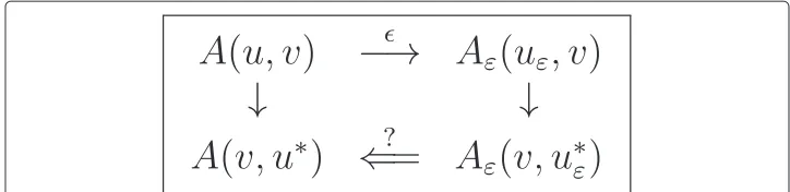
Figure 1 Consistency of the adjoint problems associated with the original and penalty formulations. The question here is whether the adjoint problem obtained from the penalty formulation converges to the adjoint problem derived from the original formulation in the limit when the penalty parametertends to zero.

Recall that the non-penalized adjoint solution (φ∗,u∗) for the problem of interest satisfies the following boundary conditions

φ∗_{=0 on}

io, (52a)

n·(σ∗·n)=k onio, (52b)

u∗·t=0 onio, (52c)

u∗=0 onw, (52d)

σc∂nφ∗+ ∇w·

λt·(σ∗·n)t=0 onw, (52e)

while the penalized adjoint solution (φ∗,u∗) satisfies,

σc∂nφ∗− 1φ∗=0 onio, (53a)

n·(σ∗·n)=k onio, (53b)

t·(σ∗·n)+ 1

(u∗·t)=0 onio, (53c)

t·(σ∗·n)+ 1

(u∗·t)=0 onw, (53d)

n·(σ∗·n)+1

(u∗·n)=0 onw, (53e)

σc∂nφ∗−1∇w·

(λu∗·t)t=0 onw. (53f)

To formally interpret Eq. (53f), we can substitute Eq. (53d) into Eq. (53f) as follows,

t·(σ∗·n)+ 1

(u∗·t)=0⇒ λ

(u∗·t)= −λt·(σ∗·n), σc∂nφ∗= ∇w·

λu∗·t

t

⇒σc∂nφ∗= −∇w·

λt·(σ∗·n)t. (54) We can thus derive the following boundary conditions for the adjoint potential

σc∂nφ∗+ ∇w·

λt·(σ∗·n)t=0 onw, (55a)

φ∗+ σc∂nφ∗ =0 onio, (55b)

which are the same as those for the non-penalized adjoint in the limit→0. Eq. 53d cor-responds to a penalty representation of the tangential boundary flux. Further discussion of this representation is presented in [27]. We thus see that the penalized formulation

of the electroosmotic flow problem is adjoint consistent in the limit as → 0, and

be easily computed by taking the transpose of the stiffness matrix associated with the forward problem.

Results and discussion

We now consider the application of the new EOF formulation on specific microfluidic examples. First, we simulate a flow in a straight microchannel driven purely by electroos-mosis. The objective here is to highlight the convergence and stability properties of the adjoint solution. We then showcase an adjoint-based adaptive strategy for mesh refine-ment on a T-shaped microchannel flow and adjoint-based parameter sensitivity analyses. We discuss the improvement of the convergence rates with respect to quantities of interest and their sensitivities when using adjoint-based techniques. Simulations are per-formed using the adjoint capabilities added to thelibMeshFinite Element library [28]. For both applications, second-order Lagrange elements are employed for the potential and velocity approximations. Linear Lagrange elements are selected to approximate the pressure field in order to satisfy the inf-sup condition. Initial meshes in all the experi-ments dealing with the straight and T-channel domains consist of structured meshes of bi-quadratic quadrilateral elements. Numerical errors to generate the convergence plots are estimated in this work using so-called overkilled reference solutions of the two prob-lems. These are obtained on a uniform mesh of 428,676 degrees of freedom for the straight channel problem and a combined adaptive-uniform mesh with 288,160 degrees of freedom for the T-channel problems. Numerical solutions are calculated using an ILU preconditioned GMRES iterative method for both problems. The linear algebra library

PETSc is accessed throughlibMeshto obtain these solutions. The penalty parameter

was set to the constant value of 10−8for all the numerical experiments.

Electroosmotic flow in a straight channel

Numerical experiments are performed here in the case of an electroosmotic flow in a straight channel. The channel has unit width and the length is five times the width. Since the objective of these simulations is to illustrate the numerical properties of the adjoint solution obtained by using Eq. (39), we set arbitrary values of the model parameters rather than choosing values representative of an actual flow. The fluid viscosityμ, electroos-motic slip parameterκ, and fluid densityρare all taken to be unity. Constant potentials

φi=8 andφo=0 are prescribed at the inletinand outletoutboundaries, respectively. The electric conductivity of the fluid is chosen asσc = 1+x(note that this particular form of the conductivity is chosen for no other reason than better illustrate the properties of the computed adjoint).

The quantity of interest is defined here in terms of the bounded linear functional:

Q(U)=

u·αdx, (56)

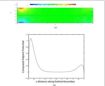
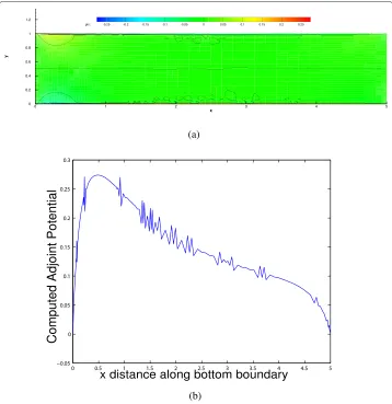
Figure 2 Solutions to the adjoint problem obtained using the penalty formulation Eq. (46).(a)Dual potentialφ∗computed with the penalty formulation.(b)Cutline of computed dual potentialφ∗along the bottom boundary.

solutions with successive mesh refinements, it was numerically verified that the adjoint potential and velocities were all inH1_().

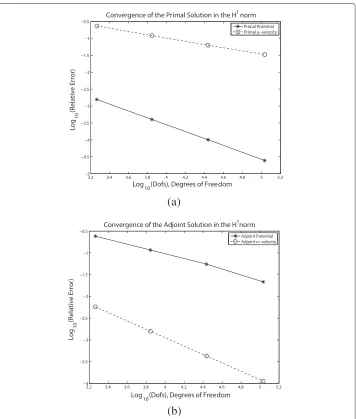
We also studied the convergence rates for the approximate primal and adjoint poten-tial andx-component of the velocity. Recall that the potential and velocity fields are both approximated using second-order Lagrange elements so that one would expect first-order

convergence rates with respect to the number of degrees of freedom in theH1 norm.

However, one can observe in Figure 3 that the primal velocity and the adjoint potential converge at a slower than optimal rate while the primal potential and adjoint velocity converge at the optimal rate. This is due to the tangential ‘slip’ coupling given by Eq. (8) for the forward problem and the Neumann conditions Eq. (55a) for the adjoint prob-lem. Essentially, we can say that the forward Stokes problem and the adjoint potential problem have non-accurate data, leading to higher errors in the computation of their solutions.

Figure 3 Convergence plot for the relative errors in the numerical primal and adjoint potentials and

x-component of the primal and adjoint velocity with respect to theH1()norm.Note the slower rate of convergence for the velocity in the forward problem and the potential in the dual problem.

presence of closed contour lines along the top and bottom wall boundaries. This result is confirmed in Figure 4(b), which shows the solutionφ∗along the top boundary. For uni-form meshes, the instabilities manifest not as oscillations, but a blow-up of the adjoint potential solution in theH1()norm.

Electroosmotic flow in a T-channel

Figure 4 The solutions to the adjoint problems obtained using an ill-posed penalty formulation.(a) Dual potentialφ∗computed with the ill-posed formulation.(b)Cutline of computed dual potentialφ∗along bottom boundary.

is to use adaptive finite element methods to help restore the optimal convergence prop-erties of such singular problems [29]. Likewise, adaptive methods can also improve the convergence behavior of the adjoint solution and potentially restore the optimal rates that one may expect when estimating linear QoIs.

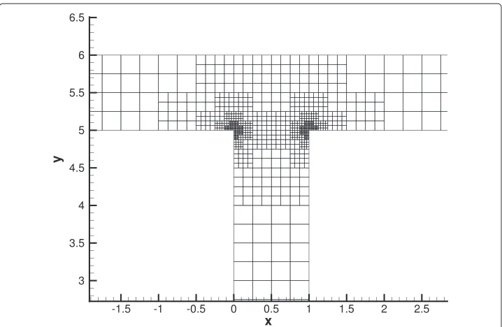
We consider below a T-channel geometry. The two upper ends of the T-channel,i,l andi,r, correspond to the left and right inlets, respectively, at which a high potential

φi is prescribed, while the bottom end of the channelo, the flow outlet, is set to the ground potentialφo = 0. The flow is assumed here to be purely electrically driven, in which case Dirichlet pressure boundary conditionsp= 0 are considered at the inlet and outlet boundaries. The flow parameters used for the numerical experiments are provided in Table 1.

In the numerical experiments below, we consider the following quantity of interest:

Q(U)=

o

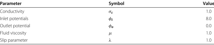
Table 1 Values of the input parameters in the case of the T-channel flow

Parameter Symbol Value

Conductivity _σc 1.0

Inlet potentials φi 8.0

Outlet potential φo 0.0

Fluid viscosity μ 1.0

Slip parameter _λ 1.0

We also estimate the sensitivity of the QoI with respect to the parametersφi,φo, and

λ, evaluated in terms of the first derivativesdQ/dφi,dQ/dφoanddQ/dλ. We used ten adaptive refinement steps followed by two uniform refinements (for a total of 288,160 dofs) to calculate the reference values of these quantities. These values are reported in Table 2 and were used as exact values to compute numerical errors.

The adaptive strategy for mesh refinement with respect to the QoI is described in

Algo-rithm 1, which has been implemented inlibMesh. We show in Figure 5 the horizontal

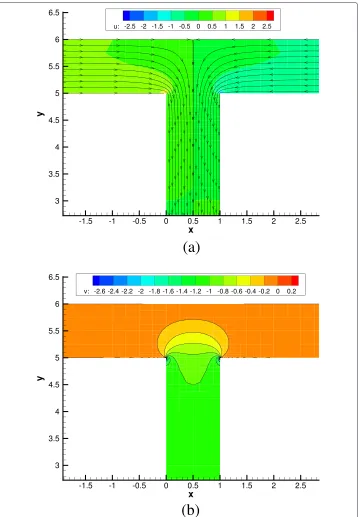
and vertical components of the primal velocityu. We note that the vertical component of the velocity, shown in Figure 5(b), is close to zero near the inlets, but then undergoes a stiff acceleration around the corners. Likewise, we observe in Figure 5(a) the rapid decelera-tion of the horizontal velocity near the corners. This clearly induces a singular behavior of the solution at the two corners. Note also that the solution is symmetric about the cen-terline of the vertical channel, as expected, given that the inlet potentials at stationsi,r andi,lare equal.

Algorithm 1Compute the finite element solution to Eq. (39) that either reaches a pre-scribed mesh sizehminor is obtained after a given number of adaptive stepsnmaxusing an adaptive meshing strategy based on the dual approach with respect to the QoI Eq. (57).

1: Start step counternstep

2: Compute the finite element solutionuhto the problem using a uniform meshMstart

of resolutionhelem=hstart

3: Compute an a posteriori error indicatore˜hfor the QoI based on the adjoint residual error indicator (see [27]) and flag elements to be refined

4: ifhelem ≤hminORnstep>nmaxthen

5: Go to step 11

6: else

7: Refine the top 30 percent of the flagged elements to obtain an adaptive mesh

Madaptive

8: Incrementnstepby 1

9: Repeat steps 2, 3, and 4 using the adapted meshMadaptive

10: end if

11: Postprocess results.

Table 2 Estimated reference values of QoI and of its sensitivity toφi,φo, andκ

Q(U) dQ/dφo dQ/dφi dQ/dλ

Figure 5 Contour plot of the primal solution obtained using the penalty formulation.The singularities are clearly visible in the vicinity of the corners. The solution is smooth away from the corners.(a)

x-componentu1of velocityu.(b)y-componentu2of velocityu.

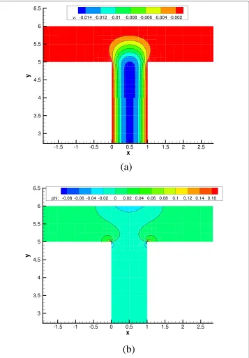
Figure 6 Contour plot of they-component of the adjoint velocityu∗and of the adjoint potentialφ∗.

(a)y-componentu∗₂of adjoint velocityu∗. It is mainly different from zero inside the vertical channel indicating that the primal solution needs to be accurate in that region.(b)Adjoint potential_φ∗. Note that_φ∗ almost vanishes everywhere except at the corners and along the middle section of the top wall.

potential is of course singular at the corners due to the geometrical discontinuity and to the fact that the coupling boundary condition, although almost zero everywhere along the boundaries, becomes non-zero near the corners, since∇w·

Figure 7 Adaptive mesh obtained using adjoint-based error estimates.Note that the elements get refined almost exclusively near the corners due to the singularities in the primal velocity and adjoint potential.

We also used an adjoint method to compute parameter sensitivities for the given QoI to the parameters φi, φo, and λ. The advantage of using an adjoint method for sen-sitivity analysis is that the sensen-sitivity to all three parameters could be found with a single adjoint solve. This is considerably more efficient than using a finite difference or a forward sensitivity method. In addition, we can also combine the adjoint-based mesh refinement and sensitivity analysis for further improvements in the convergence of the sensitivities.

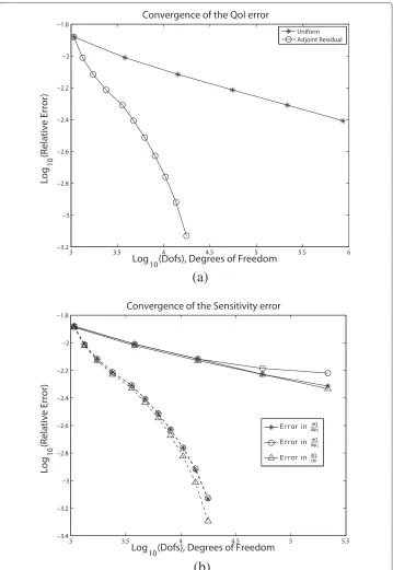
Convergence plots are shown in Figure 8. In particular, the relative error in the quantity of interest estimated using uniform refinement and adjoint-based adaptive refinement is shown in Figure 8(a) against the total number of degrees of freedom (dofs). Relative errors in the estimated sensitivities of the QoI with respect to parameters are displayed in Figure 8(b). We note that the adaptive refinement strategy offers much improved error reduction than uniform refinement for both the estimation of the quantity of interest and its sensitivity derivatives.

In fact, on account of the geometric corner singularities present in the problem, we obtain an inferior convergence rate on using uniform refinement. However, with the adaptive method we obtain a rate of 1.5 (vs dofs) for the QoI, which can be said to be semi-optimal. We had observed earlier that there is a loss of one order in the conver-gence rate for the forward velocity and adjoint potential for the straight channel problem where there are no corner singularities. We recall that with second-order Lagrange Finite Elements this would result in a convergence rate of 1.5 (N1 ×N12) for a linear QoI.

Conclusions

Figure 8 Convergence plots for the approximation of the quantity of interest and its sensitivity to the parametersφi,φo, andλ.(a)Convergence plots for the relative error in QoI Eq. (57) using uniform and adjoint-based refinements.(b)Convergence plots for the relative errors in the sensitivities of the QoI Eq. (57) using uniform and adjoint-based refinements.

the naive formulation”). This leads to instabilities in the computed adjoint, illustrated by numerical experiments in Section “Results and discussion”. A well-posed adjoint problem can be obtained by modifying the slip boundary condition (u+λ∇φ =0), i.e. specifying the normal velocity at the wall independently of the potential (u·n=0,u·t+λ∇φ·t=0). We further proposed a penalty formulation of the forward problem that requires no extra regularity for the potential, and leads to a well-posed, asymptotically consistent adjoint formulation as well. The penalty boundary conditions lead to a weak enforcement of the boundary coupling, allowing us to easily compute the adjoint problem using the adjoint capabilities oflibMesh.

Finally, we presented numerical experiments for a simple straight channel microflow and a more challenging T-channel flow. The convergence results for the straight channel problem indicate that the primal velocity and the adjoint potential converge at sub-optimal rates due to the nature of the coupling between the potential and the velocity. For the T-channel, we presented QoI computation and QoI adjoint sensitivity results for a practical engineering QoI. We observed a loss of convergence order due to the singu-larities in the T-channel geometry, and substantial improvements in the rate on using an adjoint-based adaptive method. However, the fully optimal convergence rate for the QoI could not be achieved, possibly due to the convergence properties of the adjoint potential.

Future work will involve the application of more sophisticated adjoint-based error esti-mators to further improve the convergence properties of the approximate solutions and obtain reliable a posteriori error estimates for complex applications.

Appendix A: Well-posedness of coupled formulation

LetZandXdenote two reflexive Banach spaces. Consider the following abstract linear one-way coupled problem:

Find(φ,u)∈Z×X:

A(φ,ψ)=F(ψ) ∀ψ ∈Z, (58a)

B(u,v)=G(v)−C(φ,v) ∀v∈X, (58b)

where A(·,·), B(·,·), and C(·,·) and continuous bilinear forms, andF(·) and G(·) are continuous linear forms.

If A(·,·) and B(·,·) satisfy the inf-sup conditions on Z ×Z and on X ×X, respec-tively, then the above problem can be solved sequentially: First solve (58a) for φ ∈

Z. Then, since C(φ,·) is a continuous linear form on X, Eq. (58b) can be solved for

u∈X.

The fact that one-way coupled problems (with bounded coupling) are well-posed is probably well known. We now provide an extension of this result for the aggregated bilinear formA(φ,ψ)+B(u,v)+C(φ,v).

Theorem.LetB(·,·),(·,·)denote the aggregated bilinear form:

IfA(·,·)andB(·,·)satisfy the inf–sup conditions, i.e., there exist constantsγA>0 and

γB>0 such that

inf

φ∈Z\{0}_ψ∈supZ\{0}

A(φ,ψ) φZψZ ≥γA

, (59a)

∀ψ ∈Z, ∀φ∈Z, A(φ,ψ)=0=⇒ψ =0, (59b)

inf

u∈X\{0}_v∈sup_X\{0}

B(u,v)

uXvX ≥γB

, (59c)

∀v∈X, ∀u∈X, B(u,v)=0=⇒v=0, (59d)

and ifC(·,·)is a continuous bilinear form, i.e., there is a constantc_C >0 such that

_C(φ,v)≤c_CφZvX ∀φ∈Z,∀v∈X,

thenB(·,·),(·,·)satisfies the inf–sup conditions:

inf

(φ,u)∈Z×X\{0}_(ψ,v)∈supZ×X\{0}

B(φ,u),(ψ,v)

φZ+ uX

ψZ+ vX

≥γ, (60a)

∀(ψ,v)∈Z×X,

∀(φ,u)∈Z×X, B(φ,u),(ψ,v)=0

=⇒(ψ,v)=(0, 0)

,

(60b)

with

1/γ = 1

γA + 1

γB

1+ cC

γA

.

In other words, problem (58) is well-posed. Moreover, the following a priori estimates hold:

φZ≤ 1

γAFZ ∗,

uX ≤ 1

γB

GX∗+

c_C γAFZ

∗

.

Proof.The proof is similar to the Brezzi–Babuška equivalence theorem; see e.g. [22, Proposition 2.36].

We first prove (60a). Using inf-sup stability ofA(·,·)we obtain:

φZ≤ 1

γAψ∈supZ\{0}

A(φ,ψ) ψZ

= 1

γAψ∈supZ\{0}

B(φ,u),(ψ, 0) ψZ

≤ 1

γA(ψ,v)∈supZ×X\{0}

B(φ,u),(ψ,v)

From (58b), inf-sup stability ofB(·,·), and continuity ofC(·,·)we obtain:

uX≤ 1

γBv∈supX\{0} B(u,v)

vX

= _γ1 Bv∈supX\{0}

A(φ, 0)+B(u,v)+C(φ,v)−C(φ,v)

vX

≤ 1

γBv∈supX\{0}

A(φ, 0)+B(u,v)+C(φ,v)

vX +

1

γBv∈supX\{0} C(φ,v)

vX

= _γ1 Bv∈supX\{0}

B(φ,u),(0,v)

vX +

1

γBv∈supX\{0} C(φ,v)

vX

≤ _γ1 Bv∈supX\{0}

B(φ,u),(0,v)

vX +

c_C γBφZ

≤ _γ1

B(ψ,v)∈supZ×X\{0}

B(φ,u),(ψ,v)

ψZ+ vX +

cC γBφZ

≤ _γ1 B

1+ cC

γA

sup

(ψ,v)∈Z×X\{0}

B(φ,u),(ψ,v)

ψZ+ vX .

Finally, summing both contributions,

φZ+ uX≤

1

γA + 1

γB

1+ cC

γA

sup

(ψ,v)∈Z×X\{0}

B(φ,u),(ψ,v)

ψZ+ vX .

To prove (60b), let(ψ,v)∈Z×Xsuch that

0=B(φ,u),(ψ,v) ∀(φ,u)∈Z×X.

Choosing(φ,u)=(0,u), we obtain

0=B(0,u),(ψ,v)=B(u,v) ∀u∈X,

which upon invoking (59d) yieldsv=0. Next, choosing(φ,u)=(φ, 0), we obtain

0=B(φ, 0),(ψ,v)=A(φ,ψ)+C(φ,v)=A(φ,ψ) ∀φ∈Z,

which upon invoking (59b) yieldsφ=0.

Next, we derive the a priori estimates. From inf-sup stability ofA(·,·) and (58a) we obtain:

φZ≤ 1

γAψ∈supZ\{0}

A(φ,ψ) ψZ =

1

γAFZ ∗.

Similarly, using inf-sup stability ofB(·,·), (58b), and continuity ofC(·,·)we obtain:

uX≤ 1

γBv∈supX\{0} B(u,v)

vX

= _γ1 Bv∈supX\{0}

G(v)−C(φ,v)

vX

≤ _γ1 B

GX∗+cCφZ

≤ _γ1 B

GX∗+

c_C γAFZ

∗

Corollary.The weak formulation of the slip-BC EOF model, see (25), is well-posed. We have,

A(ϕ,ψ)=

σc∇ϕ· ∇ψdx, (61)

B((w,p),(v,q))=

∇w· ∇v−p∇ ·v−q∇ ·wdx, (62)

C(ϕ,v)=

∇(ϕ)· ∇v−q∇ ·(ϕ)dx. (63)

Moreover, the following a priori estimates hold:

ϕZ≤

max(σc) min(σc) | ˜φ|H

1₍, (64)

wX+ pM≤ |λ| c()

γB

max(σc) min(σc) | ˜φ|H

1₍₎. (65)

whereγ_Bis the inf-sup constant for the bilinear formB((w,p),(v,q)),λas required by Proposition 1 and c() is as given by Eq. (19).

Proof.It is well known that the variational forms A(ϕ,ψ)andB((w,p),(v,q))satisfy the inf-sup condition [22]. We can use the definition of the operatorin Eq. (22) to easily show thatC(ϕ,v)is bounded,

C(ϕ,v)=

∇(ϕ)· ∇v−q∇ ·(ϕ)dx

≤ |

∇(ϕ)· ∇vdx| + |

q∇ ·(ϕ)dx|

≤ ||(ϕ)H1₍₎|v|_H1₍₎+ q_L2₍₎(ϕ)_H1₍₎

≤ (ϕ)H1₍₎

v_H1₍₎+ q_L2₍₎

≤c()|λ| ϕ_H1₍₎v_H1₍₎+ q_L2₍₎.

(66)

We thus satisfy all the conditions of Theorem 4. We also identfyFas,

F(ψ)= −

σc∇ ˜φ· ∇ψ dx, (67)

whileGis simply the null map. This easily gives the a-priori bounds onϕand(w,p).

Corollary.The weak adjoint problem given by Eq. (28) is well-posed. Moreover, the following a priori estimates hold:

w∗X+ p∗M≤ 1

γBQX

∗ (68)

ϕZ≤

c()|λ|

γBγA QX

Proof. The posedness of the adjoint problem follows directly from the well-posedness of the primal problem (see proposition A.9 in [30]). The bilinear forms for the adjoint variational formulation are,

A(ϕ,ψ)=

σc∇ϕ∗· ∇ψ dx, (70)

B((w∗,p∗),(v,q))=

∇w∗_{· ∇v−q∇ ·w}∗_−p∗_{∇ ·vdx, (71)}

C((w∗,p∗),ψ)=

∇(ψ)· ∇w∗_−p∗_{∇ ·(ψ)dx. (72)}

In an analogous fashion to the one-way coupled formulation of the primal problem (see Eq. (58)), a one-way coupled formulation of the adjoint problem would read,

Find(u,ϕ)∈Z×X:

B(u,v)=Q(v) ∀v∈X, (73a)

A(ϕ,ψ)= −C(u,ψ) ∀ψ ∈Z. (73b)

The inf-sup stability ofB(·,·),A(·,·)and Eq. (73a) and (73b) then easily give the a priori error estimates.

Competing interests

The authors declare that they have no competing interests.

Authors’ contributions

The author’s have presented an adjoint-consistency analysis of the widely used Helmholtz ‘slip’ electroosmotic flow models. It was shown that a direct formulation of such models leads to an ill-posed adjoint problem. A modified formulation is proposed and it is shown that this formulation is well-posed and adjoint-consistent. Numerical

experiments show that the adjoint obtained from the modified formulation can be used for goal-oriented adaptive mesh refinement and adjoint-based sensitivity analysis. All authors read and approved the final manuscript.

Acknowledgements

Vikram Garg is grateful for the support of the Bruton fellowship and the University Continuing fellowship from The University of Texas at Austin. Kris van der Zee is grateful for the support of this work by the 2010 NWO Innovational Research Incentives Scheme (IRIS) Grant 639.031.033. Serge Prudhomme is sponsored by a Discovery Grant from the Natural Sciences and Engineering Research Council of Canada. Serge Prudhomme is also a participant of the KAUST SRI center for Uncertainty Quantification in Computational Science and Engineering.

Author details

1_{Massachusetts Institute of Technology, 77 Massachusetts Avenue, Cambridge, MA 02139, USA.}2_{Ecole Polytechnique de}

Montréal, C.P. 6079, succ. Centre-Ville, Montréal, Canada.3_{The University of Nottingham, Nottingham, UK.}4_{The University}

of Texas at Austin, 1 University Station, C0200 Austin, USA.

Received: 6 February 2014 Accepted: 25 August 2014

References

1. Karniadakis G, Beskok A, Aluru NR (2005) Microflows and Nanoflows: Fundamentals and Simulation. Springer, New York

2. Feynman RP (1960) There’s plenty of room at the bottom. Eng Sci 23(5):22–36

3. Knio OM, Ghanem RG, Matta A, Najm HN, Debusschere B, Le Maˇitre OP (2005) Quantitative Uncertainty Assessment and Numerical Simulation of Micro-Fluid Systems. Technical report, Johns Hopkins University, Baltimore, MD 4. Becker R, Rannacher R (2003) An optimal control approach to a posteriori error estimation in finite element

methods. Acta Numerica 10:1–102

5. Estep D, Carey V, Ginting V, Tavener S, Wildey T (2008) A posteriori error analysis of multiscale operator decomposition methods for multiphysics models. J Phys: Conf Ser 125:012075. IOP Publishing

6. Ionescu-Bujor M, Cacuci DG (2004) A comparative review of sensitivity and uncertainty analysis of large-scale systems. i: Deterministic methods. Nuclear Sci Eng 147(3):189–203

8. Ren L, Sinton D, Li D (2003) Numerical simulation of microfluidic injection processes in crossing microchannels. J Micromech Microeng 13:739

9. MacInnes JM, Du X, Allen RWK (2003) Prediction of electrokinetic and pressure flow in a microchannel T-junction. Phys Fluids 15:1992

10. Hahm J, Balasubramanian A, Beskok A (2007) Flow and species transport control in grooved microchannels using local electrokinetic forces. Phys Fluids 19:013601

11. Craven TJ, Rees JM, Zimmerman WB (2008) On slip velocity boundary conditions for electroosmotic flow near sharp corners. Phys Fluids 20:043603

12. Zimmerman WB, Rees JM, Craven TJ (2006) Rheometry of non-newtonian electrokinetic flow in a microchannel T-junction. Microfluidics Nanofluidics 2(6):481–492

13. Prachittham V, Picasso M, Gijs MAM (2010) Adaptive finite elements with large aspect ratio for mass transport in electroosmosis and pressure-driven microflows. Int J Numerical Methods Fluids 63(9):1005–1030

14. van Brummelen EH, van der Zee KG, Garg VV, Prudhomme S (2012) Flux evaluation in primal and dual boundary-coupled problems. J Appl Mech 79(1):010904. American Society of Mechanical Engineers 15. Estep D, Tavener S, Wildey T (2010) A posteriori error estimation and adaptive mesh refinement for a

multi-discretization operator decomposition approach to fluid-solid heat transfer. J Comput Phys 229:4143–4158 16. Squires TM, Quake SR (2005) Microfluidics: Fluid physics at the nanoliter scale. Rev Modern Phys 77(3):977–1026 17. Whitesides GM (2006) The origins and the future of microfluidics. Nature 442(7101):368–373

18. Chen C, Lin H, Lele S, Santiago J (2005) Convective and absolute electrokinetic instability with conductivity gradients. J Fluid Mech 524:263–303

19. Masliyah JH, Bhattacharjee S (2006) Electrokinetic and Colloid Transport Phenomena. Wiley-Interscience, New York 20. Barz D (2009) Comprehensive model of electrokinetic flow and migration in microchannels with conductivity

gradients. Microfluidics and Nanofluidics 7(2):249–265. Springer

21. Barth WL, Carey GF (2007) On a boundary condition for pressure-driven laminar flow of incompressible fluids. Int J Numerical Methods Fluids 54(11):1313–1325

22. Ern A, Guermond JL (2004) Theory and Practice of Finite Elements, volume 159 of Applied Mathematical Sciences. Springer, New York

23. Delfour M, Zolésio J-P (2001) Shapes and Geometries: Analysis, Differential Calculus, and Optimization. SIAM, New York Vol. 4 of SIAM Series on Advances in Design and Control

24. Hartmann R (2007) Adjoint consistency analysis of discontinuous galerkin discretizations. SIAM J Numer Anal 45(6):2671–2696

25. Babuška I (1973) The finite element method with penalty. Math Comp 27(122):221–228

26. Utku M, Carey GF (1982) Boundary penalty techniques. Comput Methods Appl Mech Eng 30(1):103–118

27. Garg VV (2012) Coupled flow systems, adjoint techniques and uncertainty quantification. PhD Thesis, The University of Texas at Austin

28. Kirk B, Peterson J, Stogner R, Carey G (2006) libMesh: a C++ library for parallel adaptive mesh refinement/coarsening simulations. Eng Comput 22(3):237–254

29. Demkowicz L (2006) Computing with Hp-adaptive Finite Elements: One and Two Dimensional Elliptic and Maxwell Problems. CRC Press, New York

30. Van der Zee K (2009) Goal-adaptive discretization of fluid-structure interaction Dissertation. Delft Institute of Technology, ISBN: 9789079488544 TU Delft institutional repository

doi:10.1186/s40323-014-0015-3

Cite this article as:Garget al.:Adjoint-consistent formulations of slip models for coupled electroosmotic flow systems.Advanced Modeling and Simulation in Engineering Sciences20142:15.

Submit your manuscript to a

journal and benefi t from:

7Convenient online submission 7Rigorous peer review

7Immediate publication on acceptance 7Open access: articles freely available online 7High visibility within the fi eld

7Retaining the copyright to your article